Mesoscopic quantum measurements

Mesoscopic quantum measurements
D.V. Averin
Department of Physics and Astronomy,
SUNY, Stony Brook
A. Di Lorentzo, K. Rabenstein, V.K. Semenov
D. Shepelyanskii, E.V. Sukhorukov

Summary
α 0 + β 1
Example of the trivial wavefunction
reduction:
Basic understanding of quantum
measurements:
the measurement process is
``decoherence with an output’’;
reduction of the wave-function is
a classically trivial act of picking
one random outcome out of several
possibilities.
``Quantum measurement
problem’’: wave function is
typically reduced in an unusual
way, not compatible with the
Schrödinger equation.

Outline
1. Basics
- superconductor and semiconductor single-charge qubits
- QPC as a quantum detector
- ideal quantum detectors: trade-off between information
gain and back-action dephasing in quantum measurements
2. Dynamics of quantum measurements
- linear
- quadratic

R.A. Millikan, Phys. Rev. (Ser. I)
32, 349 (1911).

Quantum dynamics of Josephson
junctions
• Superconductor can be thought of as a BEC of Cooper pairs:
one single-particle state
Ψ =
iϕ
ne
occupied with macroscopic number of particles. The phase φ
and the number of particles n are conjugate quantum variables
(Anderson, 64; Ivanchenko, Zil’berman, 65):
[n,ϕ] =i.
This relation describes dynamics of addition or removal of
particles to/from the condensate.

• If quantum fluctuations of phase φ become large, junction
behavior can be described as a semiclassical dynamics of charge
that leads to controlled transfer of individual Cooper pairs
(D.V. Averin, A.B. Zorin, and K.K. Likharev, 1985):
H
2
= −E
∂ / ∂ϕ
− E cosϕ
=
=
E
C
C
( n − q)
2
2
−
E
J
J
2(
n
n ± 1
+
n ± 1
n
),
E C ≡ (2e)
2
2C
.
2
1.0
(a)
E C
/E J
= 10
(b)
ε 0
/E J
1
0
6
3
1
0.5
−1
0.5
−0.5 −0.3 −0.1 0.1 0.3 0.5
q=V g
C/2e
0.0
0.0 0.2 0.4 0.6 0.8 1.0
q

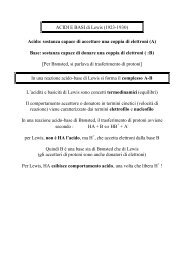
Cooper-pair box as charge qubit
If a small Josephson junction is biased through a capacitor not
resistor, one obtains configuration of a ``Cooper-pair box’’
(M. Buttiker, 1987, H. Pothier et al., 1989) which avoids the problem of
electromagnetic environment.
For E J

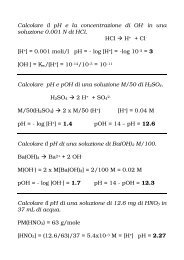
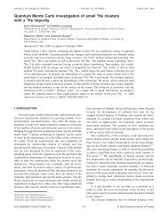
Coherent oscillations in two coupled charge qubits
a
reservoir 2
reservoir 1
probe 2
coupling
island
probe 1
aI 2
( pA)
I 1
(pA)
4
3
13.4 GHz
box 2 box 1
dc gate 2
pulse gate dc gate 1
1µ
m
b E J2, CJ 2 E J1, CJ1
C b2 C b1
V b2 V b1
C m
C g2
C p
C C
p
g1
V g2
V g1
V p
b
c
I 1
(pA)
d
I 2
(pA)
2
5
4
3
2
1
5
4
3
2
1
0
5
4
3
2
1
0
0.0 0.2 0.4 0.6 0.8 1.0
∆t(ns)
Yu. A. Pashkin et al., Nature 421, 823 (2003).
9.1 GHz
0 10 20 30
f(GHz)

Oscillations of probability p j to have a Cooper on the box j=1,2:
2 2
2
1 ⎡
E
1,2 2,1
4
⎤
J
− EJ
+ Em
p1 ,2(1)
= ⎢1
− cos( Ωt)cos(
εt)
−
sin( Ωt)sin(
εt)
⎥,
2 ⎣
4Ωε
⎦
Ω =
2 2 2
( ∆ ) 1/
,
+ E m
2 2 2
( ) 1/
,
δ ∆ = ( E + E ) 2.
ε = δ + E m
= ( EJ
2
− EJ1) 2,
1.0
J1 J 2
Entanglement between the qubits in the process
of oscillations
1
E = 1−
∑ p±
log2 p±
, p±
= 1±
1−
r ,
2
±
E
0.5
r
= 1 2
2
4
Em
2 Em
2 2Em
2
[ 1−
sin ( Ωt)
− sin ( εt)
+ sin ( Ωt)sin
2 ( εt)
+
2
2
2 2
2 Ω
ε
Ω ε
+
∆
2
Ω
2
m
4
E
sin
4
δ
( Ωt)
+
ε
2 2
Em
4
sin
4
( εt)
+
2
m
E
sin(2Ωt)sin(2εt
2Ωε
0.0
)]
0.0 5.0 10.0
t∆/2π
1/ 2
.

Quantum-dot qubits
J.M. Elzerman et al., PRB 767, 161308 (2003).

Quantum antidot qubits
G j
- control gates
Ω- inter-QAD tunnel
amplitude
ε - quasiparticle
"localization"
energy
• Information encoded in the position of a
quasiparticle in the system of two antidots.
• Adiabatic level-crossing dynamics can be used to
transfer quasiparticles between the antidots.
• Conditions of operation: T

Fractional Charge of Laughlin Quasiparticles
V.J. Goldman and B. Su, 1995

Invariance of the quasiparticle charge
V.J. Goldman et al., PRB 64, 085319 (01).

Antidot transport of the FQHE quasiparticles
Antidot ``molecule’’ demonstrates coherent quasiparticle
transport in the double-antidot system
I.J.Maasilta and V.J. Goldman, PRL 84, 1776 (00).

Quantum point contacts (QPC)
M. Field et al., PRL 70, 1311 (1993).
E. Buks et al., Nature 391, 871 (1999).

Mesoscopic quantum measurements II
D.V. Averin
Department of Physics and Astronomy,
SUNY, Stony Brook
A. Di Lorentzo, K. Rabenstein, V.K. Semenov
D. Shepelyanskii, E.V. Sukhorukov

Summary
α 0 + β 1
Example of the trivial wavefunction
reduction:
Basic understanding of quantum
measurements:
the measurement process is
``decoherence with an output’’;
reduction of the wave-function is
a classically trivial act of picking
one random outcome out of several
possibilities.
``Quantum measurement
problem’’: wave function is
typically reduced in an unusual
way, not compatible with the
Schrödinger equation.

Outline
1. Basics
- superconductor and semiconductor single-charge qubits
- QPC as a quantum detector
- ideal quantum detectors: trade-off between information
gain and back-action dephasing in quantum measurements
2. Dynamics of quantum measurements
- linear
- quadratic

Counting statistics in mesoscopic electron transport
(a)
j
I
V
(b)
ε
I
U (x) j
ε+eV
Average current:
Current noise:
∑
I = ( eV / 2πh)
.
k
D k
SI
( 0) = ( eV / 2 πh
) ∑ Dk
(1 − Dk
).
k
Full counting statistics:
(one mode)
P
( N )
n
= C
n
N
D
n
(1 − D)
N −n
,
N = ( eV
L.S. Levitov and G.B. Lesovik, 1993
/ 2πh)
t.

Counting statistics and detector properties of a QPC
( α 0
Detector-induced ``back-action’’
dephasing of the qubit
→ α 0
+ β 1 ) ⊗ in
→
⊗ ( t0 R + r0
L ) + β 1 ⊗ ( t1
R + r1
L
)
( qubit)
ρ out Tr{
R,
L}
ρout
ρin → ρ out
( qubit)
∗ ∗ ∗ ∗
12
( 0 1 0 r1
= ρ = α β → α β t t + r ) ≤ α β
Finally, summing scattering processes of different electrons we
obtain back-action dephasing rate by the QPC detector at T=0:
∗
Γ
d
= −( eV 2πh)ln
| t1 t0
+ r1
r0
∗
∗
| .
The dephasing rate at finite temperature:
[
−1
Γ = ∫ dε
2πh)ln det(1 − f ( ε)
+ f ( ε)
S 0 S )].
d
( 1

Information acquisition rate is determined by distinguishability
of the distributions P j (n) of the transferred charge in different
qubit states:
W
⎛
1/ 2
(1/ )ln [ 0(
) 1(
)] ,
⎟ ⎞
= − t ⎜
∑ P n P n
⎝ n
⎠
The usual counting statistics result for the QPC gives
and
W
∑
n
1/ 2
( )
N
D D R R ,
[ P 0(
n)
P1
( n)]
= 0 1 + 0 1
)ln( ) = − eV 2πh
D D + R R ≤ Γ .
( 0 1 0 1 d
We see that the QPC is an ideal quantum detector with W=Γ d’ if
no information is contained in the phases of the scattering
amplitudes:
φ0 = φ1,
φ j = arg( t j / rj
).
D.V.A. and E.V. Sukhorukov, 2005

An electronic Mach-Zehnder interferometer
Y. Ji et al., Nature 422, 415 (2003).

Phase information can be utilized for measurement if the QPC is
included in the electronic Mach-Zender interferometer:
V
j
r j r’
j
χ
’
t j
t j
S
m
⎛
⎜
i
⎜
⎝
−iχ
Rm
, Dm
e
=
−iχ
Dm
, i Rm
e
⎞
⎟ ⎟ ⎠
The QPC can always be turned into an ideal detector by adjusting
the scattering matrix S m of the second QPC of the interferometer.
If all measurement information is in the phases of the scattering
amplitudes:
φ = φ −φ
≠ , D = ,
this happens if
0 1 0 0 D1
χ = ( φ −φ1) / 2, D m = Rm
0 =
1/ 2.

Conditional qubit evolution
Since transmission and reflection of an electron are classical
alternatives, evolution of the qubit density matrix can be
conditioned on the particular outcome of scattering (following
``quantum-trajectories’’ approach in quantum optics; or A.N. Korotkov, 1999,
in solid-state context). Depending on whether electron is transmitted
or reflected,
| α |
or
2
| α |
2
0
0
0
D0
| α | 0
→
2
[| α | D + | β |
0
Important points:
R0
| α | 0
→
2
[| α | R + | β |
0
2
2
0
D
1
0
]
1/ 2
]
,
1/ 2
• the qubit does not decohere;
0
2
2
R
1
,
αβ
*
αβ
*
0
0
1
1
*
0t1
t αβ 0
→
2
[| α | D + | β |
r
→
[| α |
• probabilities to be in the states 0 and 1 change.
0
2
0
*
1
r
R
0
*
αβ
*
2
0
+ | β |
2
1
D
1
1
R
1
]
1/ 2
]
1/ 2
,
.

Bell-type relation for mesoscopic tunneling
One can devise a simple sequence of qubit transformations
demonstrating that charge is indeed being transferred between the
qubit states even if the tunneling amplitude is vanishing.
Start with the state σ x =1. After transmission of an electron
ψ
=
D 0 0 + D1
1 [ D0
+ D
The sequence of two pulses, one creating tunneling for a period of
time, and another changing the phase between the states 0,1:
∫
∫
1
]
1/ 2
∆( t)
dt / h = π / 4, ε(
t)
dt / h = 2 tan D1
/ D0
−1
.
−π
/ 2,
returns the qubit to the initial σ x =1 state, i.e. we have a closed cycle
which involves tunneling and transfer of charge at ∆=0. For any
classical charge state, there is a probability p to find the state σ x =-1,
p = min{ D0,
D1}
[ D0
+ D
1
]
1/ 2
.

Ballistic Read-out for Flux Qubits
(flux analog of the QPC detector)
f =
1
∆T
Qubit
SFQ pulses Distributed Josephson Junction Voltmeter
mv
H = H 0 + σ z δU
( x)
+ + U ( x)
2
It is convenient to characterize the qubit-detector interaction by the scattering
parameters t 0 ,t 1 ,r 0 ,r 1 .
2

Quantum dynamics of a single fluxon
A. Wallraff et al., Nature 425, 155 (2003).

Generic model of a mesoscopic detector
Detector dynamics should exhibit macroscopically different trajectories (see,
e.g., J.W. Lee et al., 2005) most of the actual mesoscopic detectors are
based on tunneling.
qubit 1 detector
Detector Hamiltonian
H = ( t[
Mˆ
] ξ + h.
c.)
+ Hex,
|0> |1>
t
where ξ creates excitations in the process of particle
transfer between the detector reservoirs.
∆ 1
( n)
& kl
ρ
1 2 2 ( n)
* ( n−1)
* ( n+
1
)( )
)
+ + Γ−
tk
+ tl
ρkl
+ Γ+
tktl
ρij
+ Γ−t
ktl
ρkl
= − ( Γ
2
Γ
+
=
∫
dt ξ(
t)
ξ
+
,
Γ
−
=
∫
+
dt ξ ( t)
ξ .
Ensemble-averaged evolution Conditional evolution
,
ρ&
γ
kl
kl
= −γ
kl
1
= ( Γ
2
ρ
+
kl
+ Γ
− i[
H,
ρ]
−
) t
k
− t
j
kl
,
2
.
ρ
( n)
kl
( τ )
= ρ (0)( Γ
kl
exp{ −(1/
2)( Γ
+
+
/ Γ
−
+ Γ
)
−
n/ 2
)( t
k
I
n
2
(2t
+
t
k
l
t
l
2
Γ
+
Γ
−
) − inϕ
)
kl
}.

Linear quantum measurements
Linear-response theory enables one to develop quantitative
description of the quantum measurement process with an arbitrary
detector provided that it satisfies some general conditions:
• the detector/system coupling is weak so that the detector’s
response is linear;
• the detector is in the stationary state;
• the response is instantaneous.
H
=
H S + H D +
xf
D.V.A., cond-mat/00044364,
cond-mat/0301524.
S.Pilgram and M. Büttiker,
PRL 89, 200401 (2002).
A.A. Clerk, S.M. Girvin, and
A.D.Stone, PRB, (2003).

Information/back-action trade-off in linear
measurements
Dynamics of the measurement process consists of information
acquisition by the detector and back-action dephasing of the
measured system. The trade-off between them has the simplest form
for measurements of the static system with H S =0. If x|j>=x j |j>, we
have for the back-action dephasing:
d
ρ t)
= ρ (0) e , Γ = π ( x − x ) S h .
jj'
( jj'
−Γ
t
Information acquisition by the detector is the process of
distinguishing different levels of the output signal =λx j in the
presence of output noise S q . The signal level (and the corresponding
eigenstates of x) can be distinguished on the time scale given by the
by the measurement time τ m :
2
τ = 8πS
[ λ(
x − x )] , τ Γ = 8( π hλ)
S S ≥ 1 2.
m
q
j
j'
m
d
d
j
j'
2
2
q
f
f
2

FDT analog for linear quantum measurements
h λ ≤ 4π
[ S
f
S
q
−
(Re S
fq
)
2
]
1/ 2
,
where λ is the linear response coefficient of the detector, S f and S q
are the low-frequency spectral densities of the, respectively, backaction
and output noise, ReS fq is the classical part of their crosscorrelator.
As one can see, this inequality characterizes the efficiency of the
trade-off between the information acquisition by the detector and
back-action dephasing of the measured system. The detector that
satisfies this inequality as equality is ``ideal’’ or ``quantumlimited’’.

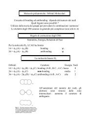
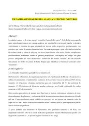
Continuous monitoring of the MQC oscillations
The trade-off between the information acquisition by the detector
and back-action dephasing manifests itself in the directly
measurable quantity in the case of measurement of coherent
quantum oscillations in a qubit.
H = −
∆ σ + σ f +
2
x
z
H
D
Spectral density S o (ω) of the detector output reflects coherent
quantum oscillations of the measured qubit:
S o ( ω)
= S q
+
Γ
d
λ
4π
2
( ω
The height of the oscillation peak in the output spectrum is limited
by the link between the information and dephasing:
2
− ∆
Smax S q ≤ 4.
2
∆
)
2
2
+ Γ
2
d
ω
2
.

12
12
ε=0.7∆
S o
/S q
8
Γ=0.1∆
S o
/S q
8
Γ/∆= 1.5
1.0
4
4
0.7
Ω/∆=1.0 1.5 2.0
0.3
0
0 1 2
ω/∆
0
0.1 0.03
0 1 2
ω/∆
A.N.Korotkov and D.V.A.,
Phys. Rev. B 64, 165310 (2001).

Experimental continuous monitoring of the Rabi
oscillations
M
L L T C T
S V,max
/S 0
1
0.5
(a)
a
b
c
ω R
/ω T
1.1
1
(b)
a
b
c
E.Il’ichev et al.,PRL 91,
097906 (2003).
0
0.96 0.98 1 1.02 1.04
(P/P 0
) 1/2
0.9
0.96 0.98 1 1.02 1.04
(P/P 0
) 1/2

Quadratic measurements
t [ Mˆ
] = t + c Mˆ
+ c
ˆ
2
0 1 2M
,
Example: DC SQUID
Mˆ
1
(1)
z
= λ σ + λ σ
2
(2)
z
t(
Mˆ
)
= t
(1) (2) (1) (2)
0 + δ 1σ
z + δ 2σ
z + λσ z σ z
Purely quadratic measurements, δ j =0.
H 0 = 0
.
Quadratic measurement distinguishes ``parallel’’ from the ``antiparallel’’
qubit state, i,.e., is the measurement of the product operator
of the two qubits σ z
(1)
σ z
(2)
.
The measurement time is
τ
S
I
m
0
a
=
S
= ( Γ
= ( I
0
+
↑↑
/ I
2
a
,
+ Γ
− I
−
)(| t
↑↓
0
|
2
+ | λ |
) / 2 = ( Γ
+
2
),
0
*
*
0
− Γ )( t λ + t λ).
−
t(
Φ)
=
E J
2
(1 −π
Φ
Φ

∑
H0 = −∆ 2 σ x
j
( j)
In this case, quadratic measurements can entangle two non-interacting symmetric
qubits. Indeed, there are three possible measurement outcomes. In the first two,
the qubits are entangled:
I
I
I
I
0
= I
= I
= I
0
0
0
+ I
− I
,
λ
λ
= ( Γ+ − Γ−
)(| t
,
,
ψ ∈
ψ = ↑↑ − ↓↓ ,
ψ
{ ↑↑ + ↓↓ , ↑↓ + ↓↑ },
0
|
2
=
↑↓
+ | λ |
−
2
).
↓↑
,
In the third outcome, the qubits perform coherent qubit oscillations at frequency
that is twice the oscillation frequency of individual qubits.
S
I
( ω)
=
S
0
+
( ω
2
γ =
8I
− 4∆
a
2
2( Γ
∆
)
2
2
γ
+ γ
+ + Γ−
2
ω
) λ
2
2
.
,
W. Mao et al., PRL 93, 056803 (04)

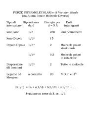
Continuously-measured spectroscopy of two qubits
Non-linear measurements,
δ j ≠0, λ≠0.
(1) (2)
0 −∆
σ z
j
S I
/S 0
t = t0 + 2δS z + λ(2Sz
−1).
2
2 I jγ
j
w ≈ j∆,
SI
( ω)
= S0
+
,
2 2
3 ( ω − j∆)
+ γ j
2 2
γ 1 = ( Γ+
+ Γ−
)(| δ | + | λ | / 2), γ 2 = 2γ
1,
I1
= ( I↑↑
− I↓↓) / 2, I2
= ( I↑↑
+ I↓↓
− 2I↓↑) / 2.
I = ( I↑↑ + I↓↓
+ I↓↑ ) / 3
( j)
H = 2∑ σ x + ( ν 2) σ z .
2
S I
/S 0
12
8
4
0
8
4
ν/∆=0.0
1.0
0.1
0.2
0
0 1 2
W. Mao et al., PRB 71, 085320 (05)
ω/∆
(a)
(b)