The Pantograph Mk-II: A Haptic Instrument - CIM - McGill University
The Pantograph Mk-II: A Haptic Instrument - CIM - McGill University
The Pantograph Mk-II: A Haptic Instrument - CIM - McGill University

Create successful ePaper yourself
Turn your PDF publications into a flip-book with our unique Google optimized e-Paper software.
Proc. IROS 2005, IEEE/RSJ Int. Conf. Intelligent Robots and Systems, pp. 723-728.<br />
the tip and the end effector is equidistant from the actuated<br />
joints. Here, the Jacobian matrix maps disks in the angular<br />
velocity joint space to disks in the tip velocity space. <strong>The</strong>re<br />
are just two such points. <strong>The</strong> other point which has a negative<br />
y is not used. <strong>The</strong> isotropic region is near the edge of the<br />
worskspace but this is an acceptable compromise given that<br />
the main objective is dynamic performance. <strong>The</strong> device, as<br />
dimensioned, has a large region of dynamic near-isotropy<br />
spreading over most of the workspace [13].<br />
y (mm)<br />
40<br />
60<br />
80<br />
3.25<br />
2.55<br />
1.95<br />
1.45<br />
100<br />
1.01<br />
40 20 0 -20 -40 -60<br />
x (mm)<br />
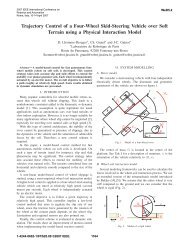
Fig. 5. Condition number of the Jacobian of the <strong>Pantograph</strong> over the<br />
workspace. <strong>The</strong> device is isotropic at the point P iso .<br />
If ‖ · ‖ 2 denotes the largest singular value of a matrix, then<br />
expression:<br />
‖∆X‖ ≤ ‖J‖ 2 ‖[∆θ 1 ∆θ 5 ] ⊤ ‖ (24)<br />
where ∆X = [∆x ∆y] ⊤ is the resolution of the device and<br />
∆θ i the resolution of an encoder. This allows us to plot the<br />
ideal resolution of the device in Fig. 6 for the case where<br />
encoders with 65K CPR are used.<br />
y (mm)<br />
40<br />
60<br />
80<br />
100<br />
9 9<br />
8.6<br />
9<br />
40 20 0 -20 -40 -60<br />
x (mm)<br />
Fig. 6. Resolution of the <strong>Pantograph</strong> in the workspace, measurement unit<br />
is the µm. <strong>The</strong> device is equipped with two√ encoders with 2 16 counts per<br />
revolution, the resolution is ‖∆X‖ = ‖J‖ 2 2<br />
2π<br />
2 16 .<br />
E. Calibration<br />
Since the angles are measured by incremental encoders, the<br />
origin needs to be calibrated at system startup. <strong>The</strong> workspace<br />
of the device is mechanically limited to a rectangular area<br />
which can be used for this purpose. In a first maneuver, point<br />
P 3 is brought by the user to the bottom left corner of the<br />
workspace to roughly calibrate the encoders. <strong>The</strong> user then<br />
proceeds to acquire many calibration points by sliding the end<br />
effector along the four edges (bottom, right, top, left). Points<br />
12<br />
11<br />
10<br />
acquired on the bottom edge all have the same y coordinate,<br />
so on this edge, P i↓<br />
3 = (x i 3, y ↓ ) where y ↓ is the known<br />
common value of the coordinate, and similarly for the other<br />
edges: y ↑ for the top edge, x ← for the left edge, and x → for<br />
the right.<br />
Call the θ1 i and θ5, i the measurements acquired. <strong>The</strong> components<br />
of the direct kinematic function are x 3 and y 3 :<br />
P 3 = [x 3 (θ 1 , θ 5 ) y 3 (θ 1 , θ 5 )] ⊤ . <strong>The</strong> device can be calibrated<br />
by minimizing the error function<br />
E = ∑ N ↓<br />
i=1 [y↓ − y 3 (θ i↓<br />
1 + θ0 1, θ i↓<br />
5 + θ0 5)] 2 +<br />
∑ N→<br />
i=1 [x→ x 3 (θ1 i→ + θ1, 0 θ5 i→ + θ5)] 0 2 +<br />
∑ N↑<br />
i=1 [y↑ − y 3 (θ i↑<br />
1 + θ0 1, θ i↑<br />
5 + θ0 5)] 2 +<br />
∑ N←<br />
i=1 [x← − x 3 (θ1 i← + θ1, 0 θ5 i← + θ5)] 0 2 , (25)<br />
over the zero positions θ1 0 and θ5: 0 min θ 0<br />
1 ,θ5 0 E. This is accomplished<br />
using the Levenberg-Marquardt algorithm [8]. <strong>The</strong><br />
results are satisfying since the two offset angles are found<br />
with an uncertainty of 6-7 counts which can be attributed<br />
to backlash in the joints 2 and 4 as further discussed in<br />
Section IV-B.<br />
IV. RESULTS<br />
<strong>The</strong> importance of the static and dynamic behavior of<br />
haptic devices, accounting for the mechanical structure, transmission<br />
and drive electronics has been well recognized by<br />
device designers [1], [2], [7], [14], [20], [23].<br />
Guidelines for measuring the performance characteristics<br />
of force feedback haptic devices were documented in [12].<br />
Among these guidelines two are particularly important, in<br />
addition to the usual requirement of minimizing interference<br />
with the process being measured. <strong>The</strong> first specifies that<br />
the characteristics must be measured where the device is<br />
in contact with the skin. <strong>The</strong> second recognizes the fact<br />
that a haptic device has a response that depends on the<br />
load. <strong>The</strong>refore, load reflecting the conditions of actual use<br />
must be applied during the measurements. From this view<br />
point, measurement of the system response from the actuator<br />
side and without a load, as it is sometimes done (e.g. [4]),<br />
fails to provide the sought information. A useful actuatorside<br />
technique that quantifies the structural properties of a<br />
device in terms of a “structural deformation ratio” (SRD) was<br />
nevertheless suggested [19]. It was not used here since the<br />
complete system response provides richer information.<br />
A. Experimental System Response<br />
<strong>The</strong> frequency response (from amplifier current command<br />
to acceleration at the tip) was measured with a system<br />
analyzer (DSP Technology Inc., SigLab model 20-22) using<br />
chirp excitation. This technique was used because it is more<br />
precise and more robust to nonlinearities (and more time<br />
consuming) than an ARMAX procedure.<br />
Measurements were performed under three conditions. <strong>The</strong><br />
first corresponded to the unloaded condition. In order to<br />
prevent the device from drifting away during identification, it<br />
was held in place by a loosely taught rubber band. <strong>The</strong> second