Chapter 5 Steady and unsteady diffusion
Chapter 5 Steady and unsteady diffusion
Chapter 5 Steady and unsteady diffusion

Create successful ePaper yourself
Turn your PDF publications into a flip-book with our unique Google optimized e-Paper software.
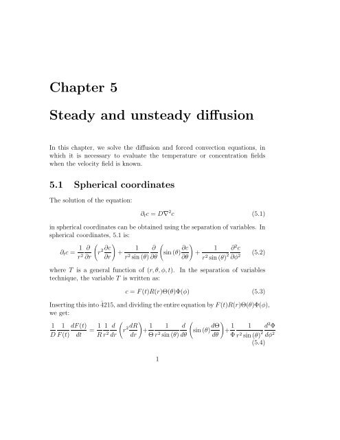
<strong>Chapter</strong> 5<br />
<strong>Steady</strong> <strong>and</strong> <strong>unsteady</strong> <strong>diffusion</strong><br />
In this chapter, we solve the <strong>diffusion</strong> <strong>and</strong> forced convection equations, in<br />
which it is necessary to evaluate the temperature or concentration fields<br />
when the velocity field is known.<br />
5.1 Spherical coordinates<br />
The solution of the equation:<br />
∂ t c = D∇ 2 c (5.1)<br />
in spherical coordinates can be obtained using the separation of variables. In<br />
spherical coordinates, 5.1 is:<br />
∂ t c = 1 ( )<br />
(<br />
∂<br />
r 2∂c 1 ∂<br />
+ sin (θ) ∂c )<br />
1 ∂ 2 c<br />
+<br />
r 2 ∂r ∂r r 2 sin (θ) ∂θ ∂θ r 2 sin (θ) 2 (5.2)<br />
∂φ 2<br />
where T is a general function of (r, θ, φ, t). In the separation of variables<br />
technique, the variable T is written as:<br />
c = F(t)R(r)Θ(θ)Φ(φ) (5.3)<br />
Inserting this into˚4215, <strong>and</strong> dividing the entire equation by F(t)R(r)Θ(θ)Φ(φ),<br />
we get:<br />
1 1 dF(t)<br />
= 1 ( )<br />
1 d<br />
r 2dR + 1 (<br />
1 d<br />
sin (θ) dΘ )<br />
+ 1 1 d 2 Φ<br />
D F(t) dt R r 2 dr dr Θ r 2 sin (θ) dθ dθ Φ r 2 sin (θ) 2 dφ 2<br />
(5.4)<br />
1
2 CHAPTER 5. STEADY AND UNSTEADY DIFFUSION<br />
Note that the partial derivatives have now become total derivatives because<br />
F is only a function of t, <strong>and</strong> R, Θ <strong>and</strong> Φ are functions of only r, θ <strong>and</strong> φ<br />
only. The left side of the equation is only a function of t, while the right side<br />
is only a function of (r, θ, φ). Therefore, each side has to be equation to a<br />
constant, say −λ 2 . The solution for F can be easily obtained:<br />
F(t) = exp (−λ 2 t) (5.5)<br />
Note that it is necessary for the constant −λ 2 to be negative for the solution<br />
to be bounded in the limit t → ∞.<br />
The remainder of the equation 5.4 can now be written as:<br />
[ ( ) 1<br />
sin (θ) 2 d<br />
r 2dR + 1 (<br />
1 d<br />
sin (θ) dΘ ) ]<br />
+ λ 2 r 2<br />
R dr dr Θ sin (θ) dθ dθ<br />
= − 1 d 2 Φ<br />
Φ dφ 2 (5.6)<br />
Here, the left side is only a function of r <strong>and</strong> θ, <strong>and</strong> the right side is only a<br />
function of φ. Therefore, both these have to be equal to a constant, say m 2 .<br />
This can be easily solved for the function Φ(φ):<br />
Φ = A 1 sin (mφ) + A 2 cos (mφ) (5.7)<br />
Note that m has to be an integer, because the physical system obtained<br />
remains the same when φ is increased by an angle 2π.<br />
The rest of equation 5.6 can now be written as:<br />
( )<br />
1 d<br />
r 2dR + λ 2 r 2 = − 1 (<br />
d<br />
sin (θ) dΘ )<br />
R dr dr sin (θ) dθ dθ<br />
+ m2<br />
sin (θ) 2 (5.8)<br />
Here, the right side is only a function of θ, while the left side is only a function<br />
of r. Therefore, both sides can be set equal to a constant, n(n + 1). The<br />
equation for Θ then becomes<br />
− 1 (<br />
d<br />
sin (θ) dΘ )<br />
sin (θ) dθ dθ<br />
+ m2<br />
2<br />
= n(n + 1) (5.9)<br />
sin (θ)<br />
The solutions of the above equation are called ‘associated Legendre functions<br />
of degree n <strong>and</strong> order m’:<br />
Θ(θ) = B 1 Pn m (cos (θ) + B 2Q m n (cos (θ) (5.10)
5.1. SPHERICAL COORDINATES 3<br />
Note that just as m was constrained to be an integer in 5.7 <strong>and</strong>˚4221 because<br />
the solution is required to remain unchanged when φ is increased by 2π, in<br />
the above equation n is also an integer because of the functions with non -<br />
integer values of n become infinite at θ = 0. In addition, there is another<br />
stipulation that n > m, because Θ diverges at θ = 0 for n < m. Further, the<br />
functions Q m n (cos (θ)) also become infinite for θ = π, <strong>and</strong> therefore the only<br />
solution for Θ which is finite for both θ = 0 <strong>and</strong> θ = π is:<br />
Θ = B 1 Pn m (cos (θ)) (5.11)<br />
The above solutions are called ‘Legendre polynomials’, because the series<br />
solution for the Legendre equation 5.11 terminates at a certain order. The<br />
first few polynomials are:<br />
P 0 0 = 1 P 0 1 (x) = x<br />
P 0 2 (x) = 1 2 (3x2 − 1) P 1 1 (x) = − √ 1 − x 2<br />
P 1 2 (x) = −3x√ 1 − x 2 P 2 2 (x) = 3(1 − x2 )<br />
(5.12)<br />
Finally, the function R(r) can be determined by solving the left side of<br />
5.8:<br />
d 2 R<br />
dr + 2 [<br />
]<br />
dR<br />
2 r dr + λ 2 n(n + 1)<br />
− R = 0 (5.13)<br />
r 2<br />
The solutions of this equation are called ‘spherical Bessel functions’, which<br />
are given by:<br />
R(r) = C 1 j n (λr) + C 2 y n (λr) (5.14)<br />
where the functions j n <strong>and</strong> y n are related to Bessel functions:<br />
√<br />
j n (x) = π/2xJ n+<br />
1(x)<br />
√ 2<br />
(5.15)<br />
y n (x) = π/2xY n+<br />
1(x)<br />
2<br />
In case we are considering a system at steady state, where the time derivative<br />
of T is zero (so that λ is zero), the spherical Bessel functions assume relatively<br />
simple forms:<br />
R(r) = C 1 r n + C 2 r −n−1 (5.16)<br />
T:<br />
Having obtained the above solutions, we can derive a general solution for<br />
T = R(r)Θ(θ)Φ(φ)F(t)<br />
∞∑ n−1 ∑<br />
= [C 1n j n (λr) + C 2n y n (λr)]Pn m (cos (θ))<br />
n=0 m=0<br />
×[A 1m sin (mφ) + A 2m cos (mφ)] exp (−λ 2 t)<br />
(5.17)
4 CHAPTER 5. STEADY AND UNSTEADY DIFFUSION<br />
where the functions C 1n , C 2n , A 1m <strong>and</strong> A 2n are to be determined from the<br />
boundary conditions.<br />
The solutions˚4220 <strong>and</strong>˚4224 are eigenfunctions of Sturm - Liouville equations,<br />
<strong>and</strong> therefore the eigenfunctions are complete <strong>and</strong> orthogonal. This<br />
orthogonality can be used to determine the constants C 1n , C 2n , A 1n <strong>and</strong> A 2n<br />
in ˚4230. The orthogonality of the sine <strong>and</strong> cosine functions are expressed as:<br />
⎡<br />
∫ 2π<br />
0 for m ≠<br />
dφ sin (mφ) sin (m ′ m′<br />
φ) = ⎣ π<br />
0<br />
for m = m ′<br />
⎡ 2<br />
∫ 2π<br />
0<br />
∫ 2π<br />
0<br />
dφ cos (mφ)cos (m ′ φ) = ⎣<br />
dφ sin (mφ)cos (m ′ φ) = ⎢<br />
⎣<br />
⎡<br />
0 for m ≠ m′<br />
π<br />
for m = m ′<br />
2<br />
0 for m ≠ n <strong>and</strong> (m + n) even<br />
2m<br />
m 2 − n 2 for m ≠ n <strong>and</strong> (m + n) odd<br />
0 for m = n<br />
(5.18)<br />
Similarly, the Legendre polynomials also satisfy the following orthogonality<br />
constraints in the interval 0 ≤ θ ≤ π:<br />
⎡<br />
∫ π<br />
0 for n ≠ n ′<br />
dθ Pn m (cos (θ))P n m (cos (θ)) = ⎢<br />
′ ⎣ 2 (n + m)!<br />
0<br />
5.1.1 Diffusion from a sphere<br />
2n + 1 (n − m)!<br />
5.1.2 Effective conductivity of a composite<br />
for n = n ′ (5.19)<br />
A composite material of thickness L consists of a matrix of thermal conductivity<br />
K m , embedded with particles of radius R <strong>and</strong> thermal conductivity<br />
K p . A temperature gradient T ′ is applied across the composite in the x 3<br />
direction, as shown in figure 5.1, <strong>and</strong> it is necessary to determine the heat<br />
flux q 3 as a function of the temperature gradient T ′ in the x 3 direction. It is<br />
assumed that the length L is large compared to the thickness of the particles<br />
R, so that the material can be viewed as a continuum with an effective conductivity<br />
which is determined by the conduction of heat through the particles<br />
<strong>and</strong> the matrix,<br />
q 3 = −K eff T ′ (5.20)<br />
It is necessary to determine K eff as a function of the conductivities of the<br />
particles <strong>and</strong> the matrix.
5.1. SPHERICAL COORDINATES 5<br />
T+LT’<br />
x<br />
3<br />
q<br />
3<br />
x<br />
1<br />
x<br />
2<br />
T<br />
Figure 5.1: Effective conductivity of a composite material.<br />
If there were no particles, the temperature gradient in the material would<br />
be uniform, <strong>and</strong> the conductivity would be equal to the conductivity of the<br />
matrix. The presence of the particles causes a disturbance to the temperature<br />
field around a particle, which in turn results in a variation in the flux in the<br />
vicinity of the particle. If the concentration of particles is small, so that<br />
the temperature field around one particle is not influenced by the presence<br />
of other particles, the solution can be obtained by considering the effect of<br />
an isolated particle in an infinite matrix, <strong>and</strong> adding this effect for all the<br />
particles in the matrix.<br />
In order to solve this problem, we first consider the effect of a particle on<br />
the temperature field <strong>and</strong> heat flux in the matrix. The particle is considered<br />
to be located at the origin of the coordinate system, as shown in figure 5.2,<br />
<strong>and</strong> a uniform temperature gradient T ′ is imposed in the x 3 direction. At<br />
steady state, the temperature fields in the particle T p <strong>and</strong> in the matrix T m<br />
satisfy the Laplace equation,<br />
∇ 2 T p = 0<br />
∇ 2 T m = 0 (5.21)<br />
At the interface between the particle <strong>and</strong> the matrix, the boundary conditions<br />
require that the temperature <strong>and</strong> the heat flux are equal,<br />
T p<br />
= T m
6 CHAPTER 5. STEADY AND UNSTEADY DIFFUSION<br />
K p<br />
∂T p<br />
∂r<br />
= K m<br />
∂T m<br />
∂r<br />
(5.22)<br />
Though the temperature field is disturbed by the presence of the particle near<br />
the particle surface, it is expected that the temperature field is unaltered at<br />
a large distance from the particle r → ∞, where it is given by<br />
T = T ′ x 3 = T ′ r cos (θ) (5.23)<br />
The temperature field far from the particle can be expressed in terms of<br />
the Legendre polynomial solutions for the Laplace equation as<br />
T = T ′ rP 0 1 (cos (θ)) (5.24)<br />
Since the temperature field is driven by the constant temperature gradient<br />
imposed at a large distance from the particle, it is expected that the temperature<br />
field near the particle will also be proportional to P1 0 (cos (θ)), since<br />
any solution which contains other Legendre polynomials is orthogonal to<br />
P (0)<br />
1 (cos (θ)). Therefore, the solutions for T p <strong>and</strong> T m have to be of the form<br />
T p<br />
T m<br />
= A p1 rP1 0 (cos (θ) + A p2<br />
r P 0 2 1 (cos (θ))<br />
= A m1 rP1 0 (cos (θ) + A m2<br />
r P 0 2 1 (cos (θ)) (5.25)<br />
The constant A p2 is identically zero because T p is finite at r = 0, while<br />
A m1 = T ′ in order to satisfy the boundary condition in the limit r → ∞.<br />
The constants A p1 <strong>and</strong> A m2 are determined from the boundary conditions at<br />
the surface of the sphers,<br />
3T ′<br />
A p1 =<br />
2 + K R<br />
A m2 = (1 − K R)R 3<br />
(5.26)<br />
2 + K R<br />
The temperature fileds in the particle <strong>and</strong> the matrix are<br />
T p =<br />
3T ′ r<br />
P1 0 (cos (θ)<br />
2 + K R<br />
T m = T ′ rP1 0 (cos (θ) + (1 − K R)R 3 T ′<br />
P 0<br />
(2 + K R )r 2 1 (cos (θ)) (5.27)
5.1. SPHERICAL COORDINATES 7<br />
x 3<br />
2<br />
θ<br />
r<br />
x<br />
x<br />
1<br />
Figure 5.2: Coordinate system for analysing temperature field around the<br />
sphere.<br />
The effective conductivity is determined using an effective equation of the<br />
form<br />
〈j e 3〉 = −K eff T ′ (5.28)<br />
where 〈j3 e 〉 is the heat flux along the direction of the temperature gradient,<br />
which is the direction of the imposed temperature gradient. The average<br />
heat flux can be calculated by taking an average over the entire volume of<br />
the matrix,<br />
∫<br />
〈j e 3〉 = 1 V<br />
= − 1 V<br />
dV j3<br />
e<br />
( ∫ )<br />
matrix dV K m(∇T).e 3 +<br />
∫particles dV K p(∇T).e 3<br />
( ∫<br />
composite dV K(∇T).e 3 +<br />
∫particles dV (K p − K m )(∇T).e 3<br />
)<br />
= − 1 V<br />
= − 1 V<br />
(<br />
K m T ′ + NV particle<br />
V<br />
)<br />
3<br />
(K p − K m ) T ′<br />
2 + K R<br />
(5.29)
8 CHAPTER 5. STEADY AND UNSTEADY DIFFUSION<br />
This gives the effective conductivity<br />
K = K m<br />
(<br />
1 + 3(K )<br />
R − 1)<br />
φ<br />
2 + K R<br />
(5.30)<br />
5.2 <strong>Steady</strong> <strong>diffusion</strong> in an infinite domain<br />
5.2.1 Temperature distribution due to a source of energy<br />
Consider a hot sphere of radius R which is continuously generating Q units<br />
of energy per unit time into the surrounding fluid, whose temperature at a<br />
large distance from the sphere is T ∞ , as shown in figure 5.3. The temperature<br />
field in the fluid surrounding the sphere can be determined from the energy<br />
balance equation at steady state,<br />
∇ 2 T = 0 (5.31)<br />
Since the configuration is spherically symmetric, the conservation equation<br />
5.31 is most convenient to solve in a spherical coordinate system in which the<br />
origin is located at the center of the sphere. The energy balance equation is<br />
then given by<br />
(<br />
1 ∂<br />
r ∂T )<br />
= 0 (5.32)<br />
r 2 ∂r ∂r<br />
The solution for this equation, which satisfies the condition T = T ∞ at a<br />
large distance from the sphere, is<br />
T = A r + T ∞ (5.33)<br />
The constant A has to be determined from the condition that the total heat<br />
flux at the surface of the sphere is Q,<br />
−K dT<br />
(4πR 2 ) = Q (5.34)<br />
dr ∣ r=R<br />
This equation can be solved to obtain A = (Q/4πK), so that the temperature<br />
field is<br />
T =<br />
Q<br />
4πKr + T ∞ (5.35)
5.2. STEADY DIFFUSION IN AN INFINITE DOMAIN 9<br />
x<br />
3<br />
r−−>Infinity<br />
T−−>T inf<br />
R<br />
x<br />
2<br />
x<br />
1<br />
r=R<br />
e<br />
j=(Q/4 π<br />
2<br />
R )<br />
Figure 5.3: Temperature field due to heat generation at the surface of a<br />
sphere.
10 CHAPTER 5. STEADY AND UNSTEADY DIFFUSION<br />
Note that the solution for the temperature, 5.35 does not depend on the<br />
radius of the sphere, but only on the total amount of heat generated per unit<br />
time from the sphere. If the object that generates the heat were some other<br />
irregular object, then the temperature field would depend on the dimensions<br />
of the object. However, if we are sufficiently far from the object, so that the<br />
distance from the object is large compared to the characteristic length of the<br />
object, the object appears as a point source of heat, <strong>and</strong> the observer cannot<br />
discern the detailed shape of the object. In this case, it is expected that the<br />
temperature distribution will not depend on the dimensions of the object,<br />
but only on the total heat generated per unit time. Mathematically, a point<br />
source of energy located at the position x 0 is represented by a delta function,<br />
5.2.2 Dirac delta function<br />
S(x) = Qδ(x − x 0 ) (5.36)<br />
The one-dimensional Dirac delta function, δ(x), is defined as<br />
<strong>and</strong><br />
∫ ∞<br />
δ(x) = 0 for x ≠ 0 (5.37)<br />
∫ ∞<br />
dxδ(x) = 1 (5.38)<br />
−∞<br />
−∞<br />
dxδ(x)g(x) = g(0) (5.39)<br />
It is clear from equation 5.39 that δ(x) has dimensions of inverse of length.<br />
The delta function can be considered the limit of the discontinuous function<br />
(figure 5.4)<br />
f(x) = (1/h) for(−h/2 < x < h/2) (5.40)<br />
in the limit h → 0. In this limit, the width of the function tends to zero,<br />
while the height becomes infinite, in such a way that the area under the<br />
curve remains a constant. It is clear that the function f(x) satisfies all three<br />
conditions, 5.37 to 5.39, in the limit h → 0.<br />
In a similar fashion, the three dimensional Dirac delta function, δ(x 1 , x 2 , x 3 )<br />
is defined by<br />
δ(x 1 , x 2 , x 3 ) = 0 for x 1 ≠ 0; x 2 ≠ 0; x 3 ≠ 0 (5.41)<br />
∫ ∞ ∫ ∞ ∫ ∞<br />
dx 1 dx 2 dx 3 δ(x 1 , x 2 , x 3 ) = 1 (5.42)<br />
−∞<br />
−∞<br />
−∞
5.2. STEADY DIFFUSION IN AN INFINITE DOMAIN 11<br />
f(x)<br />
(1/h)<br />
__ −h __ h<br />
2 2<br />
x<br />
Figure 5.4: Dirac delta function in one dimension.<br />
<strong>and</strong> ∫ ∞ ∫ ∞ ∫ ∞<br />
dx 1 dx 2 dx 3 δ(x 1 , x 2 , x 3 )g(x 1 , x 2 , x 3 ) = g(0, 0, 0) (5.43)<br />
−∞ −∞ −∞<br />
The three dimensional Dirac delta function can be considerd as the limit of<br />
the function<br />
f(x 1 , x 2 , x 3 ) = (1/h 3 ) for(−h/2 < x 1 < h/2)<strong>and</strong>(−h/2 < x 2 < h/2)<strong>and</strong>(−h/2 < x 3 < h/2)<br />
= 0 otherwise (5.44)<br />
when h → 0. It is easy to see that this function satisfies all of the above<br />
properties.<br />
5.2.3 Temperature distribution due to a point source<br />
The Greens function for an infinite domain is defined as the temperature (or<br />
concentration) distribution due to a point source of unit strength.<br />
K∇ 2 G = δ(x − x 0 ) (5.45)<br />
The solution for the Greens function on an infinite domain can be obtained<br />
by first shifting the origin of the coordinate system to the position x 0 , so that
12 CHAPTER 5. STEADY AND UNSTEADY DIFFUSION<br />
the radius vector r = x − x 0 , <strong>and</strong> then solving equation 5.45 in a spherical<br />
coordinate system in this coordinate system. In this new coordinate system,<br />
the configuration is spherically symmetric, <strong>and</strong> so the conservation equation<br />
5.45 is<br />
K 1 ∂<br />
r ∂r r∂G = δ(r) (5.46)<br />
∂r<br />
For r ≠ 0, the right side of equation 5.46 is equal to zero, so the solution for<br />
G (upto an additive constant) is<br />
G = 1<br />
4πKr<br />
(5.47)<br />
where A is a constant to be determined from the condition at the origin.<br />
The condition at the origin is most conveniently determined by integrating<br />
equation 5.46 over a small radius ǫ around the origin,<br />
∫ ǫ<br />
−K (4πr 2 )dr<br />
(− A ) ∫<br />
= 1S(x) = dx ′ δ(x − x ′ )S(x ′ ) (5.48)<br />
r 2<br />
0<br />
The solution for the temperature field is then given by<br />
T(x) = 1 ∫<br />
4πK<br />
dx ′ S(x ′ )<br />
|x − x ′ )<br />
(5.49)<br />
Example<br />
A wire of length 2L immersed in a fluid generates heat at the rate of Q<br />
per unit length of the wire per unit time, as shown in figure 5.5. Determine<br />
the temperature field due to this wire.<br />
A cylindrical coordinate system is used, where the z axis is along the<br />
length of the wire, <strong>and</strong> the origin is at the center of the wire. The wire is<br />
considered to be a line of infinitesimal thickness in the x <strong>and</strong> y directions, so<br />
that the energy source due to the wire per unit length is given by<br />
S(x) = Qδ(x)δ(y) for − L < z < L (5.50)<br />
The temperature field, in terms of this source, is given by<br />
T(x) =<br />
=<br />
∫ ∞<br />
0<br />
∫ ∞<br />
0<br />
∫ ∞ ∫ L<br />
dx ′ dy ′ dz ′ G(x − x ′ , y − y ′ , z − z ′ )S(x ′ , y ′ , z ′ )<br />
0<br />
−L<br />
∫ ∞ ∫ L<br />
dx ′ dy ′<br />
0<br />
−L<br />
dz ′Qδ(x′ )δ(y ′ )<br />
4πK<br />
1<br />
((x − x ′ ) 2 + (y − y ′ ) 2 + (z − z ′ ) 2 ) 1/2
5.2. STEADY DIFFUSION IN AN INFINITE DOMAIN 13<br />
x<br />
3<br />
x<br />
2<br />
x<br />
1<br />
2L<br />
Figure 5.5: Heat generation due to a wire.<br />
∫ L<br />
Q<br />
= dz ′ 1<br />
4πK −L (x 2 + y 2 + (z − z ′ ) 2 ) 1/2<br />
⎛ √<br />
= log ⎝ L + z + ⎞<br />
r 2 + (L + z) 2<br />
√<br />
⎠ (5.51)<br />
−L + z + r 2 + (z − L) 2<br />
The formal solution 5.51 can be more conveniently examined as a function<br />
of r at the center of the wire, z = 0,<br />
( √ )<br />
L + r2 + L<br />
T(x) = log<br />
2<br />
−L + √ (5.52)<br />
r 2 + L 2<br />
In the limit r ≫ L, this solution reduces to<br />
T(x) = 2QL<br />
4πKr<br />
(5.53)<br />
This is the solution for the temperature field due to a point source of energy,<br />
as expected when the distance from the source is large compared to the<br />
characteristic length of the source. In the opposite limit r ≪ L, the solution<br />
for the temperature field reduces to<br />
( )<br />
Q 4L<br />
2<br />
T(x) =<br />
4πK log r 2
14 CHAPTER 5. STEADY AND UNSTEADY DIFFUSION<br />
=<br />
Q<br />
2πK log ( 2L<br />
r<br />
)<br />
(5.54)<br />
We will see, a little later, that this is the temperature field due to an infinite<br />
line source of energy in three dimensions, or a point source in two dimensions.<br />
5.2.4 Greens function for finite domains<br />
The Greens function 5.47 is the temperature field due to a point source of<br />
unit strength in a fluid of infinite extent. Most practical problems involve<br />
finite domains, <strong>and</strong> it is necessary to obtain a Greens function which satisfies<br />
the boundary conditions at the boundaries of the domain. In the case of<br />
planar domains, this Greens function is obtained by using ‘image charges’.<br />
For example, consider a point source located at x s = (L, 0, 0) on a semiinfinite<br />
domain bounded by a surface at x 3 = 0, as shown in figure 5.6,<br />
in which the surface has constant temperature equal to T ∞ . In this case,<br />
the Greens function solution of the type 5.47 does not satisfy the condition<br />
(T − T infty ) = 0 at the surface. However, the boundary condition can be<br />
satisfied if we replace the finite domain by an infinite domain, in which<br />
there is a source of strength +1 at (L, 0, 0), <strong>and</strong> a source of strength −1<br />
at x I (−L, 0, 0), as shown in figure 5.6 (a). It is easily seen that due to<br />
symmetry, (T − T ∞ ) is equal to zero everywhere on the plane x 3 = 0, <strong>and</strong><br />
the Greens function which satisfies the zero temperature condition is called<br />
the Dirichlet Greens function G D ,<br />
G D (x =<br />
1<br />
4πK|x − x s | − 1<br />
4πK|x − x I |<br />
(5.55)<br />
The <strong>diffusion</strong> equation is satisfied in the semi-infinite domain x 3 > 0 (since<br />
the Greens function 5.55 satisfies the <strong>diffusion</strong> equation), <strong>and</strong> the boundary<br />
conditions are identical to the required boundary conditions at x 3 = 0,<br />
therefore, the solution G D is the required solution for the Greens function.<br />
Of course, G D predicts a spurious temperature field in the half plane x 3 < 0,<br />
but this is outside the physial domain.<br />
A similar Greens function can be obtained if the boundary condition at<br />
the surface is a zero normal flux condition, j e 3 = 0, at x 3 = 0, instead of the<br />
zero temperature condition. In this case, the zero flux condition is identically<br />
satisfied by imposing a source of equal strength +1 at x I = (−L, 0, 0), as<br />
shown in figure 5.6 (b). The solution for the Greens function with zero flux
5.2. STEADY DIFFUSION IN AN INFINITE DOMAIN 15<br />
(0,0,L)<br />
+Q<br />
x3 (0,0,L)<br />
+Q<br />
00000000000000<br />
11111111111111<br />
T=0<br />
x<br />
x 1<br />
2<br />
(a)<br />
00000000000000<br />
11111111111111<br />
(0,0,−L)<br />
+Q<br />
(0,0,L)<br />
+Q<br />
x3 (0,0,L)<br />
+Q<br />
00000000000000<br />
11111111111111<br />
j=0<br />
e<br />
3<br />
x<br />
x 1<br />
2<br />
(b)<br />
00000000000000<br />
11111111111111<br />
(0,0,−L)<br />
−Q<br />
Figure 5.6: Greens functions for source near a wall with (a) zero temperature<br />
conditions at the wall <strong>and</strong> (b) zero flux conditions at the wall.
16 CHAPTER 5. STEADY AND UNSTEADY DIFFUSION<br />
condition is called the Neumann Greens function G N ,<br />
G N (x =<br />
1<br />
4πK|x − x s | + 1<br />
4πK|x − x I |<br />
(5.56)<br />
A similar procedure could be used for more complicated geometries. The<br />
Greens function for a source in a corner with zero flux conditions, as shown in<br />
figure 5.7(a), could be obtained by using four sources of equal strength placed<br />
symmetrically in an infinite domain. Similarly, the Greens function for a<br />
source in a corner with zero temperature conditions, as shown in figure 5.7(b),<br />
could be obtained by placing two sources <strong>and</strong> two sinks symmetrically in an<br />
infinite domain. The Greens function for a source in a finite channel, as<br />
shown in figure 5.8, would require an infinite number of sources.<br />
5.2.5 Greens function for a sphere<br />
The Dirichlet Greens function G D for a sphere is the solution for the temperature<br />
field due to a source of unit strength which satisfies the zero temperature<br />
condition at the surface of the sphere. This Greens function can be derived<br />
using spherical coordinates (r, θ, φ). Consider a source of strength 1, which<br />
is located, without loss of generality, at x S = (0, 0, r) in a sphere of radius<br />
1, as shown in figure 5.9. The image, by symmetry has to be located along<br />
the line joining the source point <strong>and</strong> the origin, at x I = (0, 0, r ′ ), but the<br />
strength Q I can, in general, be different from that of the source. The temperature<br />
at a point on the surface, x = (r, θ, φ) in spherical coordinates,<br />
or x = (sin (θ)cos (φ), sin (θ) sin (φ), cos (θ)), due to the source <strong>and</strong> sink, is<br />
given by<br />
T =<br />
=<br />
=<br />
1<br />
4πK|x − x I | + Q<br />
4πK|x − x I |<br />
(<br />
1<br />
1<br />
4πK (sin (θ) 2 cos (φ) 2 + sin (θ) 2 sin (φ) 2 + (cos (θ) − r) 2 1/2<br />
)<br />
Q<br />
+<br />
(sin (θ) 2 cos (φ) 2 + sin (θ) 2 sin (φ) 2 + (cos (θ) − r ′ ) 2 ) 1/2<br />
1<br />
4πK<br />
(<br />
1<br />
(1 + r 2 − 2r cos (θ)) 1/2 + Q<br />
(1 + r ′2 + 2r ′ cos (θ)) 1/2 )<br />
(5.57)<br />
The values of Q <strong>and</strong> r ′ are determined from the boundary condition on the<br />
surface of the sphere, which requires that T = 0 for all values of θ <strong>and</strong> φ.
5.2. STEADY DIFFUSION IN AN INFINITE DOMAIN 17<br />
(0,L ,L )<br />
2 3<br />
+Q<br />
+Q<br />
(0,−L ,L )<br />
2<br />
3<br />
(0,L 2<br />
,L 3<br />
)<br />
+Q<br />
000000000000<br />
111111111111<br />
000000000000000<br />
111111111111111<br />
T=0<br />
(0,−L ,−L )<br />
(0,L ,−L )<br />
2 3 2 3<br />
+Q<br />
+Q<br />
(a)<br />
(0,L ,L )<br />
2 3<br />
+Q<br />
−Q<br />
(0,−L ,L )<br />
3<br />
(0,L 2<br />
,L 3<br />
)<br />
+Q<br />
2<br />
−Q<br />
000000000000<br />
111111111111<br />
e<br />
j =0<br />
3<br />
(0,−L ,−L )<br />
+Q<br />
000000000000000<br />
111111111111111<br />
(0,L ,−L )<br />
2 3 2 3<br />
(b)<br />
Figure 5.7: Greens functions for source near a corner with (a) zero temperature<br />
conditions at the walls <strong>and</strong> (b) zero flux conditions at the walls.
18 CHAPTER 5. STEADY AND UNSTEADY DIFFUSION<br />
−Q<br />
(x ,x ,x +3L)<br />
1<br />
2<br />
3<br />
+Q<br />
(x ,x ,x +3L)<br />
1<br />
2<br />
+Q<br />
(x ,x ,x +2L)<br />
1<br />
2<br />
3<br />
+Q<br />
(x ,x ,x +2L)<br />
1<br />
2<br />
3<br />
−Q<br />
(x ,x ,x +L)<br />
1<br />
2<br />
3<br />
+Q<br />
(x ,x ,x +L)<br />
1<br />
2<br />
3<br />
T=0<br />
00000000000000<br />
11111111111111<br />
+Q<br />
(x ,x ,x )<br />
1<br />
2<br />
3<br />
L<br />
j=0<br />
3<br />
00000000000000<br />
11111111111111<br />
+Q<br />
(x ,x ,x )<br />
1<br />
2<br />
3<br />
L<br />
00000000000000<br />
11111111111111<br />
−Q<br />
(x ,x ,x −L)<br />
1<br />
2<br />
3<br />
00000000000000<br />
11111111111111<br />
+Q<br />
(x ,x ,x −L)<br />
1<br />
2<br />
3<br />
+Q<br />
(x ,x ,x −2L)<br />
1<br />
2<br />
3<br />
+Q<br />
(x ,x ,x −2L)<br />
1<br />
2<br />
3<br />
−Q<br />
(x ,x ,x −3L)<br />
1<br />
2<br />
3<br />
+Q<br />
(x ,x ,x −3L)<br />
1<br />
2<br />
3<br />
(a)<br />
(b)<br />
Figure 5.8: Greens functions for source in a channel of finite width with (a)<br />
zero temperature conditions at the walls <strong>and</strong> (b) zero flux conditions at the<br />
walls.
5.2. STEADY DIFFUSION IN AN INFINITE DOMAIN 19<br />
x 3<br />
r’<br />
r<br />
θ<br />
x 1<br />
1<br />
x 2<br />
Figure 5.9: Greens function for a sphere.<br />
This condition is satisfied only if<br />
Q 2 (1 + r 2 ) = 1 + r ′2<br />
2Q 2 r = 2r ′ (5.58)<br />
From these two conditions, the solution for r ′ <strong>and</strong> Q are<br />
r ′<br />
= r −1<br />
Q = r −1 (5.59)<br />
Thus, the solution for the Greens function is<br />
T =<br />
1<br />
4πK|x − x I | + 1<br />
4πKr|x − x I |<br />
(5.60)<br />
where x I = (0, 0, 1/r).
20 CHAPTER 5. STEADY AND UNSTEADY DIFFUSION<br />
5.2.6 Temperature distribution due to a dipole<br />
Consider a source <strong>and</strong> sink of energy, of equal strength, ±Q of energy per unit<br />
time, located at the positions (0, 0, L) <strong>and</strong> (0, 0, −L), as shown in figure 5.10.<br />
The temperature field due to the combination of source <strong>and</strong> sink is given by<br />
Q<br />
T(x) =<br />
4πK(x 2 + y 2 + (z − L) 2 ) +<br />
−Q<br />
(5.61)<br />
1/2 4πK(x 2 + y 2 + (z + L) 2 ) 1/2<br />
If the distance of the observation point from the origin is sufficiently large,<br />
so that the (x, y, z) ≫ L, the temperature field is given by<br />
T(x) =<br />
Q<br />
4πK<br />
= 2QL<br />
4πK<br />
2Lz<br />
(x 2 + y 2 + z 2 ) 1/2<br />
cos (θ)<br />
r 2<br />
= 2QL<br />
4πK r−2 P 1 (cos (θ)) (5.62)<br />
Thus, the temperature distribution due to the combination of a source <strong>and</strong><br />
a sink, in the limit where the distance between the two reduces to zero, is<br />
identical to the second spherical harmonic solution that was obtained for the<br />
Laplace equation. Similarly, it can be shown that the combination of two<br />
sources <strong>and</strong> two sinks, arranged in such a way that the net dipole moment<br />
is zero, corresponds to the third spherical harmonic solution for the Laplace<br />
equation.<br />
5.2.7 Boundary integral technique<br />
In order to solve the steady temperature equation,<br />
we can use a Greens function<br />
∇ 2 T = −S(x) (5.63)<br />
∇ 2 G = δ(x) (5.64)<br />
which is defined according to the required boundary conditions on the domain,<br />
as follows.<br />
∫<br />
dV ′ ∇.(T(x ′ )∇G(x − x ′ ) − G(x − x ′ )∇ ′ T(x ′ ))<br />
∫<br />
= dV ′ (T(x ′ )∇ ′2 G(x − x ′ ) − G(x − x ′ )∇ ′2 T(x ′ ))<br />
= (5.65)
5.2. STEADY DIFFUSION IN AN INFINITE DOMAIN 21<br />
x<br />
3<br />
x<br />
2L<br />
1<br />
+Q<br />
−Q<br />
x<br />
2<br />
Figure 5.10: Temperature field due to a source <strong>and</strong> a sink.<br />
The left side of the above equation can be written as an integral over the<br />
boundary of the domain using the divergence theorem,<br />
∫<br />
dV ′ ∇.(T(x ′ )∇G(x − x ′ ) − G(x − x ′ )∇ ′ T(x ′ ))<br />
∫<br />
= dS ′ n.(T(x ′ )∇G(x − x ′ ) − G(x − x ′ )∇ ′ T(x ′ )) (5.66)<br />
where n is the boundary of the domain. Therefore, the equation 5.66 reduces<br />
to<br />
∫<br />
T(x) + dV ′ G(x − x ′ )S(x ′ )<br />
∫<br />
= dS ′ n.(T(x ′ )∇G(x − x ′ ) − G(x − x ′ )∇ ′ T(x ′ )) (5.67)<br />
5.2.8 Greens function for the <strong>unsteady</strong> <strong>diffusion</strong> equation
22 CHAPTER 5. STEADY AND UNSTEADY DIFFUSION<br />
5.3 Problems<br />
1. Derive the harmonic expansion for a two dimensional cylindrical coordinate<br />
system with coordinates (r, θ).<br />
(a) Use separtion of variables to solve the equation K∇ 2 T = 0 in<br />
cylindrical co-ordinates.<br />
(b) For a point source, solve the heat equation K∇ 2 T = Qδ(x) in<br />
cylindrical coordinates, to obtain the temperature distribution due<br />
to a point source.<br />
(c) What is the temperature field when two sources are located as<br />
shown in figure 1(a) <strong>and</strong> 1(b), <strong>and</strong> L ≪ r Compare with the<br />
second terms in the cylindrical harmonic expansion.<br />
(d) What is the temperature field when four sources are located as<br />
shown in figures 1(c), <strong>and</strong> (d) Compare with the third terms in<br />
the cylindrical harmonic expansion.<br />
(e) Determine the second <strong>and</strong> third terms in the harmonic expansion<br />
by successively taking gradients of the temperature field due to<br />
the point source.<br />
2. Determine the effective thermal conductivity for a dilute array of infinitely<br />
long circular cylinders along the plane perpendicular to the axis<br />
of the cylinders, when the area fraction of the cylinders is φ. Use the<br />
following steps.<br />
(a) Consider an infinitely long cylinder with conductivity K p in a<br />
matrix of conductivity K m , <strong>and</strong> determine the temperature field<br />
around the cylinder when a uniform gradient T ′ is imposed in the<br />
x direction perpendicular to the axis of the cylinder.<br />
(b) Write the heat flux as the sum of the flux over the matrix <strong>and</strong><br />
the sum over the cylinders. When the array is dilute, write the<br />
integral as the sum over one cylinder, <strong>and</strong> determine the thermal<br />
conductivity.<br />
(c) What is the effective conductivity along the axis of the cylinders<br />
3. A point source of heat of strength Q (in units of heat energy per unit<br />
time) is placed at a distance L from a wall.
5.3. PROBLEMS 23<br />
y<br />
y<br />
−Q +Q<br />
x<br />
2L<br />
+Q<br />
x<br />
2L<br />
−Q<br />
(a)<br />
(b)<br />
−Q<br />
y<br />
+Q<br />
x<br />
+Q<br />
y<br />
−Q<br />
+Q<br />
x<br />
+Q −Q<br />
(c)<br />
(d)<br />
−Q<br />
(a) If the wall is perfectly conducting, so that the flux lines at the wall<br />
are perpendicular to the wall as shown in Figure 1(a), determine<br />
the temperature as a function of position.<br />
(b) If the wall is perfectly insulating, so that the flux lines at the wall<br />
are parallel to the wall as shown in Figure 1(b), determine the<br />
temperature as a function of position.<br />
(c) If the wall is not perfectly conducting, but only a fraction f of the<br />
heat on the wall penetrates it, while a fraction (1 − f) does not<br />
penetrate the wall, determine the temperature field as a function<br />
of position.<br />
4. A heater coil in the form of a ring of radius a in the x−y plane generates<br />
heat Q per unit length of the coil per unit time, as shown in figure 2.<br />
(a) If the heater is placed in an unbounded medium of thermal conductivity<br />
K, write an equation for the temperature as a function<br />
of position in the medium.
24 CHAPTER 5. STEADY AND UNSTEADY DIFFUSION<br />
Q<br />
Q<br />
(a)<br />
(b)<br />
Figure 5.11:<br />
(b) Plot the temperature as a function of position along the symmetry<br />
axis of the heater (z axis in the figure). Simplify the expressions for<br />
the temperature for z ≪ a <strong>and</strong> z ≫ a. What does the expression<br />
for z ≫ a correspond to
5.3. PROBLEMS 25<br />
z<br />
y<br />
x<br />
Figure 5.12: