KNIME User's Manual - ISP
KNIME User's Manual - ISP
KNIME User's Manual - ISP

You also want an ePaper? Increase the reach of your titles
YUMPU automatically turns print PDFs into web optimized ePapers that Google loves.
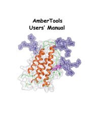
Schrödinger <strong>KNIME</strong> Extensions User <strong>Manual</strong><br />
Schrˆdinger<strong>KNIME</strong><br />
Extensions 1.2<br />
User <strong>Manual</strong><br />
Schrödinger Press
Schrödinger <strong>KNIME</strong> Extensions User <strong>Manual</strong> Copyright © 2009 Schrödinger, LLC.<br />
All rights reserved.<br />
While care has been taken in the preparation of this publication, Schrödinger<br />
assumes no responsibility for errors or omissions, or for damages resulting from<br />
the use of the information contained herein.<br />
Canvas, CombiGlide, ConfGen, Epik, Glide, Impact, Jaguar, Liaison, LigPrep,<br />
Maestro, Phase, Prime, PrimeX, QikProp, QikFit, QikSim, QSite, SiteMap, Strike, and<br />
WaterMap are trademarks of Schrödinger, LLC. Schrödinger and MacroModel are<br />
registered trademarks of Schrödinger, LLC. MCPRO is a trademark of William L.<br />
Jorgensen. Desmond is a trademark of D. E. Shaw Research. Desmond is used with<br />
the permission of D. E. Shaw Research. All rights reserved. This publication may<br />
contain the trademarks of other companies.<br />
Schrödinger software includes software and libraries provided by third parties. For<br />
details of the copyrights, and terms and conditions associated with such included<br />
third party software, see the Legal Notices for Third-Party Software in your product<br />
installation at $SCHRODINGER/docs/html/third_party_legal.html (Linux OS) or<br />
%SCHRODINGER%\docs\html\third_party_legal.html (Windows OS).<br />
This publication may refer to other third party software not included in or with<br />
Schrödinger software ("such other third party software"), and provide links to third<br />
party Web sites ("linked sites"). References to such other third party software or<br />
linked sites do not constitute an endorsement by Schrödinger, LLC. Use of such<br />
other third party software and linked sites may be subject to third party license<br />
agreements and fees. Schrödinger, LLC and its affiliates have no responsibility or<br />
liability, directly or indirectly, for such other third party software and linked sites,<br />
or for damage resulting from the use thereof. Any warranties that we make<br />
regarding Schrödinger products and services do not apply to such other third party<br />
software or linked sites, or to the interaction between, or interoperability of,<br />
Schrödinger products and services and such other third party software.<br />
June 2009
Contents<br />
Document Conventions ...................................................................................................... v<br />
Chapter 1: Introduction ....................................................................................................... 1<br />
1.1 About <strong>KNIME</strong>.............................................................................................................. 1<br />
1.2 About Schrödinger <strong>KNIME</strong> Extensions ................................................................. 1<br />
Chapter 2: <strong>KNIME</strong> Overview .......................................................................................... 3<br />
2.1 The <strong>KNIME</strong> Panel ....................................................................................................... 3<br />
2.2 Nodes........................................................................................................................... 4<br />
2.3 Workflows ................................................................................................................... 5<br />
2.4 Running <strong>KNIME</strong> from the Schrödinger Installation............................................. 6<br />
2.5 Common Tasks .......................................................................................................... 7<br />
Chapter 3: Schrödinger <strong>KNIME</strong> Extensions Tutorial ...................................... 9<br />
3.1 Starting <strong>KNIME</strong> .......................................................................................................... 9<br />
3.2 Creating a New <strong>KNIME</strong> Project.............................................................................. 11<br />
3.3 Adding a Smiles Reader......................................................................................... 13<br />
3.4 Adding the LigPrep and QikProp Nodes............................................................. 15<br />
3.5 Running the Workflow ............................................................................................ 18<br />
3.6 Extracting Properties.............................................................................................. 19<br />
3.7 Writing the Results to Disk in Excel Format ...................................................... 21<br />
3.8 Visualization of the Results.................................................................................. 22<br />
3.8.1 Analyzing the Distribution of Violations of Lipinski’s Rules via a Histogram ..... 22<br />
3.8.2 Plotting the Solvent Accessible Surface Area (SASA) Against the Molecular<br />
Weight.......................................................................................................... 24<br />
3.9 Workflow Samples................................................................................................... 26<br />
Chapter 4: Running Workflows from the Command Line ......................... 27<br />
4.1 The knime Command.............................................................................................. 27<br />
Schrödinger <strong>KNIME</strong> Extensions 1.2 User <strong>Manual</strong><br />
iii
Contents<br />
4.2 Batch Example......................................................................................................... 28<br />
4.3 Modifying Node Settings........................................................................................ 29<br />
4.4 Running Workflows................................................................................................. 32<br />
Getting Help ............................................................................................................................. 33<br />
iv<br />
Schrödinger <strong>KNIME</strong> Extensions 1.2 User <strong>Manual</strong>
Document Conventions<br />
In addition to the use of italics for names of documents, the font conventions that are used in<br />
this document are summarized in the table below.<br />
Font Example Use<br />
Sans serif Project Table Names of GUI features, such as panels, menus,<br />
menu items, buttons, and labels<br />
Monospace $SCHRODINGER/maestro File names, directory names, commands, environment<br />
variables, and screen output<br />
Italic filename Text that the user must replace with a value<br />
Sans serif<br />
uppercase<br />
CTRL+H<br />
Keyboard keys<br />
Links to other locations in the current document or to other PDF documents are colored like<br />
this: Document Conventions.<br />
In descriptions of command syntax, the following UNIX conventions are used: braces { }<br />
enclose a choice of required items, square brackets [ ] enclose optional items, and the bar<br />
symbol | separates items in a list from which one item must be chosen. Lines of command<br />
syntax that wrap should be interpreted as a single command.<br />
File name, path, and environment variable syntax is generally given with the UNIX conventions.<br />
To obtain the Windows conventions, replace the forward slash / with the backslash \ in<br />
path or directory names, and replace the $ at the beginning of an environment variable with a<br />
% at each end. For example, $SCHRODINGER/maestro becomes %SCHRODINGER%\maestro.<br />
In this document, to type text means to type the required text in the specified location, and to<br />
enter text means to type the required text, then press the ENTER key.<br />
References to literature sources are given in square brackets, like this: [10].<br />
Schrödinger <strong>KNIME</strong> Extensions 1.2 User <strong>Manual</strong><br />
v
vi<br />
Schrödinger <strong>KNIME</strong> Extensions 1.2 User <strong>Manual</strong>
Schrödinger <strong>KNIME</strong> Extensions User <strong>Manual</strong><br />
Chapter 1<br />
Chapter 1:<br />
Introduction<br />
1.1 About <strong>KNIME</strong><br />
<strong>KNIME</strong>, the Konstanz Information Miner, is a modular framework (or platform) for graphically<br />
building and executing workflows and data analysis pipelines from predefined components,<br />
called nodes. <strong>KNIME</strong> is developed by Prof. Michael Berthold’s group at the University<br />
of Konstanz in Germany, and can be downloaded free of charge from www.knime.org. Itis<br />
built on the Eclipse Interactive Development Environment (IDE). <strong>KNIME</strong> is implemented in<br />
Java and currently runs on Windows and Linux.<br />
A substantial number of standard data analysis and manipulation tools are distributed with<br />
<strong>KNIME</strong>, which include the following:<br />
• I/O nodes for reading and writing data from files and databases<br />
• Data manipulation nodes for managing the internal data tables that are used to pass information<br />
between components (e.g. filtering rows and columns, partitioning and joining<br />
tables, and so on)<br />
• Charting and plotting tools<br />
• Statistics and data mining tools, such as clustering, neural networks, and decision trees.<br />
Additional features and functionality can be provided as <strong>KNIME</strong> extensions. <strong>KNIME</strong> extensions<br />
are collections of nodes that provide additional capabilities not present in the core<br />
<strong>KNIME</strong> environment. They can very easily be added to an existing <strong>KNIME</strong> installation.<br />
<strong>KNIME</strong> extensions may be licensed differently from the core <strong>KNIME</strong> platform, in particular if<br />
they are provided by third parties or include third party packages. For example, the <strong>KNIME</strong><br />
chemistry extensions provide basic chemistry-related features such as reading and writing of<br />
common data formats and rendering 2D structures via the open-source Chemistry Development<br />
Kit (CDK). Another set of extensions is an interface with R, which a software environment<br />
for statistical computing and graphics. These particular extensions can be downloaded<br />
from the <strong>KNIME</strong> web site.<br />
1.2 About Schrödinger <strong>KNIME</strong> Extensions<br />
Schrödinger has selected <strong>KNIME</strong> as the foundation for its pipelining capabilities. The<br />
Schrödinger <strong>KNIME</strong> extensions provide a large collection of chemistry-related tools that inter-<br />
Schrödinger <strong>KNIME</strong> Extensions 1.2 User <strong>Manual</strong> 1
Chapter 1: Introduction<br />
face with Schrödinger applications and utilities. With the Schrödinger <strong>KNIME</strong> Extensions you<br />
can make use of the full spectrum of Schrödinger applications from within <strong>KNIME</strong> workflows.<br />
These extensions are intended to be well designed and integrated, flexible yet stable and reliable,<br />
and thoroughly tested.<br />
The version of <strong>KNIME</strong> that the Schrödinger extensions are built on is not a proprietary<br />
version, but a freely available core <strong>KNIME</strong> distribution. This means that any other extensions<br />
you develop should work in the absence of the Schrödinger <strong>KNIME</strong> Extensions.<br />
You can of course develop your own extensions that make use of Schrödinger software. To<br />
develop custom nodes you need at least a basic understanding of Java and the <strong>KNIME</strong> API.<br />
Some of the important features that are available through the Schrödinger <strong>KNIME</strong> Extensions<br />
are:<br />
• Ability to assemble, edit and execute workflows using a graphical tool<br />
• Access to most of Schrödinger’s modeling and cheminformatics tools<br />
• Ability to integrate existing command-line tools and scripts<br />
• Interoperability with third party applications<br />
• Web services integration<br />
• Support for distributed and high-throughput computing and compute-intensive modeling<br />
tasks<br />
• Ability to visualize and interact with data at every step of a workflow<br />
• Ability to share workflows<br />
2<br />
Schrödinger <strong>KNIME</strong> Extensions 1.2 User <strong>Manual</strong>
Schrödinger <strong>KNIME</strong> Extensions User <strong>Manual</strong><br />
Chapter 2<br />
Chapter 2:<br />
<strong>KNIME</strong> Overview<br />
This chapter provides an introduction to some of the basic concepts and tasks in <strong>KNIME</strong>. You<br />
can find more information on the <strong>KNIME</strong> web site, at www.knime.org. It also includes information<br />
on running <strong>KNIME</strong> from the Schrödinger distribution.<br />
2.1 The <strong>KNIME</strong> Panel<br />
The main <strong>KNIME</strong> panel, or workbench, contains the following components:<br />
• Menu bar—provides access to a range of tasks.<br />
• Toolbar—Provides shortcuts for common tasks.<br />
• Editor window, or workspace—This is the area in the center where workflows can be<br />
constructed. Each workflow is in a separate tab.<br />
Figure 2.1. The <strong>KNIME</strong> workbench.<br />
Schrödinger <strong>KNIME</strong> Extensions 1.2 User <strong>Manual</strong> 3
Chapter 2: <strong>KNIME</strong> Overview<br />
• Workflow Projects pane—shows all currently defined workflow projects. By default this<br />
pane is at the upper left. This pane has a shortcut (context, right-click) menu that allows<br />
you to perform various tasks on workflows, including creating new workflows, importing<br />
existing workflows, and exporting workflows.<br />
• Favorite Nodes pane—shows nodes in order of last use and in order of frequency of use.<br />
• Node Repository pane—shows all currently available nodes, in a tree view. The nodes are<br />
listed by name, and can be dragged into the workspace. By default this pane is at the<br />
lower left.<br />
• Node Description pane—shows the description of a node.<br />
• Outline pane—shows an outline of the current workflow. By default this pane is at the<br />
lower center.<br />
• Console pane—displays warning and error messages. These messages are also written to<br />
the log file. By default this pane is at the lower right.<br />
2.2 Nodes<br />
The basic unit of a <strong>KNIME</strong> workflow is a node, also called a module. A node corresponds to a<br />
particular task, and is the basic processing unit of a workflow. In the workspace, each node has<br />
the following features:<br />
• A title, at the top<br />
• An icon, in the middle<br />
• Ports for input and output. Each node must have at least one port, and can have multiple<br />
ports of the same type, for different kinds of input or output. The types of ports are:<br />
• Input ports, represented as triangles on the left of the icon, pointing in to the icon.<br />
These ports are for input of data.<br />
• Output ports, represented as triangles on the right of the icon, pointing out from the<br />
icon. These ports are for output of data.<br />
• Model ports, represented as blue squares, on either the right or the left of the icon.<br />
These ports are for input or output of data models.<br />
Each port has a tooltip that displays information about the kind of data that the port<br />
requires or generates.<br />
4<br />
Schrödinger <strong>KNIME</strong> Extensions 1.2 User <strong>Manual</strong>
Chapter 2: <strong>KNIME</strong> Overview<br />
Figure 2.2. Examples of nodes.<br />
• A status display, below the icon. This display usually consists of a set of horizontal “traffic<br />
lights”:<br />
• A red light means that the node is not ready to execute. It might not be fully connected;<br />
it might have incorrect or missing settings; or it might be connected to a<br />
node that is also not ready to execute.<br />
• An amber light means that the node is ready to be executed.<br />
• A green light means that the node has been executed and has sent any output to its<br />
output ports.<br />
When the node is executing, the status display changes to a progress indicator, with a blue<br />
bar.<br />
• A sequence number, below the status display.<br />
• A contextual (right-click) menu, which allows you to configure and execute the node, display<br />
the output views, edit the node, and display data for the ports.<br />
When you select a node, either in the Node Repository or in the workspace, its description is<br />
displayed in the Node Description pane. The description should provide a summary of the<br />
function of the node, a description of its ports, and a description of the available views of the<br />
output.<br />
Warnings and errors are indicated by an icon between the node icon and the status display. The<br />
warning or error message is displayed when you pause the pointer over the warning or error<br />
icon.<br />
2.3 Workflows<br />
A workflow consists of a set of nodes, joined together so that all input and output is defined. To<br />
construct a workflow, drag the desired nodes into the workspace, and connect the ports. The<br />
ports are connected by dragging from the input port on a node to the output port on another<br />
node (or vice versa). Ports that are connected must have compatible data types, which you can<br />
check using the tooltips for the ports. Feedback loops are not permitted: you cannot connect<br />
Schrödinger <strong>KNIME</strong> Extensions 1.2 User <strong>Manual</strong> 5
Chapter 2: <strong>KNIME</strong> Overview<br />
the input of node A to the output of node B if the output of node A is already connected to the<br />
input of node B.<br />
When you have connected all the nodes, you may need to configure some or all of the nodes.<br />
To do so, right-click on the node and choose Configure. The configuration is saved with the<br />
workflow. Re-configuring a node that has been executed resets it: all output is discarded.<br />
To run all of a workflow, choose Execute All from the Node menu, or right-click on the last<br />
node and choose Execute. To execute a workflow up to and including a particular node, rightclick<br />
on the desired node and choose Execute. Workflow execution starts with the first node<br />
that has not already been executed, and continues in sequence through the nodes until the node<br />
that you chose Execute for has been run.<br />
If your <strong>KNIME</strong> installation or <strong>KNIME</strong> extensions is updated, executing any existing workflow<br />
loads and executes the updated nodes. A message is displayed in the Console to notify you of<br />
changes to Schrödinger nodes. You may have to reconfigure the changed nodes to run the<br />
workflow if the node settings have been altered.<br />
2.4 Running <strong>KNIME</strong> from the Schrödinger Installation<br />
When you install <strong>KNIME</strong> and the Schrödinger <strong>KNIME</strong> extensions from the Schrödingerprovided<br />
distribution, they are installed into $SCHRODINGER/knime-vversion, and a script is<br />
installed with which you can run <strong>KNIME</strong>. To do so, use the following command:<br />
$SCHRODINGER/knime [-data directory] [-version] [-help] [-verbose]<br />
The options are described in Table 2.1.<br />
Table 2.1. Interactive options for the knime command.<br />
Option<br />
-data directory<br />
-version<br />
-help<br />
-verbose<br />
Description<br />
Use directory as the <strong>KNIME</strong> workspace. The default is ~/knime_workspace.<br />
Print version number of the Schrödinger extensions and exit<br />
Print information on command line options and exit<br />
Print more information on process and errors.<br />
6<br />
Schrödinger <strong>KNIME</strong> Extensions 1.2 User <strong>Manual</strong>
Chapter 2: <strong>KNIME</strong> Overview<br />
2.5 Common Tasks<br />
To import an archived workflow (zip file):<br />
1. Right click in the Workflow Projects pane, and choose Import <strong>KNIME</strong> workflow from the<br />
shortcut menu.<br />
2. Select Select archive file, and click the corresponding Browse button.<br />
3. Navigate to the desired zip file, and click OK.<br />
4. Click Finish.<br />
To export a workflow to an archive (zip file):<br />
To add a bend in the connection between nodes:<br />
1. Click on theconnection to select it.<br />
2. Pause the cursor over one of the ends of the connection until you see a hand (or on some<br />
systems a double-sided pair of crossed arrows)<br />
3. Drag to create a bend.<br />
To view the output of a node:<br />
1. Right-click on the node.<br />
2. Select Data Outport.<br />
Helpful Hints<br />
• Double click on a tab to enlarge that pane to full screen; double click again to return to<br />
the normal view.<br />
• Drag tabs around to reposition panes. For example, drag the Workflow Project tab next to<br />
the Node Repository tab to have both in the same panel.<br />
• Use the up/down and left/right arrow keys to navigate the nodes in a workflow.<br />
• In tables, right-click on a header to display numbers as bars or in gray scale.<br />
• In tables with 2D structures, drag the row height with the SHIFT key held down to adjust<br />
the height of all rows.<br />
• If you would like to have more control over table width, use the Interactive Table node<br />
(View>Column Width).<br />
• In the molecule Sketcher node, double click on a bond when in “draw bond” mode to<br />
change the bond order.<br />
Schrödinger <strong>KNIME</strong> Extensions 1.2 User <strong>Manual</strong> 7
Chapter 2: <strong>KNIME</strong> Overview<br />
• Cut a node instead of deleting it if you don’t want to see the “Do you really want to delete<br />
...” warning.<br />
8<br />
Schrödinger <strong>KNIME</strong> Extensions 1.2 User <strong>Manual</strong>
Schrödinger <strong>KNIME</strong> Extensions User <strong>Manual</strong><br />
Chapter 3<br />
Chapter 3:<br />
Schrödinger <strong>KNIME</strong> Extensions Tutorial<br />
This chapter provides a tutorial introduction to <strong>KNIME</strong> and the Schrödinger <strong>KNIME</strong> Extensions.<br />
In this tutorial, you will build a workflow that calculates molecular properties for a set of<br />
compounds provided as SMILES strings. The general outline of the workflow is as follows:<br />
• Read a SMILES string from a file<br />
• Carry out 1D to 3D conversion using LigPrep<br />
• Calculate molecular properties using QikProp<br />
• Extract a subset of properties for analysis<br />
• View the molecular properties<br />
3.1 Starting <strong>KNIME</strong><br />
1. Start <strong>KNIME</strong> with the following command:<br />
$SCHRODINGER/knime<br />
While <strong>KNIME</strong> is starting, the following message is displayed in the terminal window:<br />
starting <strong>KNIME</strong> workbench with workspace directory: /home/username/knime_workspace<br />
This message indicates that the workflows will be stored in the directory shown. You can<br />
change the directory by using the -data directory option to the knime command.<br />
A splash screen is also displayed, as shown in Figure 3.1. The splash screen should<br />
include the Schrödinger logo under Installed Extensions. If this logo is missing, the version<br />
of <strong>KNIME</strong> you are running does not have the Schrödinger <strong>KNIME</strong> Extensions, and<br />
you must either add them, or run a version that does.<br />
Figure 3.1. The <strong>KNIME</strong> splash screen.<br />
Schrödinger <strong>KNIME</strong> Extensions 1.2 User <strong>Manual</strong> 9
Chapter 3: Schrödinger <strong>KNIME</strong> Extensions Tutorial<br />
Figure 3.2. The initial <strong>KNIME</strong> window.<br />
If this is the first time you have run <strong>KNIME</strong>, you will see a panel (Figure 3.2) that offers<br />
a choice of downloading additional features or launching <strong>KNIME</strong>. To continue with this<br />
tutorial, click Open <strong>KNIME</strong> workbench to display the <strong>KNIME</strong> workbench.<br />
If you have run <strong>KNIME</strong> previously, the <strong>KNIME</strong> workbench opens directly.<br />
Take some time to examine the layout of the <strong>KNIME</strong> workbench.<br />
At the top there is a menu bar, with a toolbar below it. The View menu allows you to display<br />
various tabs. By default, all are displayed.<br />
On the left side are two tabs, labeled Workflow Projects and Node Repository. The Workflow<br />
Projects tab lists the projects that are available in the current <strong>KNIME</strong> session. The Node<br />
Repository tab lists all the nodes that are available, in a tree structure. At the bottom are two<br />
tabs, Outline and Console. The Outline tab displays an outline of the current workflow. The<br />
Console tab shows error messages or log messages. On the right side is the Node Description<br />
tab, which displays the description of the selected node.<br />
The remaining area is the workspace, where workflows can be constructed, edited, and<br />
executed. The current workflow is highlighted in the Workflow Projects tab.<br />
10<br />
Schrödinger <strong>KNIME</strong> Extensions 1.2 User <strong>Manual</strong>
Chapter 3: Schrödinger <strong>KNIME</strong> Extensions Tutorial<br />
Figure 3.3. The initial <strong>KNIME</strong> workbench.<br />
3.2 Creating a New <strong>KNIME</strong> Project<br />
1. From the File menu, choose New.<br />
The New panel opens. This panel allows you to create a new object using a wizard. In this<br />
case, we want to create a new <strong>KNIME</strong> project.<br />
2. Select New <strong>KNIME</strong> Project in the Wizards list, and click Next.<br />
The next screen is labeled New <strong>KNIME</strong> Project Wizard, and allows you to name the<br />
project.<br />
Schrödinger <strong>KNIME</strong> Extensions 1.2 User <strong>Manual</strong> 11
Chapter 3: Schrödinger <strong>KNIME</strong> Extensions Tutorial<br />
Figure 3.4. The New panel.<br />
3. Enter Molecular Properties in the Name of the project to create text box, and click<br />
Finish.<br />
You should now see a new entry in the Workflow Projects tab and a new tab in the main workspace,<br />
labeled Molecular Properties. To make sure the new project is the active workflow<br />
project, double-click it in the Workflow Projects pane.<br />
Figure 3.5. The New <strong>KNIME</strong> Project Wizard.<br />
12<br />
Schrödinger <strong>KNIME</strong> Extensions 1.2 User <strong>Manual</strong>
Chapter 3: Schrödinger <strong>KNIME</strong> Extensions Tutorial<br />
Figure 3.6. The <strong>KNIME</strong> workbench with the new project.<br />
3.3 Adding a Smiles Reader<br />
The first node (or component) to add to the workflow is a SMILES reader.<br />
1. In the Node Repository, open up the Schrödinger category by clicking on the triangle on<br />
the left side.<br />
2. Open up the Readers/Writers category.<br />
3. Drag the Smiles Reader node into the workspace, and place it on the left.<br />
The node has a title, an icon that represents the node, a set of “traffic lights” that indicates<br />
the status of the node (status indicator), and a node number. The node description is displayed<br />
in the Node Description tab. The icon has a triangle on the right side. This is a<br />
point at which you can connect this node to another node, and represents the output of the<br />
node (the triangle is like an arrowhead pointing out from the node). If you pause the<br />
pointer over this triangle, it displays a brief description of the type of output, in a tooltip.<br />
The node is also added to the Outline tab. As you add nodes, they are added to this tab,<br />
which provides a view of the entire workflow.<br />
Schrödinger <strong>KNIME</strong> Extensions 1.2 User <strong>Manual</strong> 13
Chapter 3: Schrödinger <strong>KNIME</strong> Extensions Tutorial<br />
Figure 3.7. The <strong>KNIME</strong> workbench with the Smiles Reader node, before configuration.<br />
The node initially shows a “red light” because it cannot be run as is, simply because it has<br />
not been configured yet. There is also a warning icon: an exclamation point in a yellow<br />
triangle above the traffic lights. If you pause the pointer over the exclamation point, you<br />
will see that this is a warning message, which tells you that the node needs to be set up.<br />
You might also see a warning message in the Console tab, and also in the terminal window<br />
from which you started <strong>KNIME</strong>. To configure this node, you need to specify the file<br />
it should read.<br />
4. Right click on the Smiles Reader node (anywhere) and choose Configure from the shortcut<br />
menu.<br />
The configuration dialog box for the Smiles Reader node opens.<br />
5. Click Add File(s).<br />
A file dialog box opens that allows you to select a file.<br />
6. Navigate to and select the file $SCHRODINGER/macromodel-vversion/ligprep/<br />
samples/examples/1D_smiles.smi, then click Open.<br />
14<br />
Schrödinger <strong>KNIME</strong> Extensions 1.2 User <strong>Manual</strong>
Chapter 3: Schrödinger <strong>KNIME</strong> Extensions Tutorial<br />
Figure 3.8. The configuration dialog box for the Smiles Reader.<br />
The file is added to the Properties table in the configuration dialog box. This table has<br />
columns for the properties that define how the file is to be used. There is a check box in<br />
the Import all structures column. If you wanted to limit the range of structures imported,<br />
you could deselect the check box, and enter values in the Start and Total columns.<br />
7. Click OK.<br />
The configuration dialog box closes. The warning symbol in the node has gone, and the<br />
“yellow light” is now showing.<br />
3.4 Adding the LigPrep and QikProp Nodes<br />
An alternative way of locating nodes is to use the search text box in the node repository. We<br />
will use this mechanism for subsequent nodes in this tutorial.<br />
1. Type ligprep into the search text box and press ENTER.<br />
The node repository shows all the nodes that match the text entered in the search box. The<br />
search is case-insensitive.<br />
Schrödinger <strong>KNIME</strong> Extensions 1.2 User <strong>Manual</strong> 15
Chapter 3: Schrödinger <strong>KNIME</strong> Extensions Tutorial<br />
Figure 3.9. The <strong>KNIME</strong> workbench with the LigPrep node connected to the Smiles<br />
Reader node.<br />
2. Select the LigPrep node and drag it into the workspace.<br />
3. Connect the Smiles Reader node to the LigPrep node by clicking on the small triangle on<br />
the right side of the Smiles Reader node and dragging the pointer over to the small triangle<br />
on the left of the LigPrep node (see Figure 3.9).<br />
This process connects the output of the Smiles Reader node to the input of the LigPrep<br />
node. When you run the workflow, the structures read by the SMILES reader are passed<br />
on to LigPrep as input.<br />
The default LigPrep settings are appropriate for the calculations carried out in this tutorial<br />
so there is no need to configure the LigPrep node.<br />
If you are curious about what settings are being used, you can open the configuration<br />
panel for the LigPrep node (by right-clicking on the node and selecting Configure) and<br />
examine the settings.<br />
4. Type qikprop into the search text box and press ENTER.<br />
5. Select the QikProp node and drag it into the workspace.<br />
16<br />
Schrödinger <strong>KNIME</strong> Extensions 1.2 User <strong>Manual</strong>
Chapter 3: Schrödinger <strong>KNIME</strong> Extensions Tutorial<br />
Figure 3.10. The <strong>KNIME</strong> workbench with the QikProp node connected to the LigPrep<br />
node.<br />
6. Connect the LigPrep node to the QikProp node by clicking on the upper of the two small<br />
triangles on the right side of the LigPrep node and dragging the pointer over to the small<br />
triangle on the left of the QikProp node (see Figure 3.10).<br />
A description of each of the output ports (small triangles) is displayed when you pause<br />
the pointer over the port. Here the upper port is for the main output, and the second port is<br />
for “failed” molecules.<br />
7. Right click on the QikProp node and choose Configure from the shortcut menu.<br />
The configuration dialog box for the QikProp node opens. This configuration dialog box<br />
has three tabs in addition to the General Node Settings tab, one for QikProp settings, one<br />
for Job Control settings, and one for flow variables. In the Job control tab, you can select<br />
the host on which to run the job, for example.<br />
8. Select the Output only option, and click OK.<br />
All three nodes should be showing yellow lights.<br />
Schrödinger <strong>KNIME</strong> Extensions 1.2 User <strong>Manual</strong> 17
Chapter 3: Schrödinger <strong>KNIME</strong> Extensions Tutorial<br />
Figure 3.11. The configuration dialog box for QikProp.<br />
3.5 Running the Workflow<br />
At this point you have a complete workflow that is ready to run.<br />
• Right-click on the QikProp node and choose Execute.<br />
Figure 3.12. The <strong>KNIME</strong> workbench during execution of the workflow.<br />
18<br />
Schrödinger <strong>KNIME</strong> Extensions 1.2 User <strong>Manual</strong>
Chapter 3: Schrödinger <strong>KNIME</strong> Extensions Tutorial<br />
The individual nodes that make up the calculations are executed in sequence, up to the node<br />
that you chose to execute. Here, none of the nodes had already been executed. If, for example,<br />
the Smiles Reader had already been executed, the workflow would start at the next node in the<br />
sequence.<br />
As each node finishes its task, its green traffic light shows. Running nodes have a dark blue box<br />
that moves left and right in the status indicator. For nodes that are waiting to run, the status<br />
indicator shows the word queued. When the workflow finishes, all nodes should show a green<br />
light.<br />
3.6 Extracting Properties<br />
QikProp adds the molecular properties that it calculates as Maestro properties to the molecular<br />
structures (or CTs) it creates. In this exercise, we will extract properties from these structures.<br />
1. Type extract into the search text box and press ENTER.<br />
The node repository shows all the nodes that match the text entered in the search box. The<br />
search is case-insensitive.<br />
2. Drag the Extract MAE Properties node into the workspace.<br />
3. Connect the QikProp node to the Extract MAE Properties node.<br />
If you need to rearrange the nodes, simply drag them to where you want them. The<br />
connections remain intact when you do so.<br />
4. Right click on the Extract MAE Properties node and choose Configure from the shortcut<br />
menu.<br />
The configuration dialog box for the Extract MAE Properties node opens. There are three<br />
sections in the Properties and target column tab: Exclude, which contains a list of properties<br />
to be excluded (not extracted); Select, which provides tools for selecting the<br />
properties; and Include, which contains a list of properties to be included (extracted). By<br />
default, all properties are included (selected for extraction). For this tutorial we want to<br />
analyze only small number of properties.<br />
5. Click remove all.<br />
All the properties are moved from the Include list to the Exclude list.<br />
Schrödinger <strong>KNIME</strong> Extensions 1.2 User <strong>Manual</strong> 19
Chapter 3: Schrödinger <strong>KNIME</strong> Extensions Tutorial<br />
Figure 3.13. The configuration dialog box for the Extract MAE Properties node.<br />
6. Add the following properties to the Include list, by selecting them in the Exclude list and<br />
clicking add.<br />
• s_m_title<br />
• r_qp_mol_MW<br />
• r_qp_SASA<br />
• r_qp_dipole<br />
• i_qp_RuleOfFive<br />
You can search for the property by typing the name into the Column(s) search box and<br />
pressing Enter. The matching properties are highlighted if Highlight all search hits is<br />
selected.<br />
7. Select the Output only option, and click OK.<br />
The configuration dialog box closes.<br />
8. Execute the Extract MAE properties node (right-click and choose Execute).<br />
20<br />
Schrödinger <strong>KNIME</strong> Extensions 1.2 User <strong>Manual</strong>
Chapter 3: Schrödinger <strong>KNIME</strong> Extensions Tutorial<br />
9. Right-click on the Extract MAE properties node and choose 0 Properties.<br />
A table is displayed with the extracted properties listed in it.<br />
You can use the Interactive Table node to display the results automatically. Simply add it to the<br />
workflow using the procedure described above and choose Execute and Open View to run it.<br />
3.7 Writing the Results to Disk in Excel Format<br />
<strong>KNIME</strong> output data can be exported in common formats, so that you can use the data with<br />
other tools—for example, adding the data to a database, or analyzing the data. <strong>KNIME</strong> itself<br />
has a wide variety of data analysis and visualization tools, which are introduced in the next<br />
exercise. In this exercise, the table of molecular properties calculated in the workflow is<br />
exported in Excel format via the XLS Writer.<br />
1. Type XLS into the search text box and press ENTER.<br />
2. Drag the XLS Writer node into the workspace.<br />
Hereafter, we will simply say “Add a nodename node to the workspace” for these two<br />
steps.<br />
3. Connect it to the output from the Extract MAE Properties node.<br />
The new node initially shows a ‘red light’ since it is not configured yet. In this case, configuration<br />
involves setting the name of the output file.<br />
4. Right click on the XLS Writer node and select Configure.<br />
The configuration dialog box for the XLS Writer node opens.<br />
Figure 3.14. The configuration dialog box for the XLS Writer node.<br />
Schrödinger <strong>KNIME</strong> Extensions 1.2 User <strong>Manual</strong> 21
Chapter 3: Schrödinger <strong>KNIME</strong> Extensions Tutorial<br />
5. Type the path to the output file into the Selected File text box.<br />
For example, to store it in your home directory, type /home/username/molecularproperties.xls.<br />
6. In the Add names and IDs section, select add column headers.<br />
This option includes the original property names in the Excel output as column headers.<br />
7. Click OK.<br />
8. Execute the XLS Writer node.<br />
The Excel file generated by the workflow above can now be opened with MS Excel or other<br />
applications that can work with Excel format (such as OpenOffice).<br />
3.8 Visualization of the Results<br />
<strong>KNIME</strong> includes a wide variety of data analysis and visualization tools. It can be very helpful<br />
to analyze the data set generated in a workflow using graphical tools to get a general sense of<br />
the data. Obviously, the details of the visual analysis very much depend on the questions you<br />
are trying to answer. In this exercise, we show two simple analyses to introduce some of these<br />
tools.<br />
3.8.1 Analyzing the Distribution of Violations of Lipinski’s Rules<br />
via a Histogram<br />
To get a sense of how many compounds in the data set violate Lipinski’s Rule of Five we can<br />
use a histogram. To carry out the analysis follow these steps:<br />
1. Add a Column Filter node to the workspace.<br />
2. Connect it to the output of the Extract MAE Properties node.<br />
You can have more than one node connected to the output of a given node. This allows<br />
you to make use of the output for different purposes.<br />
3. Right click on the Column Filter node and select Configure.<br />
The configuration dialog box for the Column Filter node opens. It is similar to the configuration<br />
dialog box for the Extract MAE Properties node (see Section 3.6 on page 19).<br />
4. Click remove all.<br />
All the properties are moved from the Include list to the Exclude list.<br />
22<br />
Schrödinger <strong>KNIME</strong> Extensions 1.2 User <strong>Manual</strong>
Chapter 3: Schrödinger <strong>KNIME</strong> Extensions Tutorial<br />
Figure 3.15. The configuration dialog box for the Column Filter node.<br />
5. Select i_qp_RuleOfFive in the Exclude list and click add.<br />
The property is added to the Include list.<br />
6. Click OK.<br />
The configuration dialog box closes.<br />
7. Add a Histogram node to the workflow and connect it to the output of the Column Filter<br />
node.<br />
8. Right-click on the Histogram node and select Execute and open view.<br />
A window showing a histogram opens.<br />
9. Click Fit to size in the Default Settings tab.<br />
Notice that the majority of the compounds do not violate Lipinski’s Rule of Five but quite<br />
a few compounds violate at least one of the rules. You can find out how many are in each<br />
category using labels.<br />
10. In the Visualization settings tab, in the Labels section, click All elements.<br />
A box appears that displays the counts for each bar, but it is displayed in vertical<br />
orientation.<br />
11. Click Horizontal under Orientation.<br />
The labels are now displayed in horizontal orientation.<br />
Schrödinger <strong>KNIME</strong> Extensions 1.2 User <strong>Manual</strong> 23
Chapter 3: Schrödinger <strong>KNIME</strong> Extensions Tutorial<br />
Figure 3.16. The histogram of Lipinski’s rule violations.<br />
3.8.2 Plotting the Solvent Accessible Surface Area (SASA) Against<br />
the Molecular Weight<br />
In this exercise, you will create a scatter plot of the solvent accessible surface area (SASA)<br />
against the molecular weight.<br />
1. Add another Column Filter node and connect it to the output from the Extract MAE Properties<br />
node.<br />
2. Right click on the Column Filter node and select Configure.<br />
The configuration dialog box for the Column Filter node opens.<br />
3. Transfer s_m_title, r_qp_dipole, and i_qp_RuleOfFive to the Exclude list.<br />
You can use shift-click and control-click to select these properties, then click remove.<br />
The properties are moved from the Include list to the Exclude list, leaving the<br />
r_qp_mol_MW and r_qp_SASA properties in the Include list.<br />
4. Click OK.<br />
The configuration dialog box closes.<br />
24<br />
Schrödinger <strong>KNIME</strong> Extensions 1.2 User <strong>Manual</strong>
Chapter 3: Schrödinger <strong>KNIME</strong> Extensions Tutorial<br />
Figure 3.17. The histogram of Lipinski’s rule violations.<br />
5. Add a Scatter Plot node and connect it to the output of the Column Filter node.<br />
There is no need to configure this node for the analysis carried out here.<br />
6. Right-click on the Scatter Plot node and select Execute and open view.<br />
A window showing a scatter plot opens.<br />
You can carry out this analysis without including a Column Filter node, since the Scatter Plot<br />
node allows you to select the columns interactively. To do this, simply connect a Scatter Plot<br />
node to the output from the Extract MAE Properties node and select the X and Y columns in the<br />
Column Selection tab. Interactive plotting of the results is useful of course, but you may prefer<br />
to extract the relevant columns.<br />
The final view of the <strong>KNIME</strong> workbench is shown in Figure 3.18. The nodes added in these<br />
two exercises did not fit in the default workspace. The workspace automatically scrolls and<br />
adds scroll bars as necessary, and the Outline view highlights the area covered by the visible<br />
part of the workspace in blue.<br />
Schrödinger <strong>KNIME</strong> Extensions 1.2 User <strong>Manual</strong> 25
Chapter 3: Schrödinger <strong>KNIME</strong> Extensions Tutorial<br />
Figure 3.18. The final view of the <strong>KNIME</strong> workbench.<br />
3.9 Workflow Samples<br />
Samples of the workflow generated in this tutorial can be found at the following location:<br />
$SCHRODINGER/knime-vversion/tutorial<br />
There are two copies of the workflow: one generated before the postprocessing steps, and one<br />
generated at the end.<br />
26<br />
Schrödinger <strong>KNIME</strong> Extensions 1.2 User <strong>Manual</strong>
Schrödinger <strong>KNIME</strong> Extensions User <strong>Manual</strong><br />
Chapter 4<br />
Chapter 4:<br />
Running Workflows from the Command<br />
Line<br />
<strong>KNIME</strong> workflows can be run directly from the command line, rather than from the graphical<br />
interface. This feature can be particularly useful for time-consuming workflows or workflows<br />
that have to be run repeatedly for different input data sets. Furthermore, being able to run<br />
<strong>KNIME</strong> workflows from the command line is useful when trying to integrate <strong>KNIME</strong> workflows<br />
into other applications, such as command line scripts or web services.<br />
Note:<br />
The <strong>KNIME</strong> Batch Executor is an experimental feature and may change significantly<br />
in future releases.<br />
4.1 The knime Command<br />
The command to use for execution of <strong>KNIME</strong> workflows is $SCHRODINGER/knime, which<br />
has the following syntax for batch execution:<br />
$SCHRODINGER/knime -batch [-reset] {-workflowFile=file|-workflowdir=dir}<br />
[-destfile=file] [-option=option-setting] [-nosave]<br />
The batch options for this command are given in Table 4.1.<br />
Table 4.1. Batch options for the knime command.<br />
Option<br />
-batch<br />
-nosave<br />
-reset<br />
-workflowFile=file<br />
-workflowDir=dir<br />
-destFile=file<br />
-option=nodeID,name,<br />
value,type<br />
Description<br />
Run the batch engine rather than the graphical interface.<br />
Do not save the workflow after execution has finished. Results must be<br />
explicitly written to files, which will be preserved.<br />
Reset the workflow prior to execution, so that it starts from the beginning.<br />
If not used, the workflow is executed from its current state.<br />
ZIP file with a ready-to-execute workflow in the root of the ZIP file.<br />
Directory with a ready-to-execute workflow. If you use this option, the<br />
workflow must not be in use by another process, batch or interactive.<br />
ZIP file to which the executed workflow should be written. If omitted the<br />
workflow is saved in place, overwriting the input workflow.<br />
Set the option named name of the node with ID nodeID to the given<br />
value, which has type type. There must be no spaces in the option setting.<br />
This option can be repeated as many times as settings are needed.<br />
Schrödinger <strong>KNIME</strong> Extensions 1.2 User <strong>Manual</strong> 27
Chapter 4: Running Workflows from the Command Line<br />
4.2 Batch Example<br />
Figure 4.1. Example workflow for batch execution.<br />
As an example of a batch workflow, consider the workflow shown in Figure 4.1. This sample<br />
workflow calculates molecular properties using QikProp from ligands provided as SMILES<br />
strings and writes those properties to a data file in CSV format. The SMILES strings are<br />
converted to 3D structures using LigPrep. In addition to the molecular properties, the intermediate<br />
structures produced by LigPrep and QikProp are written to disk in Maestro format. The<br />
input and output file names use generic input and output file names such as /tmp/input.smi<br />
and /tmp/ligprep-out.mae. For the workflow to run successfully the input SMILES data<br />
need to be saved in a disk file called /tmp/input.smi. The workflow can be run with the<br />
command<br />
$SCHRODINGER/knime -batch -reset -workflowFile=wfpath/batch-example.zip<br />
where wfpath is the directory in which you stored the zipped workflow. The output from the<br />
run simply gives the time taken for the run:<br />
Finished in 41364ms<br />
Upon successful completion the workflow generates the following output data files:<br />
/tmp/ligprep-out.mae<br />
/tmp/qikprop-out.mae<br />
/tmp/molprops.csv<br />
A copy of this workflow is available in a zip file, at $SCHRODINGER/knime-vversion/<br />
tutorial/batch-example.zip.<br />
28<br />
Schrödinger <strong>KNIME</strong> Extensions 1.2 User <strong>Manual</strong>
Chapter 4: Running Workflows from the Command Line<br />
4.3 Modifying Node Settings<br />
The example workflow discussed above used hard-coded generic input and output file names.<br />
This approach allows you to run different input data sets by simply renaming or copying the<br />
actual input and output files to the respective names. While this is a simple approach, it lacks<br />
flexibility. Instead it would be desirable to be able to control the settings of the nodes directly.<br />
This becomes especially important when you want to change the settings of nodes, for example<br />
to turn certain options on or off, or to modify numerical settings such as cutoffs and convergence<br />
criteria.<br />
The <strong>KNIME</strong> batch executor provides a facility for changing the settings of every node in a<br />
workflow. Conceptually this facility is simple and easy to use but the actual mechanics depend<br />
on the complexity of the workflow. The settings can be made with the knime command using<br />
–option. There are four pieces of information that need to be provided for each setting: the<br />
node ID, the setting name, the value, and the type of value.<br />
The first step in controlling the settings of a workflow is finding out what the settings of the<br />
nodes actually are. To do this you have to analyze various files in the workflow itself. There are<br />
currently no tools available for doing this analysis, so it must be done manually.<br />
For the purpose of describing the process, we will again use the sample workflow introduced<br />
above (starting with the ZIP file). If you want to use this as an exercise, create a temporary<br />
directory to hold the workflow, change to that directory and unzip the workflow archive:<br />
mkdir tempdir<br />
cd tempdir<br />
unzip wfpath/batch-example.zip<br />
The output from unzipping the workflow archive is as follows:<br />
Archive: wfpath/batch-example.zip<br />
inflating: batch-example/.lock<br />
inflating: batch-example/.project<br />
inflating: batch-example/CSV Writer (#7)/settings.xml<br />
inflating: batch-example/Extract MAE Properties (#6)/data/data_0/data.xml<br />
inflating: batch-example/Extract MAE Properties (#6)/data/data_0/data.zip<br />
inflating: batch-example/Extract MAE Properties (#6)/data/data_0/spec.xml<br />
inflating: batch-example/Extract MAE Properties (#6)/settings.xml<br />
inflating: batch-example/File Reader (#1)/data/data_0/data.xml<br />
inflating: batch-example/File Reader (#1)/data/data_0/data.zip<br />
inflating: batch-example/File Reader (#1)/data/data_0/spec.xml<br />
inflating: batch-example/File Reader (#1)/settings.xml<br />
inflating: batch-example/LIGPREP (#2)/data/data_0/data.xml<br />
inflating: batch-example/LIGPREP (#2)/data/data_0/data.zip<br />
inflating: batch-example/LIGPREP (#2)/data/data_0/reference_0/data.xml<br />
inflating: batch-example/LIGPREP (#2)/data/data_0/reference_0/data.zip<br />
Schrödinger <strong>KNIME</strong> Extensions 1.2 User <strong>Manual</strong> 29
Chapter 4: Running Workflows from the Command Line<br />
inflating: batch-example/LIGPREP (#2)/data/data_0/reference_0/spec.xml<br />
inflating: batch-example/LIGPREP (#2)/data/data_0/spec.xml<br />
inflating: batch-example/LIGPREP (#2)/internal/internalData.xml<br />
inflating: batch-example/LIGPREP (#2)/settings.xml<br />
inflating: batch-example/Molecule Writer (#3)/internal/internalData.xml<br />
inflating: batch-example/Molecule Writer (#3)/settings.xml<br />
inflating: batch-example/Molecule Writer (#5)/internal/internalData.xml<br />
inflating: batch-example/Molecule Writer (#5)/settings.xml<br />
inflating: batch-example/QIKPROP (#4)/data/data_0/data.xml<br />
inflating: batch-example/QIKPROP (#4)/data/data_0/data.zip<br />
inflating: batch-example/QIKPROP (#4)/data/data_0/reference_0/data.xml<br />
inflating: batch-example/QIKPROP (#4)/data/data_0/reference_0/data.zip<br />
inflating: batch-example/QIKPROP (#4)/data/data_0/reference_0/spec.xml<br />
inflating: batch-example/QIKPROP (#4)/data/data_0/spec.xml<br />
inflating: batch-example/QIKPROP (#4)/internal/internalData.xml<br />
inflating: batch-example/QIKPROP (#4)/settings.xml<br />
inflating: batch-example/workflow.knime<br />
Note the layout of the workflow directory. Subdirectories correspond to nodes in the workflow<br />
and every node has a number (or ID) associated with it. The IDs are assigned when the workflow<br />
is created and do not change when you add or delete nodes.<br />
To change the settings for the input file in this workflow you need to determine the ID for the<br />
File Reader node, of which there is only one. The relevant directory is “File Reader (#1)” so<br />
the node ID is 1. You can also determine the node ID in the GUI either from the default node<br />
name (which is Node n) or by opening the configuration dialog, which shows the node ID in<br />
the title bar, for example File Reader (#1) or Molecule Writer (#3).<br />
Information on the setting that controls the name of the input data file is in the settings.xml<br />
within the “File Reader (#1)” subdirectory. To extract this information, you will normally have<br />
to open this file in a text editor. In this case, the easiest way to locate the relevant setting is to<br />
look for the hard-coded file name, /tmp/input.smi, which is on the following line:<br />
<br />
The relevant node setting is named DataURL and is of type String. The type is not exactly the<br />
same as in the XML file, which is xstring. This type maps to String for the purpose of<br />
input to the batch executor. The current value of the setting is file:/tmp/input.smi. Note<br />
that in this case the node represents the data location as a URL so the file name is prefixed with<br />
file:.<br />
Simple scalar settings such as DataURL are easy to modify. To point the workflow to a<br />
different input file, such as /tmp/new-input.smi, you can use the following -option<br />
setting on the command line:<br />
-option=1,DataURL,"file:/tmp/new-input.smi",String<br />
30<br />
Schrödinger <strong>KNIME</strong> Extensions 1.2 User <strong>Manual</strong>
Chapter 4: Running Workflows from the Command Line<br />
To run the workflow with this new data file, you can use the following command:<br />
$SCHRODINGER/knime -batch -reset -workflowFile=wfpath/batch-example.zip<br />
-option=1,DataURL,"file:/tmp/new-input.smi",String<br />
Another example of a file type is the output file for the CSV Writer (node 7). Information on<br />
this file from the corresponding settings.xml file is found on the following line:<br />
<br />
Since the CSV writer can only write to actual files on disk (as opposed to generic URLs), the<br />
setting for the file name is a plain string without any prefix. To change the node setting to write<br />
the file new-molprops.csv, you can use the following -option setting:<br />
-option=7,filename,"/tmp/new-molprops.csv",String<br />
Thus to run the workflow with custom names for the input SMILES file and the output CSV<br />
file, you can use the following command:<br />
$SCHRODINGER/knime -batch -reset -workflowFile=wfpath/batch-example.zip<br />
-option=1,DataURL,"file:/tmp/new-input.smi",String<br />
-option=7,filename,"/tmp/new-molprops.csv",String<br />
The discussion so far has illustrated how to change input and output file settings. You can also<br />
change numerical settings. For example, the settings.xml file for the LIGPREP node<br />
contains the following lines (among others):<br />
<br />
<br />
<br />
<br />
<br />
<br />
<br />
<br />
<br />
These lines contain settings for numeric values, which are treated as strings, and Booleans, for<br />
which the type to use in the -option setting is Boolean. The setting names have obvious<br />
interpretations (which should be true for all the Schrödinger nodes), so that it is not difficult to<br />
work out what settings to make.<br />
These lines also contain a setting for the host name. This setting is passed as the -HOST argument<br />
when the Schrödinger program is executed. The host name can include the number of<br />
processors. For nodes that also specify the number of jobs (as LigPrep does), there is usually<br />
an njobs setting that allows you to set the number of jobs. You can run the workflow above<br />
Schrödinger <strong>KNIME</strong> Extensions 1.2 User <strong>Manual</strong> 31
Chapter 4: Running Workflows from the Command Line<br />
with the following command to set the host name to clus_queue, the number of nodes to 2,<br />
and number of jobs to 2 for LigPrep:<br />
$SCHRODINGER/knime -batch -reset -workflowFile=wfpath/batch-example.zip<br />
-option=2,hostname,"clus_queue:2",String -option=2,njobs,2,String<br />
4.4 Running Workflows<br />
This section contains information about running workflows in various circumstances.<br />
When a <strong>KNIME</strong> workflow is executed, a lock is placed on the workflow, and it cannot be<br />
executed by any other process until the lock is released. The lock is actually a file in the workflow<br />
directory, so it only applies when you are running interactively or specify a directory for a<br />
workflow with the –workflowDir option. If you specify a zip file with the -workflowFile<br />
option, the zip file is first extracted into a temporary location, and then executed. The lock<br />
therefore exists in the temporary copy, and not in the zip file.<br />
This means that if you want to run a particular workflow multiple times, the runs can be<br />
concurrent if you use a zipped workflow, but must be consecutive if you use a workflow directory.<br />
You might, for example, want to concurrently run several instances of the same workflow<br />
with different options or different input files.<br />
The <strong>KNIME</strong> workflow that is executed starts execution at the current state. If you have already<br />
run the workflow up to a particular point, batch execution starts at that point, and continues to<br />
the end of the workflow. If you want to start from the beginning, you should use the -reset<br />
option.<br />
If you want to be able to switch between interactive and batch execution, you can specify the<br />
workflow with the –workflowDir option. For example, you could execute early stages of the<br />
workflow in the GUI and complete later stages from the command line. When you do so, you<br />
should not include the -reset option, because that option clears the intermediate results.<br />
If you are only interested in the final results of a workflow, and do not want to save any of the<br />
intermediate calculations, you can run with the -nosave option. The temporary copy of the<br />
workflow is discarded, but any files that are written are kept.<br />
By default, the workflow is saved at the end of the run. If you used a zip file, it is replaced. If<br />
you want to write the results to a new location, you can use the -destFile option to specify<br />
the new zip file. This option is useful if you want to iterate over options for a particular node,<br />
for example. It also allows you to save the results of multiple concurrent runs in a unique location.<br />
32<br />
Schrödinger <strong>KNIME</strong> Extensions 1.2 User <strong>Manual</strong>
Schrödinger <strong>KNIME</strong> Extensions User <strong>Manual</strong><br />
Getting Help<br />
Schrödinger software is distributed with documentation in PDF format. If the documentation is<br />
not installed in $SCHRODINGER/docs on a computer that you have access to, you should install<br />
it or ask your system administrator to install it.<br />
For help installing and setting up licenses for Schrödinger software and installing documentation,<br />
see the Installation Guide. For information on running jobs, see the Job Control Guide.<br />
The manuals are also available in PDF format from the Schrödinger Support Center. Local<br />
copies of the FAQs and Known Issues pages can be viewed by opening the file<br />
Suite_2009_Index.html, which is in the docs directory of the software installation, and<br />
following the links to the relevant index pages.<br />
If you have questions that are not answered from any of the above sources, contact Schrödinger<br />
using the information below.<br />
E-mail: help@schrodinger.com<br />
USPS: Schrödinger, 101 SW Main Street, Suite 1300, Portland, OR 97204<br />
Phone: (503) 299-1150<br />
Fax: (503) 299-4532<br />
WWW: http://www.schrodinger.com<br />
FTP: ftp://ftp.schrodinger.com<br />
Generally, e-mail correspondence is best because you can send machine output, if necessary.<br />
When sending e-mail messages, please include the following information:<br />
• All relevant user input and machine output<br />
• Schrödinger <strong>KNIME</strong> Extensions purchaser (company, research institution, or individual)<br />
• Primary Schrödinger <strong>KNIME</strong> Extensions user<br />
• Computer platform type<br />
• Operating system with version number<br />
• Schrödinger <strong>KNIME</strong> Extensions version number<br />
• mmshare version number<br />
On UNIX you can obtain the machine and system information listed above by entering the<br />
following command at a shell prompt:<br />
$SCHRODINGER/utilities/postmortem<br />
Schrödinger <strong>KNIME</strong> Extensions 1.2 User <strong>Manual</strong> 33
Getting Help<br />
This command generates a file named username-host-schrodinger.tar.gz, which you<br />
should send to help@schrodinger.com.<br />
34<br />
Schrödinger <strong>KNIME</strong> Extensions 1.2 User <strong>Manual</strong>
120 West 45th Street, 29th Floor<br />
New York, NY 10036<br />
101 SW Main Street, Suite 1300<br />
Portland, OR 97204<br />
8910 University Center Lane, Suite 270<br />
San Diego, CA 92122<br />
Zeppelinstraße 13<br />
81669 München, Germany<br />
Dynamostraße 13<br />
68165 Mannheim, Germany<br />
Quatro House, Frimley Road<br />
Camberley GU16 7ER, United Kingdom<br />
SCHRÖDINGER ®