Chapter 6: Terrain Analysis

167
Chapter 6
Terrain Analysis
Given the emerging spatial patterns of the southern sliding rock field, further analyses
were conducted in an attempt to link the Racetrack’s unusual surface phenomena to
the surrounding terrain. By placing the playa within the context of its neighboring topography,
the causative effects of wind channeling were hypothesized.
6.1 DEM Data Transformations
A three-by-three cluster of Digital Elevation Models (DEMs) of the Racetrack
Playa and vicinity were purchased from the USGS. All DEMs are categorized as “Level
1” data sets (see “3.12 DEM Data Accuracy” on page 76), indicating that they are of the
highest accuracy possible under current data production methods.
While it was initially assumed that all nine DEMs would be spliced together into
one data set this ultimately proved superfluous. The entire boundary of the Racetrack
Playa is luckily situated near the middle of the Ubehebe Peak 7.5-minute quadrangle, so
seaming this data set to any of the other contiguous eight was not necessary. The lakebed
is surrounded by mountains included in the Ubehebe Peak quad. Since the sliding rock
phenomenon is spatially localized, adding more detail to the periphery served only to add
unnecessarily to the volume of the data set. The terrain analyses that followed were com-

168
putationally intensive, even for a single file. Practicality dictated limiting analysis to the
central DEM.
The data sets were delivered via CD-ROM. Each file, in its raw ASCII format,
embodied about 1 Megabyte of data. Before the DEMs could be read by ArcView or Arc/
Info, they had to have line delimiters added to result in a flat file of columns and rows.
This was achieved using the UNIX dd command. The result was a file of 30-meter-square
pixels, each assigned an elevation in meters.
The files were imported to ArcView by converting the delimited files to Arc/Info
“grid” format. As grids, ArcView was capable of reading each raster file when the Spatial
Analyst extension was made active: this extension is an add-on program that allows for
manipulation of elevation data. Figure 3.6 (page 79) shows some of the derived products
composed using the Spatial Analyst. The Ubehebe Peak DEM was imported into a “view
window” and displayed as a hill shaded relief map; then the vector (shape) files were
added to the view. Since each file is georeferenced, the playa perimeter shape file should
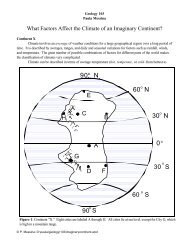
have lined up exactly with the terrain data; surprisingly, it did not. The shape files were
offset about 200 meters slightly west of north from the position of the digital elevation
model (see Figure 6.1). As stated in section 3.10 (page 74) USGS DEMs are referenced
using either the North American Datum of 1927 (NAD 27) or the North American Datum
of 1983 (NAD 83). The datum used for these DEMs was not specified, but the error
appeared as if the datum used in the terrain models was different from that of the GPS
data (which was collected using the World Geodetic System of 1984, or WGS84).
At first, a rubber sheeting approach was attempted to bring the two data types to
the same space, but this method brought with it significant systematic errors and was

169
Figure 6.1: Incongruent overlays due to conflicting references. The hill shaded relief
map of the Racetrack Playa (left) is based on the 7.5-minute Ubehebe Peak DEM,
which is referenced to NAD27. Overlain on this is the GPS vector file of the Racetrack’s
outline, based on WGS84. Note that the southern boundary of the playa is
clearly offset from the topography. The inset outlines the Grandstand; the large scale
detail (right) shows that the Grandstand (an easily recognizable feature) was about 200
meters farther northwest in the WGS-referenced data.
abandoned. Perusal of Arc/Info’s help screens clarified the problem, and suggested a
solution. Using Arc/Info’s Project function, the Ubehebe Peak DEM was transformed to
NAD83, thus shifting the pixels to coincide with the WGS84 vector files. Arc/Info did not
have a straightforward transformation application to convert from NAD27 to WGS84, so
NAD83 was used instead. NAD83 and WGS84 are virtually identical, both based on the
1980 Geodetic Reference System (GRS80); the more recent DMA-developed WGS84
spheroid carries calculations of the Earth’s shape to higher precision (Clarke, 1997).
Changing the ellipsoid of the DEM files thus resulted in an accurate overlay of the GPSmapped
data (Figure 6.2).

170
A
B
Figure 6.2: Comparison of NAD83 to WGS84. The Ubehebe Peak DEM was referenced
to NAD83 (upper left) from NAD27 (Figure 6.1). The Grandstand shape file
(white outline, inset A) is aligned with its 30 x 30 meter raster representation. The
south end of the playa (inset B) shows congruence with the dolomite cliffs.

171
6.2 Derived Raster Data
The Ubehebe Peak DEM was used to generate derivative slope and aspect data.
Since a digital terrain model is organized as a table whose cells correspond to local elevations,
pixel values may be computationally manipulated to yield applied data. A kernel
mask considers a small group of pixels at a time, and progressively moves throughout the
entire grid until every cell is assigned a value. This value may define the topographic gradient
of each 30 x 30 meter element (as in the case of a slope map), or the compass direction
of orientation for each 30 x 30 meter element (as in the case of an aspect map). These
processes are described (after Burrough, 1986), and illustrated below (see Figure 6.3).
Sample 3x3 array of 100 meter pixels
Altitude
Matrix:
100 130 140
Identifying
Kernel:
Z i-1,j+1
Z i,j+1
Z i+1,j+1
120 150 160
Z i-1,j
Z i,j
Z i+1,j
160 170 200
Z i-1,j-1
Z i,j-1
Z i+1,j-1
Figure 6.3: A 300 meter square of nine elevation values. This example is used to
derive slope and aspect of the central pixel below (Equations 6.1 and 6.2)
To derive the slope of any one pixel, the following equation is used:
TanG
=
( dZ)
( ----------- 2 ( dZ )
+
dX)
( ---------- 2
dY)
Equation 6.1
where:
[( dZ) ⁄ ( dX)
]ij , =
( Z ) 2Z i + 1,
j + 1 i + 1 , j
+ ( ) + ( Z ) Z i + 1 , j –
– ( 1 i – 1 , j + 1
) + ( 2Z ) +( Z )
i– 1,
j i – 1 , j – 1
----------------------------------------------------------------------------------------------------------------------------------------------------------------------------------------
8dX
Z i – 1,
j + 1
[( dZ) ⁄ dY]ij
,
( ) + ( 2Z ) Z ij , +
+ ( )– ( Z ) + ( 2Z ) +( Z )
1 i + 1 , j + 1 i – 1 , j – 1 ij , – 1 i + 1 , j –
= ------------------------------------------------------------------------------------------------------------------------------------------------------------------------------------------ 1
8dY
This is simply an expression of the Pythagorean Theorem. Substituting values to

172
solve for the central pixel in Figure 6.3,
( dZ)
-----------
( dX)
[ 140m + ( 2)160m + 200m] – [ 100m + ( 2)120m + 160m]
160m
= ------------------------------------------------------------------------------------------------------------------------------------------- = ------------ = 0.2
800m
800m
and:
( dZ)
----------
( dY)
[ 100m + ( 2)130m + 140m] – [ 160m + ( 2)170m + 200m]
–200m
= ------------------------------------------------------------------------------------------------------------------------------------------- = ---------------- = – 0.25
800m
800m
Substituting in Equation 6.1:
TanG = ( 0.2) 2 + (–
0.25) 2 = 0.32
so the slope of the central pixel in Figure 6.3 is derived by:
ArcTan( 0.32) = 17.75 o
To calculate the aspect of a pixel, the following equation is used:
(–dZ) ⁄ ( dY)
TanA = -----------------------------
Equation 6.2
( dZ) ⁄ ( dX)
applied:
This equation will yield a value for which the following decision rules must be
• if dZ/dX is negative and dZ/dY is negative: add 90° to the value derived by Eq. 6.2
• if dZ/dX is negative and dZ/dY is positive: subtract 90° from the value derived by Eq.
6.2
• if dZ/dX is positive and dZ/dY is negative: add 270° to the value derived by Eq. 6.2
• if dZ/dX is positive and dZ/dY is positive: subtract 270° from the value derived by
Eq. 6.2

173
So for the central pixel in Figure 6.3, we substitute the following values:
Aspect
[–(–0.25)]
= ArcTanA′ ------------------------- = 51.34 o
0.2
Since dZ/dX is positive, dZ/dY is negative, 270° is added to the outcome shown
above to yield a final value of 321.32°. A cursory examination of the subset shown in Figure
6.4 suggests that the central pixel must be sloping towards the northwest since the elevation
is lowest (100 meters) in the northwest corner and highest in the southeast (200
meters). When slope and aspect maps are developed by a GIS, these calculations are carried
out for every pixel in the grid, usually in a matter of seconds. Therefore, for a 1-
degree DEM more than 1.44 million separate calculations are conducted for the 1,201 x
1,201 array. The advantages of automated processes are apparent.
A slope map assigns hypsometric tints to inclination classes, thus indicating where
on a landscape the terrain is rugged, and where it is flat. Aspect maps code regions by the
direction in which each pixel or pixel cluster faces. These calculations are necessary precursors
to produce hill shaded relief images, in which reflectivity is inferred by these
derived data when combined with an operator-input azimuth and inclination for the sun.
Figure 6.4 shows a slope map of the Ubehebe Peak DEM, and Figure 6.5 shows an aspect
map of the same data set.

174
Ubehebe Peak 7.5-minute DEM
Slope Map
2500 0 2500 5000 Meters
Slope of Ubehebe
Peak DEM
(degrees)
0-4.9
5-9.9
10-14.9
15-19.9
20-24.9
25-29.9
30-34.9
35-39.9
40-44.9
45-49.9
50-54.9
55-59.9
60-64.9
Figure 6.4: Slope Map of Ubehebe Peak quadrangle. Note the Basin and Range
topography of generally north-south trending flat areas (controlled by structural
faults). Gently-sloping alluvial fans encroach the playa on the north, east and south.
This map was constructed with the USGS Ubehebe Peak DEM and ArcView’s Spatial
Analyst extension. The outline of the Racetrack Playa is the GPS vector data that was
collected in July 1996. UTM projection, zone 11.

175
Ubehebe Peak 7.5-minute DEM
Aspect Map
Aspect of Ube hebe
Peak DEM
(degrees)
Flat
(-1 )
North
(0-22.5,337.5-360)
Northeast
(22.5-67.5)
East
(67.5-112.5)
Southeast
(112.5-157.5)
South
(157.5-202.5)
Southwest
(202.5-247.5)
West
(247.5-292.5)
3000 0 3000 6000 Meters
Northwes t
(292.5-337.5)
No Da ta
Figure 6.5: Aspect map of the Ubehebe Peak quadrangle. When used in conjunction
with Figure 6.5, this map can give the viewer insight into the fault-blocked mountains
surrounding flat basins. Although the alluvial fans slope gently onto the playa floor,
their slope headings are nonetheless captured by this map.
The map was constructed with the USGS Ubehebe Peak DEM and ArcView’s
Spatial Analyst extension. The outline of the Racetrack Playa is the GPS vector data
that was collected in July 1996. Note the disparity in boundary between the playa
polygon and raster data. This is most likely due to the diffuse nature of the northern
and eastern borders. UTM projection, zone 11.

176
6.3 Correlating the Sliding Rock Trails to the Surrounding Terrain
Among the clearest patterns to emerge from the numerical data described in Chapter
5 is the favored trail heading in Octant 0, accounting for over 53% of all cumulative
motion. While other correlations were elusive at best, this general tendency for rocks to
slide to the north-northeast deserved further consideration. It had been established by
Sharp and Carey (1976) that prevailing winds in the area are from the south-southwest,
which is consistent with the preferential direction of movement observed in this survey.
Yet the existence of such a strong directional propensity may be influenced by the local
terrain and microtopography surrounding the lake bed. Figure 6.6 shows a contour map of
Figure 6.6: Contour map of south end of Ubehebe Peak DEM. Notice the
topographic corridors (indicated by gray arrows) to the south of the Racetrack.
Contours constructed as vector features with a 50-meter interval using
ArcView 3.0’s Spatial Analyst.

177
the south end of the playa, highlighting saddles through which air may be channeled and
directed onto the playa. Figure 6.7 shows a perspective view of the southwest saddle
where two corridors converge, serving to concentrate airflow directly onto the sliding rock
field.
There is a high degree of parallelism between the major heading component of
most trails and these natural airways. To statistically test the surrounding topography’s
influence on rock motion, the aspect (compass direction of slope orientation) of the local
terrain was examined.
6.3.1 Neighborhood Aspect Analysis
The sliding rock field is concentrated at the south end of the Racetrack, so the
Figure 6.7: Perspective view of the southwest sector of the Racetrack Basin. The two
arrows in the extreme southwest corner of Figure 6.7 are shown here as would be seen
from the southern playa shoreline. If air is channeled through these saddles, currents
converge onto the flat Racetrack floor.
This image is based on the one-degree USGS Death Valley-West DEM, processed
as a grid using Arc/Info and imported into ERDAS Imagine version 8.2.

...
178
influence of winds may be somewhat limited in scope. Since all rock trails were digitized,
each start point was known (see Table G4 in Appendix G); each start point represents a
place where air forces exceeded a rock’s coefficient of static friction thereby propelling
the rock. The zone on the playa that encompassed all start points is a bounding “neighborhood”
polygon of every such point in the data set, and is the area on which further studies
are based (see Figure 6.8).
To test whether the aspect of the terrain elements within a limited distance from
this “neighborhood” polygon had influence over rock motion, a second polygon was constructed
with a border 2000 meters from that of the bounding polygon. The extent of this
demarcation is illustrated in Figure 6.9. The 2000 meter buffer was used to filter any ter-
.
. .
.
.
..
... .
.. .. ..
....
.. . ....
. ..
..
.. .
..... ..
.... .
. .. . ... ..
..
..
.
.
.
Figure 6.8: Bounding polygon of sliding rock start points. The dark gray shape file is
superimposed on a hill shaded relief image of Racetrack Basin. White dots indicate
trail origin points.

179
2000 m.
Key:
Fla t (-1 )
North (0-22.5,337.5-360)
Northeast (22.5-67.5)
East (67.5-112.5)
Sou thea s t (1 12 .5-15 7.5 )
South (157.5-202.5)
Southwest (202.5-247.5)
We s t (2 47 .5 -29 2.5)
No rthwe s t (2 92 .5-33 7.5 )
0 1000 2000 Me te rs
Figure 6.9: Buffer zone surrounding the bounding polygon. The hillshaded relief
image (top) shows the extent of the elevation data included in visibility analyses (see
section 6.32). The aspect map (bottom) shows the same buffer zone; this time the pixels
are coded for azimuth of inclination.
rain data beyond that distance from the rock field. Once the DEM was filtered, an aspect
data set was created from this subset. The resultant “clipped” aspect map was the base
map for the next phase of analysis.

180
visible
invisible
invisible
visible
viewpoint
Figure 6.11: Intervisibility using ray tracing. (After Clarke, 1995)
6.3.2 Viewshed Analyses
The rocks at Racetrack Playa lie on a flat plane, but are surrounded by intricate
landforms. Air is forced through natural channels, but each rock may be subject to slight
differences in wind velocity based on its location relative to the fringing topography.
Given a digital cartographic representation of a terrain surface and a single point
on the surface, the set of regions that are visible from that point describe intervisibility
(Clarke, 1995). Intervisibility is determined by a method known as ray tracing, and is
illustrated in Figure 6.11. The viewshed, or 360 o panorama of the visible terrain around
each rock is a function of its placement and height above the surface. On a perfectly flat
terrain, a viewshed would extend to the visible horizon in all directions. Any substantial
relief such as a mountain acts as a barrier to the panorama, and also as a shield to air currents
at shorter ranges. Processing viewsheds for representative rocks could establish the
existence of significant variations in the terrain in the neighboring buffer zone, and hence
associated airflow potentials.

181
For this study, the start points of twelve rocks were selected. The subset of rocks
was chosen based on several criteria: spatial distribution on the playa; representation of a
range of trail straightness ratios; representation of a range of trail lengths; representation
of a range of rock sizes. Selection rationalization for each rock is listed in Table 6.1.
.
Table 6.1: Twelve-rock Visibility Subset Selection Criteria
Rock
Number/Name
UTM Coordinates of
Start Point
Easting
(X)
Northing
(Y)
Rationale
031 Jacki 450131.0 4057974.5 Although starting nearly 37 meters apart
032 Amelia 450099.9 4057956.3
on the playa, these trails end in highly parallel
“scribbles.”
045 Karen 450025.4 4058639.4 One of the three largest rocks; situated at
the northwestern neighborhood limit.
050 Alice 450235.0 4058450.5 The second most crooked trail (0.271
straightness quotient).
063 Marietta 450215.9 4057719.6 The most southerly start point.
069 Sandra 450013.9 4057625.9 An extreme southwesterly start point.
073 Claudia 450125.1 4058042.0 The most crooked trail (0.187 straightness
quotient).
080 Sheryl 450199.6 4057998.8 The straightest trails of appreciable
084 Jospehine 450237.5 4057784.0
length * (0.997 straightness quotient).
140 Debbie 450726.8 4058005.2 An extreme southeasterly start point.
141 April 450953.3 4058866.9 The most northeasterly start point.
145 Diane 450444.5 4057957.6 The longest trail (881 meters).
*139 Agnes is the straightest trail, but it measures only 6 meters in length. As a result, 080 Sheryl
and 084 Josephine (with trail lengths of 26 and 84 meters, respectively) were included instead.
Each of the twelve trail origin points were saved as point coverages using Arc/Info

182
generate. Point files were cleaned and projected to UTM. The Ubehebe Peak DEM was
cropped using the Arc command latticeclip: the polygon coverage of the 2000-meter
buffer zone acted as a “cookie cutter.” The resulting DEM extended 2000 meters beyond
the limit of the bounding polygon in all directions, and was named .
Using each of the twelve point coverages individually, the Arc command visibility
computed the 360 o viewshed for each start point. The usage for this command, using
Amelia as an example is:
where:
visibility point grid
• is the 2000-meter buffer cropped DEM-derived aspect map,
• is the point coverage of Amelia’s origin,
• “point” specifies that the viewshed will be based on one point (as opposed to a line),
• is the name of the viewshed grid file generated,
• “grid” specifies that the output file is a raster grid.
It should be noted that this process is computationally intensive and quite time-consuming.
When the grids were output to ArcView their associated data base files were
exported to Excel. The original clipped DEM encompassing the 2000-meter buffer zone
contained 22,749 30x30-meter pixels. Since this value was known, as were the total number
of visible pixels in each rock’s viewshed, the “visibility ratio” of each rock was computed.
The quotient of the rock’s visible pixels to the total number of pixels in the
buffered grid describes the relative intervisibility for that rock before it started moving.
Table 6.2 shows the relative viewsheds for the twelve representative rocks.

183
Table 6.2: Number of Pixels Visible/Invisible to Twelve Representative Rocks
Rock Name/
Number
Number of
Pixels
Visible
Number of
Pixels
Invisible
Visibility
Quotient
Alice 050 15205 7544 .6684
Amelia 032 14595 8154 .6416
April 141 13354 9395 .5870
Claudia 073 14727 8022 .6474
Debbie 140 16406 6343 .7212
Diane 145 13515 9234 .5941
Jacki 031 14517 8232 .6381
Josephine 084 13036 9713 .5730
Karen 045 15834 6915 .6960
Marietta 063 11972 10777 .5263
Sandra 069 12452 10297 .5474
Sheryl 080 14339 8410 .6303
As is evident in Figure 6.11, the rocks selected for the visibility studies describe an
approximately normal distribution of visibility profiles. A cursory analysis of Table 6.2
shows that the longest trail (Diane) had one of the smallest number of visible viewshed
pixels at its start point. Given this possible link to total intervisibility area and trail character,
several regression analyses were implemented. The results of those scatter plots are
presented in Table 6.3.

184
4
4
3
3
Frequency
2
1
2
2
1
0
0.50-0.55 0.55-0.60 0.60-0.65 0.65-0.70 0.70-0.75
Visibility Quotient
Figure 6.11: Frequency distribution of visibility quotients for representative rocks.
Table 6.3: Results of Selected Visibility-Related Regression Analyses
X variable
Y variable
Relationship
(+ = direct;
- = inverse)
Correlation
Coefficient
(r 2 )
Number of
Total Visible
Pixels in
Viewshed
Straightness Quotient of Trail - 0.1679
Distance to Springs of Trail Start Point - 0.0842
Direct Trail Length - 0.0135
Total Trail Length + 0.0061
Relationships between trail character parameters and number of viewshed pixels
were weak. However, the analyses above weighted all visible pixels equally. Since the
goal of this study was to associate qualities of trails with the surrounding terrain, further
intervisibility area details were needed. An aspect analysis of the DEM subset
was generated, and named . The twelve raster files resulting from the visibility

185
analysis function (see “visibility . . .” on page 182) were converted to polygons
using Arc’s gridpoly function. All twelve coverages were named ,
projected to UTM, and then cleaned. These coverages were in turn used as “cookie cutters”
on the cropped aspect map, “clipasp.” The command for Amelia, for example was:
where:
latticeclip
• is the grid of aspect-coded pixels to be cropped,
• is the viewshed polygon,
• is the output viewshed grid
The resulting twelve rocks’ “-vis” grids were raster files of the aspect of every visible
pixel in that rock’s viewshed, before it started moving to its current location.
The tabular data from these manipulations were exported to Microsoft Excel. The
spreadheets, as exported by ArcView, consisted of two columns, one for the compass
heading and the other for the total number of pixels in the viewshed with that orientation
for each rock. There were up to 361 rows for each rock, one row for the flat pixels in the
viewshed (labeled “-1 o ”), and one row and associated number of pixels for each compass
heading (1 o to 360 o ).
Once the spreadsheet was constructed, pixels were “clumped” into eight groups to
match the octant categories already defined. Table 6.4 shows the summation limits.

186
Table 6.4: Aspect Designation by Octant
Octants
0 1 2 3 4 5 6 7
Inclusive Headings 1-45 46-
90
91-
135
136-
180
181-
225
226-
270
271-
315
316-
360
The data were summed further to produce groups of the four cardinal compass
directions, and again to those offset by 45 o . Table 6.5 shows these distributions.
Table 6.5: Aspect Designation by Quadrant
Quadrants
N E S W NE SE SW NW
Inclusive Headings 1-45;
316-360
96-
135
136-
225
226-
315
1-
90
91-
180
181-
270
271-
360
A summary of the total number of visible pixels by Octant (Table 6.5) follows.

187
Table 6.5: Number of Visible Pixels in Viewshed of Rock, by Octant
Rock
Name/
Number
Octants
0 1 2 3 4 5 6 7
Total Inclined
Pixels
Flat Pixels
Total Pixels in
Viewshed
Alice
050
Amelia
032
April
141
Claudia
73
Debbie
140
Diane
145
Jacki
31
Josephine
84
Karen
45
Marietta
63
Sandra
69
Sheryl
80
857 2086 1612 324 515 1562 1575 1269 9800 5405 15205
717 2054 1602 333 495 1633 1402 954 9190 5405 14595
746 2155 1616 300 381 932 1137 884 8151 5203 13354
740 2059 1604 332 496 1623 1422 1041 9317 5410 14727
898 2089 1489 354 621 1939 2142 1443 10975 5431 16406
620 2083 1602 317 431 1273 1176 710 8212 5303 13515
720 2056 1600 331 488 1618 1367 935 9115 5402 14517
510 2036 1589 325 458 1372 955 445 7690 5346 13036
873 2090 1526 321 566 1750 1898 1387 10411 5423 15834
363 1988 1540 318 436 1207 720 177 6749 5223 11972
492 1919 1532 322 464 1375 714 378 7196 5256 12452
714 2055 1601 331 482 1525 1316 922 8946 5393 14339

188
as follows:
The pixel counts for octants were added together defining viewsheds by quadrant,
• Σ pixels in Octants 7 + 0 describe visible North-facing slopes,
• Σ pixels in Octants 1 + 2 describe visible East-facing slopes,
• Σ pixels in Octants 3 + 4 describe visible South-facing slopes,
• Σ pixels in Octants 5 + 6 describe visible West-facing slopes,
• Σ pixels in Octants 0 + 1 describe visible Northeast-facing slopes,
• Σ pixels in Octants 2 + 3 describe visible Southeast-facing slopes,
• Σ pixels in Octants 4 + 5 describe visible Southwest-facing slopes,
• Σ pixels in Octants 6 + 7 describe visible Northwest-facing slopes.
These totals may be found in Tables H1 and H2 in Appendix H.
6.3.3 Trail Heading Correlations to Surrounding Visible Topography
Motion of the rocks is inferred by the pattern of their trails: Table G5 in Appendix
G lists motion by octants; Table G6 in Appendix G lists the percentages of a rock’s route
in each octant. As noted by Figures 5.27 (page 153) and 5.28 (page 154) the greatest
directional component for the majority of trails was in Octant 0 (north-northeast). When a
similar analysis is conducted on the representative samples’ visible pixel aspects, it is evident
that the heading of surrounding terrain elements are not random and are related to the
design of the trails. Table H3 in Appendix H shows the percentage of visible pixels per
octant and per quadrant of each of the rocks, excluding the flat terrain. Figure 6.12 shows
the viewshed means for all rocks.
For the twelve representative rocks, percentages of direction components per trail
and orientation of pixel elements per viewshed were calculated, by quadrant. Table H4 in
Appendix H shows the complete data for individual trails and viewsheds. These data were
then averaged by quadrant (Table 6.6). A comparison of the sampled rocks’ mean trail
segment headings to their visible pixel aspects shows some interesting patterns.

189
25%
23.73%
20%
18.24%
16.85%
Percent of Visible Pixels
15%
10%
5%
7.71%
3.76%
5.55%
14.61%
9.56%
0%
0 1 2 3 4 5 6 7
Octant
Figure 6.12: Mean percentage of aspects visible to representative rocks, by octant.
.
Table 6.6: Pixel Aspect Means for Sampled Rocks’ Viewsheds and Corresponding
Trail Heading Means, by Quadrant
North East South West
Aspect of
Viewshed
Pixels
Trail Heading
Components
17.26% 41.97% 9.31% 31.46%
66.36% 6.38% 10.92% 16.34%
Northeast Southeast Southwest Northwest
Aspect of
Viewshed
Pixels
Trail Heading
Components
31.44% 22.00% 22.40% 24.17%
44.41% 13.41% 2.97% 39.22%

190
There is a noticeable inverse relationship between aspect of viewsheds and trail
headings. Particularly in the cardinal directions (top) Table 6.6 shows that high values in a
particular quadrant for pixel aspects corresponded to low values for trail headings, and
vice versa. The relationship in the offset quadrants (bottom) are more diffuse.
When percentages for complementing quadrants are summed and compared, the
results suggest a significant relationship between trail character and terrain. Figure 6.13
shows the correspondence.
100%
90%
80%
70%
60%
50%
40%
30%
20%
10%
0%
93.17%
73.43%
26.57%
6.83%
53.84%
52.03%
46.16%
47.97%
N-S E-W NE-SW NW-SE
Sector
Trails
Aspects
Figure 6.13: Comparison of pixel aspects to trail component headings for averages of
twelve representative rocks.
The trails show a directional preference to the quadrants orthogonal to the majority
of the pixel aspects’ orientations. In other words, a preponderance of east- or westfacing
slopes appears to be correlated with the general north-south plans of the trails. This
is particularly evident of north-south, east-west correlations in Figure 6.13.

191
To check the interdependence of trails to their surrounding orthogonal terrain elements
t-Tests were conducted. Tests on whether the paired data support a null hypothesis
(i.e., there is no relationship between the trails’ directions and orientation of the surrounding
slopes) allowed the null hypothesis to be rejected at the 95% confidence level
(α=0.05). The results of two such comparisons are shown in Table 6.7.
Table 6.7: Results of t-Tests for Terrain-Trail Paired Data
NE-SW
Trails
NW-SE
Terrain
N-S Trails
E-W Terrain
Mean 51.76 46.16 78.95 73.43
Variance 1344.38 8.99 819.88 11.96
Observations 12 12 12 12
Pearson Correlation
Hypothesized
Mean Difference
0.117 -0.550
0 0
df 11 11
t Stat 0.532 0.624
P(T