mathematica introduction - School of Maths and Stats Local Site

IntroFowkes.nb 1
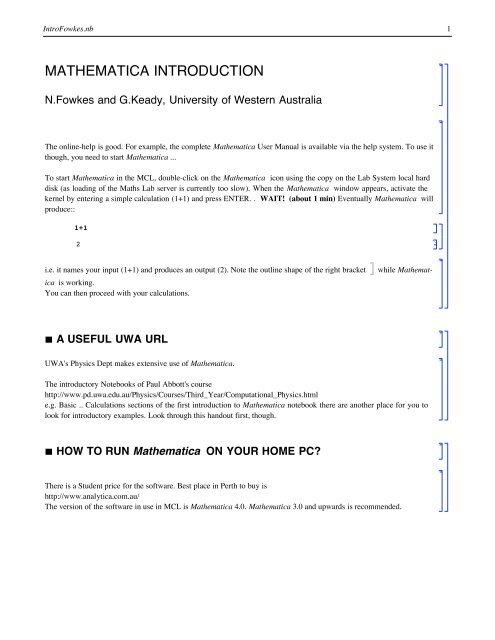
MATHEMATICA INTRODUCTION
N.Fowkes and G.Keady, University of Western Australia
The online-help is good. For example, the complete Mathematica User Manual is available via the help system. To use it
though, you need to start Mathematica ...
To start Mathematica in the MCL, double-click on the Mathematica icon using the copy on the Lab System local hard
disk (as loading of the Maths Lab server is currently too slow). When the Mathematica window appears, activate the
kernel by entering a simple calculation (1+1) and press ENTER. . WAIT! (about 1 min) Eventually Mathematica will
produce::
1+1
2
i.e. it names your input (1+1) and produces an output (2). Note the outline shape of the right bracket ] while Mathematica
is working.
You can then proceed with your calculations.
‡ A USEFUL UWA URL
UWA's Physics Dept makes extensive use of Mathematica.
The introductory Notebooks of Paul Abbott's course
http://www.pd.uwa.edu.au/Physics/Courses/Third_Year/Computational_Physics.html
e.g. Basic .. Calculations sections of the first introduction to Mathematica notebook there are another place for you to
look for introductory examples. Look through this handout first, though.
‡ HOW TO RUN Mathematica ON YOUR HOME PC
There is a Student price for the software. Best place in Perth to buy is
http://www.analytica.com.au/
The version of the software in use in MCL is Mathematica 4.0. Mathematica 3.0 and upwards is recommended.

IntroFowkes.nb 2
‡ HELP
1. For beginners, the most useful first item is the Getting Started from the Help menu and going to the "Tour of Mathematica"
there.
2. For help with individual functions, for example with a function whose name begins with "Nam", type
Nam*
Nam* for more help,
N* for help on all of the functions beginning with N..
3. For help on mathematical functions, use the Function Browser under the Help menu.
4. To stop a calculation use `Control,' .
5. To quit, select Quit from the File menu.
6. Balloon Help can be used in connection with what is on the menus in the FrontEnd.
‡ ELEMENTARY CALCULATIONS
Pi+2^2+1/2+3 4
33
ÅÅÅÅÅÅÅ
2 + p
An exact calculation. Note that Pi cannot be written exactly. Note that a space (or *) denotes multiplication. Note also
that an initial capital letter is used for Mathematica functions. You should use small letters for the expressions you
introduce. Enter needs to be pressed to complete the calculation, and labels Out[1], In[1] are introduced by the program.
To get a numerical approximation use:
N[%]
19.6416
N evaluates the expression approximately. % denotes the previous output. %% the output before this etc. %n denotes
Out[n]. Note that a square bracket [] is used for arguments of functions.
ü VARIABLES, EQUATIONS
eq=x^2 +b*x +1
1 + b x + x 2
Solve[eq==0,x]
99x Ø ÅÅÅÅ
1 è!!!!!!!!!!!!!!!
I-b - -4 + b
2 2 M=, 9x Ø ÅÅÅÅ
1 è!!!!!!!!!!!!!!!
I-b + -4 + b
2 2 M==

IntroFowkes.nb 3
Note the == used for an equation. The single = assigns the value x^2 +b*x +1 to eq . Note that the outcome of
Solve is presented as a list, the 2 solutions, in curly {} brackets. We can now input a particular numerical value of b (9
say) (by using the operator /. and b->9 and evaluate approximately use the N operator:
N[%] /. b->9
88x Ø -8.88748

IntroFowkes.nb 4
Show[p1,Frame->True]
1
0.5
0
-0.5
-1
-3 -2 -1 0 1 2 3
Ü Graphics Ü
The ``option '' Frame introduces a frame about the graph. Use Options to see about options. For surface and contour
maps ask for help about Plot3D, ParametricPlot3D, ContourPlot. Also check up on the Show, AxesLabels,
PlotLabel, Viewpoint Options.
ü LINEAR ALGERA
m={{a,b},{c,d}}
88a, b

IntroFowkes.nb 5
ans =DSolve[ {
y''[t] +40*y'[t] +625*y[t]==100*Cos[10*t],
y[0]==0, y'[0]==0 },
y[t], t]
99y@tD Ø ÅÅÅÅÅÅÅÅÅ
1
697 ‰-20 t J84 ‰ 20 t Cos@10 tD - 84 Cos@15 tD + 64 ‰ 20 t Sin@10 tD - ÅÅÅÅÅÅÅÅÅÅ
464
3
yans = y@tD ê. ans@@1DD ;
Plot@yans, 8t, 0, 1.2

IntroFowkes.nb 6
eq=x^2 +b*x +c
c + b x + x 2
the expression for eq we want.
4. Equations use a double equals sign.
There is much more to Mathematica than this. There are details concerning Palettes and Notebooks you may find
useful. Whole 'interactive engineering handbooks' have been prepared using these facilities.
However, in M28n our approach is to encourage you to learn the CAS from applying it to help you solve typical
'engineering maths' problems, and to provide a gentle introduction via a systematic set of labs. These are at
http://maths.uwa.edu.au/~keady/M28p
in a password protected area. The login is m28n, the password is m28n****