Modeling and simulation

Modeling and simulation
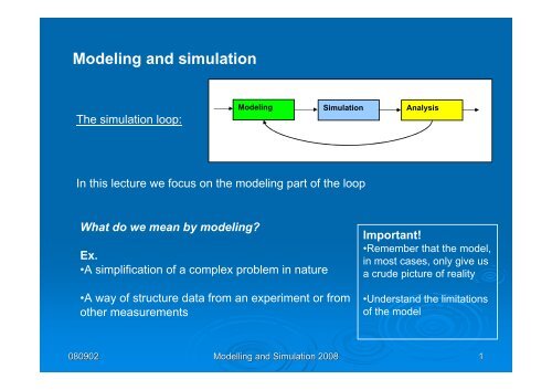
The simulation loop:
Modeling Simulation Analysis
In this lecture we focus on the modeling part of the loop
What do we mean by modeling
Ex.
•A simplification of a complex problem in nature
•A way of structure data from an experiment or from
other measurements
Important!
•Remember that the model,
in most cases, only give us
a crude picture of reality
•Understand the limitations
of the model
080902 Modelling and Simulation 2008 1

Predator-prey systems
- Ecological examples
Disaster of Lake Victoria
•The lake supported hundreds of small fishing
communities fishing several species
•A new big fish was introduced in the lake
•Result: The new fish wiped out many other
speices….
•More: Diseases, felling of trees for fuel…
Murray J.D., “Mathematical biology”, Springer-Verlag, 1993
080902 Modelling and Simulation 2008 2

A simple predator-prey system
Our toy system: An island where two species lives, predators (foxes)
and preys (rabbits)
Our first assumptions:
•The foxes eat rabbits and breed
•The rabbits eat grass and breed
•The area is limited, but the grass grows faster than the rabbits can
eat
080902 Modelling and Simulation 2008 3

Let us build a mathematical model
(Lotka-Volterra system)
R = Number density of rabbits
F = Number density of foxes
1. Only rabbits, inifite food supply
8 x 105 Prey model ODE
6
Rabbits
dR =
dt
aR
a
= growth rate
4
2
0
0 5 10 15 20
Limited food supply
dR
dt
⎛ = a⎜
1−
⎝
R ⎞
⎟R
K ⎠
600
400
Prey model ODE
Rabbits
K
= Carrying capacity
200
0
0 5 10 15 20
080902 Modelling and Simulation 2008 4

dR
dt
⎛ R ⎞
a⎜1 − ⎟R
= aR−
⎝ K ⎠
R
K
2
Steady state solutions:
R1 = 0 Unstable
R
2
=
K
=
0 5 10 15 20
Stable
600
400
200
0
Prey model ODE
Rabbits
080902 Modelling and Simulation 2008 5

2. Only foxes
250
200
Predator-Prey model ODE
Foxes
dF
dt
= − dF
d
= death rate
150
100
50
3. Rabbits and foxes
0
0 5 10 15 20
Assumptions:
More rabbits => more food for foxes => foxes tends to breed more
More foxes => more rabbits are killed
Fox model:
Rabbit model:
dF
dt
dR
dt
= −dF
+ cRF
= aR−bFR
Lotka-Volterra equations
080902 Modelling and Simulation 2008 6

Solving an ODE-system using Matlab
⎧dR
⎪ dt
⎨
⎪dF
⎩ dt
=
=
aR − bFR
cRF − dF
a ≈ the rabbits growth rate
bF ≈ the rabbits death rate
cR ≈ the foxes growth rate
d ≈ the foxes death rate
To solve this ODE-system we have to use a numerical method.
In the software Matlab there is a collection of methods that are easy
to use.
Note: Different choices of parameters may take longer/shorter to
solve depending on numerical method
Later in this course you will learn how to choose a numerical method
best fitted to solve a specific problem
080902 Modelling and Simulation 2008 7

Typical solutions…
1500
Predator-Prey model ODE
Rabbits
Foxes
Predator-Prey Trajectory a=0.4, b=0.001, c=0.001, d=0.9
1000
800
1000
500
Foxes
600
400
200
0
0 20 40 60 80 100
0
0 500 1000 1500
Rabbits
1000
800
Predator-Prey model ODE
Rabbits
Foxes
Predator-Prey Trajectory a=0.4, b=0.004, c=0.004, d=0.9
800
600
600
400
200
Foxes
400
200
0
0 20 40 60 80 100
0
0 200 400 600 800 1000
Rabbits
080902 Modelling and Simulation 2008 8

Limitations of our model
• Infinite grass supply leads to exponential growth of the rabbit
population if no foxes are alive
• The fox population can grow without saturation
• Only two species…
080902 Modelling and Simulation 2008 9

More realistic predator-prey systems
Finite grass resources
⎛
a → a ⎜1
−
⎝
R
K
⎞
⎟
⎠
800
600
400
Predator-Prey model ODE
Rabbits
Foxes
Foxes
Trajectory a=0.4, b=0.004, c=0.004, d=0.9, K=800
800
600
400
200
200
0
0 20 40 60 80 100
0
0 200 400 600
Rabbits
Finite prey consumption
RF
→
1
RF
+
R
S
5000
4000
3000
2000
1000
Predator-Prey model ODE
Rabbits
Foxes
Foxes
Trajectory a=0.4, b=0.004, c=0.004, d=0.9, S=2500
5000
4000
3000
2000
1000
S
= Fox eating saturation
0
0 20 40 60 80 100
0
0 1000 2000 3000 4000 5000
Rabbits
080902 Modelling and Simulation 2008 10

Results from a model with both limited grass supply and
limited prey consumption
800
600
Predator-Prey model ODE
Rabbits
Foxes
Trajectory a=0.4, b=0.004, c=0.004, d=0.9, K=800, S=600
600
500
400
400
200
0
0 20 40 60 80 100
Foxes
300
200
100
0
0 200 400 600 800
Rabbits
080902 Modelling and Simulation 2008 11

Predator-prey laboration 1
Exercises
1. Implement and solve the standard predator-prey equations
2. Add limited grass supply (see model above)
3. Add limited prey consumption (see model above)
4. Add a third species
080902 Modelling and Simulation 2008 12

So, what is Matlab
•A simple programming environment
•Mathematical modules (ODE solvers, statistical tools, algebraic tools…)
•Graphics
•Possibility to connect to external simulations
How do we use Matlab
080902 Modelling and Simulation 2008 13

% A Matlab code for solving the Predator-Prey system
clear, clear global
global a b c d
%Define equation coefficients
a=0.4; %Rabbit growth rate
b=0.001; %Rabbit death coefficient
c=0.001; %Fox growth coefficient
d=0.9; %Fox death rate
% Define the variables used as inputs in the ODE-solver
t0=0;
tmax=1000;
Ntot=1000;
p=0.4;
RabbitIni=(1-p)*Ntot;
FoxIni=p*Ntot;
options = odeset('RelTol',1e-4,'AbsTol',[1e-7 1e-7]);
Save as PredatorPrey.m
Save as rabbitfox.m
function dy = rabbitfox(t,y);
dy = zeros(2,1);
global a b c d
% Solve ODE system
[T,Y] = ode45(@rabbitfox,[t0 tmax],[RabbitIni FoxIni],options);
% Definition of the ODE
% y(1) = Number of rabbits
% y(2) = Number of foxes
%Plot
figure(1)
dy(1) = a*y(1) - b*y(2)*y(1);
plot(T,Y(:,1),'r')
hold on
dy(2) = c*y(1)*y(2) - d*y(2);
plot(T,Y(:,2),'--b')
legend('Rabbits','Foxes')
title('Predator-Prey model ODE')
080902 Modelling and Simulation 2008 14

General remarks about ODE systems (a very short overview…)
We have seen plots like those to the right
Note, for example, the spiral motion into a single point…
Foxes
1000
800
600
400
y j y
200
800
600
Predator-Prey model ODE
Rabbits
Foxes
Trajectory a=0.4, b=0.004, c=0.004, d=0.9, K=800
800
600
0
0 500 1000 1500
Rabbits
400
Foxes
400
800
200
200
600
0
0 20 40 60 80 100
0
0 200 400 600
Rabbits
Foxes
400
200
Such a point is called a fixed point and represents
a steady state situation:
dR
dt
dF
= 0 , =
dt
0
(The unmodified case)
⎧R
= F
⎨
⎩R
= d
=
/ c,
0
F
=
a / b
Foxes
0
0 200 400 600
Rabbits
5000
4000
3000
2000
1000
0
0 1000 2000 3000 4000 5000
Rabbits
080902 Modelling and Simulation 2008 15

Typical state space trajectories near fixed points
Node Repellor Spiral
node
Spiral
repellor
Cycle
R = F = 0 is a saddle point
R = d / c,
F = a / b is a cycle
Saddle
point Hilborn R.C., “Chaos and nonlinear dynamics”, Oxford University Press Inc., 1994
080902 Modelling and Simulation 2008 16

State space transitions
Ex.
•If the parameters in an ODE-system are changed, we can have a
transition from one type of state space behavior to another.
•Such a transition is called a bifurcation
•In order to study bifurcation it is very useful to write the ODE in nondimensional
form. In the unmodified case we make the following
substitutions:
⎧dF
d
⎪ =
dt d
⎨
⎪ ⎛
− dF = − d
⎪
⎜
⎩ ⎝
cR bF
u = , v = , τ = at,
α =
d a
( τ / a)
⎛
⎜
⎝
av
b
av ⎞
⎟
b ⎠
⎞
⎟
⎠
= −
=
a
b
ad
b
2
dv
dτ
2
a
v = −
b
αv
d
a
Non-dimensional form
⎧du
⎪ dt
⎨
⎪dv
⎩ dt
=
= α
( 1−
v)
u
( u −1)
ONLY ONE PARAMETER!!
v
080902 Modelling and Simulation 2008 17

Chaotic trajectories
Poincaré-Bendixon Theorem says something like:
(works only in 2D)
Assume that we have a bounded system…
Then the trajectory only have two choices:
1. The trajectory approaches the fixed point
2. The trajectory approaches a limit cycle (a cycle
which attracts all neighboring trajectories)
A further important result based on this theorem is that we need at
least three dimensions in order to have chaos
080902 Modelling and Simulation 2008 18

Further reading for those who are interested:
1. N. Britton, “Essential Mathematical Biology”, Springer-Verlag,
2003
2. Murray J.D., “Mathematical biology”, Springer-Verlag, 1993
3. Hilborn R.C., “Chaos and nonlinear dynamics”, Oxford University
Press Inc., 1994
080902 Modelling and Simulation 2008 19

An other way to simulate predator-prey
system…
•The ODE model above describes the evolution of the
population densities
• We do not get any information about dynamics of individual
animals
•Is it possible to construct a simulation of individuals
that give us similar results as the ODE model
080902 Modelling and Simulation 2008 20

Cellular Automata and Agent Based Models
Game of Life, John Conway (1970)
Ex
-Individuals are distributed on a grid
-Each individual has a well defined neighborhood
-Simple rules stating the birth and death of
individuals
-The whole grid is updated each time step
Simple rules on microscopic level (individuals)
=> Complex behavior on macroscopic scales
080902 Modelling and Simulation 2008 21

Predator-Prey simulation using a Cellular Automata (CA)
080902 Modelling and Simulation 2008 22

1200
1000
Foxes
Rabbits
1200
1000
800
800
600
400
Rabbits
600
400
200
200
0
0 1000 2000 3000 4000 5000
0
0 200 400 600
Foxes
50
Initial
50
Final
40
40
30
30
20
20
10
10
0 10 20 30 40 50
0 10 20 30 40 50
080902 Modelling and Simulation 2008 23

1500
1000
500
Foxes
Rabbits
Rabbits
1500
1000
500
0
0 2000 4000 6000
50
40
30
20
10
Initial
0 20 40
0
0 200 400 600
Foxes
50
40
30
20
10
Final
0 20 40
080902 Modelling and Simulation 2008 24

Predator-prey laboration 2
Exercises
1. Implement a simulation, based on individuals, with following properties:
- One predator and one prey
- The species should be able to move around on a rectangular grid
- Each individual should have limited energy capacity (they need to eat)
- The behavior of individuals should be controlled by SIMPLE rules
2. Add limited grass supply
3. Add limited prey consumption
4. Add a third species
080902 Modelling and Simulation 2008 25