Nonequilibrium fluctuation-dissipation theorem of ... - LY Chen

More documents

Recommendations

Info

144113-2 L. Y. Chen J. Chem. Phys. 129, 144113 2008 Langevin equation in Eq. 3. If the Stratonovich scheme were adopted, would have a very complex dependence on the coordinates through V n+1 and F n+1 . When that complex dependence is correctly accounted for, the Stratonovich scheme should agree exactly with the Ito scheme. 9 Considering the dynamics of the system is Markovian, we have the probability for transition along a given path xt=x 0 ,x 1 ,...,x N from state A x 0 =x A to state B x N =x B as follows: Px 0 ,t 0 x 1 ,t 1 ¯ x N ,t N N−1 = p e x A Px n ,t n x n+1 ,t n+1 n=0 = 1 N−1 mxn+1 − x Np ex A exp− n + V n dt − F n dt 2 , n=0 4mk B Tdt where p e x A =exp−Vx A /Z A is the equilibrium probability distribution of the system when it is constrained to the 5 macroscopic state A. Z A =exp−G A is the partition function and G A is the free energy of that macroscopic state. 1/k B T. The system is driven from state A to state B by the external force Ft=F 0 ,F 1 ,...,F N . The following question has been asked but not answered correctly in the current literature: What is the probability for the system to take the exact reverse path x˜t =x N ,x N−1 ,...,x 0 if the external driving force is tuned backward in time, F˜ t=F N ,F N−1 ,...,F 0 Answering this question correctly requires particular attention to the subtle stochastic nature of the Brownian dynamics. Resembling exactly Eq. 4, the transition probability between state x N−n at time t n and state x N−n−1 at time t n+1 is Px N−n ,t n x N−n−1 ,t n+1 = 1 exp− mx N−n−1 − x N−n + V N−n dt − F N−n dt 2 4mk B Tdt . The probability for transition along the reverse path x˜t =x N ,x N−1 ,...,x 0 is 6 N−1 Px N ,t 0 x N−1 ,t 1 ¯ x 0 ,t N = p e x B n=0 Px N−n ,t n x N−n−1 ,t n+1 = 1 N−1 mxN−n−1 − x Np ex B exp− N−n + V N−n dt − F N−n dt 2 , n=0 4mk B Tdt where p e x B =expG B −Vx B is the equilibrium probability of the system when constrained to the macroscopic state B. The relationship between the probabilities along the forward and reverse paths will become clear once we substitute the dummy index n in the sum on the second line of Eq. 7, l=N−n−1. Then, 7 Px N ,t 0 x N−1 ,t 1 ¯ x 0 ,t N = 1 N−1 mxl − x Np ex B exp− l+1 + V l+1 dt − F l+1 dt 2 . 8 l=0 4mk B Tdt Note that the indices are in different order than those of Eq. 5. The ratio between the two probabilities can be found as Px 0 ,t 0 x 1 ,t 1 ¯ x N ,t N Px N ,t 0 x N−1 ,t 1 ¯ x 0 ,t N = p N−1 ex A p e x B exp xn+1 − x − n V n − F n − x n − x n+1 V n+1 − F n+1 . 9 2k B T n=0 In deriving the above equation, we made use of the fact that dt is infinitesimal so that exp− V N − F N 2 − V 0 − F 0 2 =1. 10 4mk B T dtdt→0 Examining the differentials in the exponent on the right hand side of Eq. 9, we note that the internal force V terms lead to the potential energy differences between states A and B as follows: N−1 n=0 N−1 n=0 N−1 x n+1 − x n V n = Vx n+1 − Vx n = Vx B − Vx A , n=0 11 N−1 x n − x n+1 V n+1 = Vx n − Vx n+1 = Vx A − Vx B . n=0 However, the external driving forces are not conservative and their terms have to be dealt with explicitly. Now we have Author complimentary copy. Redistribution subject to AIP license or copyright, see http://jcp.aip.org/jcp/copyright.jsp
144113-3 Nonequilibrium fluctuation theorem J. Chem. Phys. 129, 144113 2008 Px 0 ,t 0 x 1 ,t 1 ¯ x N ,t N Px N ,t 0 x N−1 ,t exp 1 ¯ x 0 ,t N = p ex A Vx A − Vx B p e x B k B T N−1 xn+1 − x exp n F n − x n − x n+1 F n+1 n=0 2k B T = exp− Gexp 1 2 Wx 0,x 1 , ...,x N C FR 1E+250 1E+200 1E+150 1E+100 1E+50 1 v=0.1A/ps v=1.0A/ps exp− 1 2 Wx N,x N−1 , ...,x 0 . 12 Here GG B −G A is the free-energy difference between the macroscopic states A and B. N−1 Wx 0 ,x 1 , ...,x N x n+1 − x n F n n=0 13 is the work done to the system along the transition path xt=x 0 ,x 1 ,...,x N and N−1 Wx N ,x N−1 , ...,x 0 = x n − x n+1 F n+1 n=0 14 is the work done to the system along the transition path x˜t=x N ,x N−1 ,...,x 0 , which is the exact reverse of xt. Now we see that the probability for a given path is related to that for the exact reverse path in a very simple formula Px 0 ,t 0 x 1 ,t 1 ¯ x N ,t N exp− 1 2 Wx 0,x 1 , ...,x N = exp− GPx N ,t 0 x N−1 ,t 1 ¯ x 0 ,t N exp− 1 2 Wx N,x N−1 , ...,x 0 . 15 Integrating both sides of Eq. 15 with respect to all coordinates x 0 ,x 1 ,...,x N at all time points, we find a new formula that relates the nonequilibrium work to the equilibrium freeenergy difference exp− G = exp− 1 2 W A→B F /exp− 1 2 W B→A R . 16 Here W A→BB→A denotes the work done to the system when it is driven from state A to state B driven back from state B to state A. The angular brackets in the numerator represent the statistical mean among all the forward paths from state A to state B, and their counterparts in the denominator represent the same among the reverse paths from state B to state A. This new FDT is valid as long as the Brownian dynamics is applicable because its derivation does not require any additional assumptions. The microscopic reversibility required by the CFT assumes that Wx 0 ,x 1 , ...,x N =−Wx N ,x N−1 , ...,x 0 . 17 When this is valid or a good approximation, Eq. 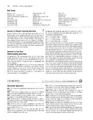15 can be rearranged into the following form: 1E-50 22 24 26 28 30 32 34 end-to-end distance FIG. 1. The self-consistency factor C FR vs the distance Å between the terminus N atom that is fixed and the terminus C atom that is pulled at constant velocity v. Px 0 ,t 0 x 1 ,t 1 ¯ x N ,t N = exp− GPx N ,t 0 x N−1 ,t 1 ¯ x 0 ,t N exp− Wx N ,x N−1 , ...,x 0 . 18 Multiplying the two sides of Eq. 18 with an arbitrary but finite function fWx 0 ,x 1 ,...,x N , integration over coordinates at all times immediately leads to the CFT in the following form: exp− G = fW A→B F /f− W B→A exp− W B→A R . 19 At this point, it is appropriate briefly look into the CFT’s self-consistency. Choosing fW=1, Eq. 19 gives the freeenergy difference through exp−G=1/exp−W B→A R . Choosing fW=e −W , it leads to the well-known JE, exp −G=exp−W A→B F . The self-consistency and thus the validity of the CFT and JE demand that C FR exp− W A→B F exp− W B→A R =1. 20 Equation 20 is a very strong constraint and therefore severely limits the CFT’s applicability. It has been shown 8 that, for near-equilibrium processes, Eq. 20 is simply the linear FDT. For processes that are not near equilibrium; the selfconsistency requirement, Eq. 20, is far from being satisfied. I have done in silico experiments of unfolding titin 1TIT in vacuum. The CHARMM27 force fields are used for the interatomic interactions. NAMD/SMD Ref. 10 is used for the numerical undertakings. I sampled ten unfolding and ten refolding paths to compute the consistency factor C FR defined in Eq. 20. The consistency C FR is plotted in Fig. 1 as a function of the end-to-end distance for two unfolding/refolding speeds. As expected, C FR is closer to 1 for the speed of 0.1 Å/ps than for the speed of 1.0 Å/ps. Even in the case of 0.1 Å/ps, though, C FR is still very far from 1, which means CFT is not self-consistent for these far nonequilibrium processes. Now it is time to examine whether or not the assumption of microscopic reversibility is valid. From the definition of work, we have Author complimentary copy. Redistribution subject to AIP license or copyright, see http://jcp.aip.org/jcp/copyright.jsp
Page 1: THE JOURNAL OF CHEMICAL PHYSICS 129

Nonequilibrium fluctuation-dissipation theorem of ... - LY Chen

Create successful ePaper yourself

Delete template?

Save as template?