Math 2243 Solutions for Fall 2005 Final Exam

Math 2243
Solutions for Fall 2005 Final Exam
!
1) We have a first-order linear differential equation of the form y ’ + P ( x ) y = Q ( x ) ,
in this case a rather simple one with P ( x ) = 3 and Q ( x ) = 5 . To solve an equation
of this sort, we first multiply it through by a function I ( x ) called an “integrating
factor”. The property which determines how this function is chosen is that the left-hand
side of the differential equation takes on a form satisfying the Product Rule, making it
simple to integrate and allowing us to obtain the function y :
I ( x ) y ’ + I ( x ) P ( x ) y = I ( x ) Q ( x ) ! [ I ( x ) y ] ’ = I ( x ) Q ( x )
" I ( x ) y = # I ( x ) Q( x ) dx " y =
I ( x ) Q( x ) dx
For this approach to work, we must have I ’ ( x ) = I ( x ) P ( x ) in our equation, since
the Product Rule gives us I ( x ) y ’ + I ’( x ) y = [ I ( x ) y ] ’ . The integrating factor is
thus specified ! by a separable differential equation of its own, leading to
d I
I ( x )
#
I ( x )
= P( x ) dx " ln I ( x ) = # P( x ) dx " I ( x ) = e
The integrating factor for our equation is then
here, we can proceed to its general solution:
.
# P( x ) dx
.
I ( x ) = e 3 dx " = e 3x . From
e 3x y ’ + 3 e 3x y = 5 e 3x ! [ e 3x y ] ’ = 5 e 3x
!
" e 3x y = # 5 e 3x dx = 5 3 e3x + C " y = 5 3 + C e$3x .
[Note that while the indefinite integral determining the integrating factor does not take
on an “arbitrary constant, the final indefinite integral for the general solution of the
differential ! equation must do so.]
!
2) A frequently-applied technique for analyzing a second-order differential equation is
to create a second variable, say, v = y ’ , which is the derivative of the function to be
solved for. This allows us to transform the single equation into a system of two firstorder
differential equations. In this problem, we thus have
y'' " y y' + 2 y' " y 2 + 5 y = 0 # v = y' , v' " y v + 2 v " y 2 + 5 y = 0
or y' = v , v' = ( y " 2) v + ( y " 5) y .!
!
The derivative of y is zero for any constant value of v , a statement which doesn’t give
us a lot of information about the critical points of this system. However, if v is set to
zero, then the derivative of v becomes zero where the second term of the equation is
!
equal to zero, at y = 0 and y = 5 . (For v ! 0 , the first term can only become zero
at y = 2 , which fails to make the second term equal to zero as well.)

Consequently, the system has two equilibrium points, located at ( 0, 0 ) and
( 5, 0 ) in a v versus y graph. In order to analyze the stability of the system at these
points, we need to evaluate the Jacobian matrix for the system at those positions:
!
y' = f (v, y ) = v , v' = g(v, y ) = ( y " 2) v + ( y " 5) y !
!
! "
# f y ( y 0 , v 0 ) f v ( y 0 , v 0 ) & # 0 1 &
J ( y 0 , v 0 ) = %
( = %
(
$ g y ( y 0 , v 0 ) g v ( y 0 , v 0 ) ' $ v + 2y ) 5 y ) 2 '
( y 0 , v 0 )
.
# 0 1 &
So at ( 0, 0 ) , we have J (0 , 0) = % (!!, corresponding to the
!
$ " 5 " 2 '
linearization y' = v , v' = " 5 y " 2 v! , which has the eigenvalue equation
( –" ) ( #2 – " ) + 5 = " 2 + 2" + 5 = 0 . The eigenvalues are thus
!
!
" = #2 ± 22 # 4 $1 $ 5
2 $ 1
=
#2 ± #16
2
= #1 ± 2i .
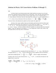
Since these are complex, the flow field circulates around the origin, but the negative real
part indicates that the flow is drawn toward that point [the associated solution
functions ! have the form e "t (cos 2t + sin 2t ) ]. Hence the equilibrium point at the
origin is a stable spiral (also called a “spiral sink”).
!
the flow field in the neighborhood of the origin
(continued)

!
"
At the other equilibrium point, ( 5, 0 ) , we have J (0 , 0) = 0 1 %
$ '!!, which
# 5 3&
corresponds to the linearization [u + 5]' = v , v' = ([u + 5] " 2) v + ([u + 5] " 5)[u + 5]
" u ' = v , v' = 5u + 3v , where we have applied a shifted variable u = y + 5 to make
( 5, 0 ) the center of the flow field. The eigenvalue equation here is ( –" ) ( 3 – " ) # 5
!
= " 2 # 3" # 5 = 0 , giving us the eigenvalues
!
" = #[ #3] ± [ #3]2 # 4 $1 $[ #5]
2 $ 1
= 3 ± 29
2
.
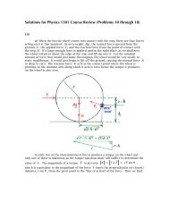
Since "29 > 3 , we have one positive and one negative eigenvalue; this means that the
flow field moves toward ( 5, 0 ) , generally along the direction of the eigenvector for the
negative eigenvalue, ! and away from theat point, generally along the direction of the
eigenvector for the positive eigenvalue (we do not need to find those eigenvectors here).
Eigenvalues of opposite signs thus are the indicators of a “saddle point”.
the flow field in the neighborhood of ( 5, 0 ) ,
shifted to the center of coordinates
The flow field of the complete non-linear system is shown in the graph below.
(continued)

the actual non-linear flow field for the system
!
3) It will be helpful to start by getting a sense of how the given linear transformation in
this Problem works. The transformation T ( v ) “maps” a 3 $ 1 matrix in R 3 into a
2 $ 1 matrix in R 2 , according to T (v ) = 2 2 2
" v
" % 1
%
$ ' "
$ ' v
# 2 3 2 2
&
$ '
= 2v 1 + 2v 2 + 2v 3
%
$
' .
# 2v
# $ v 3 &'
1 + 3v 2 + 2v 3 &
The kernel (or “null space”) of this transformation is the set of 3 x 1 matrices
"
for which T (v ) = 0 = 0 %
$ ' , so it is described by the system of linear equations
# 0
!&
2v 1 + 2v 2 + 2v 3 = 0
!!. If we subtract the first equation from the second either
2v 1 + 3v 2 + 2v 3 = 0
algebraically or by row-reduction of the coefficient matrix for T ( v ) , we find that
!
v 2
= 0 . Inserting this into either of the system equations then leads us to v 1
= #v 3
.
The system of equations cannot be solved any further than this, so this last equation
tells us that there is one “free variable” in the system; we may choose this to be either v 1
or v 3
. If we decide to assign an arbitrary value to v 1
, it is customary to declare that
# 1 &
% (
number to be 1 . This allows us to construct the solution vector
%
0
(!!; but any scalar
$ %"1'(
multiple of this vector will also serve as a solution to our system of equation. Hence, the
) # 1 &
-
+ % (
+
!
kernel of this transformation is the set ker(T )* = * a
%
0
(
, a being any real number.
+
, $ %"1'(
+ .
/
* also called Null ( T ) (continued)
!

Since all of the vectors in the kernel have the same direction vector, they can be
thought of as all falling on a single line in three-dimensional space. The vector subspace
so described is thus one-dimensional, meaning that the dimension of ker ( T ) (also
referred to as “the nullity” of T ) is dim(kernel) = 1 . We have a theorem stating that the
rank of T (or the dimension of the range space of T ) is given by rank ( T ) + dim(kernel)
= n , with n being the dimension of the vector space that T operates within. The
transformation maps vectors in R 3 , so we have rank ( T ) + dim(kernel) = 3 !
rank ( T ) = 3 # 1 = 2 . We can also see this by considering the mapping by T to a
" A %
non-zero vector T (v ) = $ ' , with A and B not both permitted to be zero. We now
# B &
have v 2
= B – A , but still with v 1
= #v 3
. So the solutions of the linear system of
# a &
% (
equations, which constitute the range of T , have the form b = B " A
!
% (!!. Because a and
$ % "a '(
b are not related to one another, these vectors lie in a particular plane in R 3
; hence,
rank( T ) = 2 . (Evidently, not every vector in R 3 is in the range of T ).
!
# 1 1 &
4) The system of two linear differential equations, x' = %
$ "2 4 '
( x + # 1 &
%
$ 3 ( , is
'
non-homongeneous, so we must solve for the solution functions in two parts, one being
# 1 1 &
the “complementary solution”, x C
, to the homogenous system x' = % ( x and
"2 4
!
$ '
the “particular solution”, x P
, which takes the non-homogeneous term into account.
The complementary solution functions are found by first determining the
eigenvalues and corresponding eigenvectors for the coefficient ! matrix in the system. By
1 " # 1
evaluating the determinant
"2
!!, we can set up the eigenvalue equation
4 " #
( 1 – " ) ( 4 – " ) # ( #2 ) = 0 ! " 2 # 5" + 6 = 0 ! ( " # 2 ) ( " – 3 ) = 0 . So the
eigenvalues of the system are " = 2 and " = 3 , which have the corresponding
eigenvectors
" = 2 :
!
$ 1 # 2 1 ' $
&
) &
% #2 4 # 2 ( %
v 1
v 2
'
(
) = $ 0 '
&
% 0 ) * # v 1 + v 2 = 0
( # 2v 1 + 2v 2 = 0 * v 1 = v 2 ,
!
!
so we have one free variable and may chose v 1
= 1 , giving us the
" 1 %
eigenvector $ '!!;!
# 1 &
$ 1 # 3 1 ' $
" = 3 :
!
&
) &
% #2 4 # 3(
%
v 1
v 2
'
(
) = $ 0 '
&
% 0 ) * # 2 v 1 + v 2 = 0
( # 2v 1 + v 2 = 0 * 2 v 1 = v 2 ,
!
leading to the eigenvector
" 1 %
$ '!!.
# 2 &
(continued)
!

The eigenvalues tells us that the exponential solution functions are x 1
x 2
= e 3t , which leads to the complementary solution
= e 2t and
"
x c = x 1%
" 1%
$ ' = c 1 $ ' e 2t " 1 %
+ c
# & # 1
2 $ ' e 3t
& # 2 &
x 2
or
" c 1 e 2t + c 2 e 3t %
$
# c 1 e 2t + 2c 2 e 3t ' .
&
The non-homogeneous term is a column matrix with constant entries, so the trial
functions for the particular solution will also be constants (these would correspond to
an eigenvalue ! of zero, since e 0 · t = 1 , so there is no duplication of terms in the
"
complementary solution). We will then insert x p = A %
$ '!!into our non-homogeneous
# B&
system of differential equations to find
d
dt
" A%
$ ' =
# B&
" 1 1 %"
$
(2 4
!
# &
' A %
$
# B &
' + " 1 %
$
# 3 &
' ) " 0 %
$
# 0 ' =
&
" 1 1 %"
$
# (2 4 &
' A %
$
# B &
' + " 1 % "
$
# 3 ' ) 1 1 %"
$
& # (2 4 &
' A % "
$
# B ' = (1 %
$ ' .
& # (3 &
We may now use whichever method we like for solving a system of linear algebraic
!
equations (substitution, row-reduction, etc.) to calculate that
A = " 1 6 and B = " 5 6 .
Thus, the general solution for our system of differential equations is
" 1%
!
x = x c + x p = c 1 $ ' e 2t " 1 % "
+ c
# 1
2 $ ' e 3t + ( 1 %
$ 6 '
& # 2 & #
$
&
'
( 5 6
or
"
c 1 e 2t + c 2 e 3t ( 1 %
$
6
#
$ c 1 e 2t + 2c 2 e 3t ( 5 '
6 &
'
.
!
d
dt
We can place this into the original system to verify the solution:
#
c 1 e 2t + c 2 e 3t " 1 &
%
6
$
% c 1 e 2t + 2c 2 e 3t " 5 (
6 '
( = # 2c 1 e 2t + 3c 2 e 3t &
%
$ 2c 1 e 2t + 6c 2 e 3t (
'
!
=
# 1 1 &
% (
$ "2 4 '
#
c 1 e 2t + c 2 e 3t " 1 &
%
6
$
% c 1 e 2t + 2c 2 e 3t " 5 (
6 '
( + # 1 &
% (
$ 3 '
!
!
=
=
#
(c 1 e 2t + c 2 e 3t " 1 6 ) + (c 1 e 2t + 2c 2 e 3t " 5 6 ) + 1 &
%
("2) (c 1 e 2t + c 2 e 3t " 1 6 ) + 4 (c 1 e 2t + 2c 2 e 3t " 5 (
$
%
6 ) + 3 '
(
#
(c 1 + c 1 ) e 2t + (c 2 + 2c 2 ) e 3t " 1 " 5 6 6 + 1 &
%
(" 2c 1 + 4 c 1 ) e 2t + (" 2c 2 + 8c 2 ) e 3t + 2 6 " 20 (
$
%
6 + 3 '
( = # 2c 1 e 2t + 3c 2 e 3t &
%
$ 2c 1 e 2t + 6c 2 e 3t ( .! !
'
!

5) To test for the linear independence of three functions on an interval, we evaluate the
f g h
Wronskian determinant
W ( f , g, h ) =
f ' g' h'
f '' g'' h''
; if this determinant is zero
everywhere on the interval, then there is linearly dependence among this set of
functions. For the functions given in this Problem, we find that the Wronskian is
W =
3t + 15
!
3t " 15 te t
3 3 e t + te t = (t + 1)e t
0 0 e t + (t + 1) e t = (t + 2)e t
!
= (t + 2)e t 3t + 15 3t " 15
3 3
= [ (9t + 45) " (9t " 45) ] (t + 2)e t = 90 (t + 2)e t .!
This determinant is zero only at the single value t = #2 , so these three functions are
linearly independent on the real numbers [the interval ( #% , % ) ].
!
The function t is in the span of this set S of functions if there is some linear
combination A f + B g + C h = t , with A , B , and C are real numbers. With
A ( 3t + 15 ) + B ( 3t # 15 ) + C ( t e t ) = t , it is clear that C must be zero, since the
function on the right-hand side has no exponential factor. However, we still require that
( 3A + 3B ) t + ( 15A – 15B ) = t . As there is no constant term on the right-hand side,
we have A = B . It must then be the case that 3A + 3B = 6A = 1
" A = 1 6 = B .
So there does exist a linear combination of the three given functions which can produce
the function t , which means that this function is in the span of the set S .
!
6) For a second-order linear differential equation with constant coefficients,
a y ’’ + b y ’ + c y = 0 , there are two solution functions having a factor e rx . The
constants in the exponents of these functions are the roots of the characteristic
equation ar 2 + br + c = 0 ; if the roots have distinct values r 1
and r 2
, then the
solution functions will simply be e r 1 x
and e r 2 x . The general solution to the
homogenous equation is then the linear combination
y c = c 1 e r 1 x + c 2 e r 2 x .
For our differential equation, y ’’ + 4 y ’ # 9 y = 0 , we have the characteristic
!
equation r 2 + 4r # 9 = 0 with the roots
!
r 1,2 = " 4 ± 4 2 " 4 #1 # (" 9)
2 # 1
= " 4 ± 52
2
= " 2 ± 13 .
The complementary solution is thus y c = c 1 e ( "2 " 13 )x + c 2 e ( "2 + 13 )x ; since the
differential equation is homogeneous, this is the complete general solution.
!
!

!
7) We have a single tank initially containing 10 gallons of pure water. We wish to track
the mass of salt, y ( t ) , found in the tank at later times, given that brine with a
concentration of c in
= 5 lb./gallon* is being poured into this tank at the rate
" dV %
$ ' = 2 gallon/min. and, assuming thorough mixing of the contents of the tank, the
# d t &
in
" dV %
resulting solution is being drained at $ ' = 4 gallon/min. (Since the water in the
# d t &
out
tank is initially pure, we have y ( 0 ) = 0 ) .
!
!
* just go with it, though I’d like to see someone get five pounds of salt to dissolve in one
gallon of water…
!
We will need to write a “mass flow rate” equation describing what is happening
" dy % "
within the tank: generically, this is $ ' = dy % "
$ ' ( dy %
$ ' . The mass of salt
# dt & dt
net
# & dt
in
# &
out
being carried by a solution is given by y = c · V , where c is the salt concentration of
the solution and V is the volume under consideration. Since this is a product of two
" dy % "
quantities, the time derivative ! is properly given by $ ' =
dc % " dV %
$ ' ( V + c ( $ ' . Thus,
# dt & # dt & # dt &
the net rate of change for the mass of salt in the tank is also given by
" dy % "
$ ' = dc %
" dV %
$ ' ( V + c(t ) ( $ ' .
# dt & dt
net
# &
# dt &
net
!
For the brine being sent into the tank, the concentration of salt is constant, so we
" dy % " dV %
write $ ' = c
# dt in ( $ ' . The solution being drained from the tank, however, has
& dt
in
# &
in
the salt concentration found within the tank at any given moment, so c out
= y ( t ) / V ,
with V here being the volume of solution presently in the tank; hence, we write (for the
" dy % " dV %
moment) $ ' = c
# dt out ( $ ' = y(t )
&
dt
out
# &
out
V
( " dV %
$ ' .
# dt &
out
Because the rates at which solution is being added to or removed from the tank
do not match, the volume of liquid in the tank is itself a function of time. We can write
a !“volume flow rate” equation, analogous to the mass flow equation, which is
"
$
#
dV
dt
%
'
&
net
"
= dV %
$ '
# dt &
in
"
( dV %
$ '
# dt &
out
= 2 gal.
min.
( 4 gal.
min.
= ( 2 gal.
min.
.
With an initial volume in the tank V ( 0 ) = 10 gallons, we can easily find the function
describing the volume at later times as V ( t ) = 10 # 2t gallons.
!
We can now develop the complete mass flow rate differential equation which we
will need to solve under the initial conditions given. The rate at which salt is leaving the
" dy %
tank is $ ' = y(t )
# dt &
out
V (t ) ( " dV % y(t )
$ ' =
# dt &
out
10 ) 2t ( 4 . This gives us the mass flow equation
(continued)
!

" dy %
$ '
# dt &
net
"
= dc %
" dV
$ ' ( V (t ) + c(t ) ( $
# dt &
# dt
%
'
&
net
"
= dc %
*"
dV
$ ' ( V (t ) + c(t ) (,
$
# dt &
+ # dt
%
'
&
in
"
) dV %
$ '
# dt &
out
-
/
.
!
"
= dy %
$ '
# dt &
in
"
( dy %
$ '
# dt &
out
" dV
= c in ) $
# dt
%
'
&
in
( y(t )
V (t ) ) " dV %
$ '
# dt &
out
!!.
At this point, we can go one of two ways with this equation. If we choose to
express the differential equation in terms of the mass of salt in the tank, then we need
the equation ! for the net rate of mass flow,
dy
dt
# dV
= c in " %
$ dt
&
(
'
in
) y(t )
V (t ) " # dV &
% (
$ dt '
out
= (5 " 2) )
y(t )
10 ) 2t " 4 ,
!
which is a first-order linear differential equation, but is not separable. We could instead
produce a differential equation for the concentration of salt in the tank,
!
" dc %
*"
dV % "
$ ' ( V (t ) + c(t ) ( $ ' ) dV % - " dV % " dV %
, $ ' / = c
# dt &
+ # dt & dt
in ( $ ' ) c(t ) ( $ ' !
in
# &
out . # dt & # dt &
in
out
!
#
! " dc &
# dV & #
% ( ) V (t ) = [ c
$ dt
in * c(t ) ]) % ( " dc &
% ( ) (10 * 2t ) = [ 5 * c(t ) ]) 2 ,
'
$ dt ' $ dt '
in
which is a separable equation; after solving for c ( t ) , we would then find the mass
function for the salt from y ( t ) = c ( t ) · V ( t ) .
!
The differential equation for mass can be arranged into the form upon which we
can apply an integrating factor by multiplication:
! !
!!
!
!
dy
dt
= (5 " 2) #
y(t )
10 # 2t " 4 $ dy
dt
P( t )dt
I ( x ) = e " = e
" (10 # 2t ) #2 $ dy
dt
"
$
&
%
+
'
(
4
) dt
10 # 2t
% 4 (
' *
& 10 # 2t
14 243
)
P( t )
y = 10 { ; !
Q( t )
= e #2 ln (10 # 2t ) = (10 # 2t ) #2 ;!
%
+ (10 # 2t ) #2 4 (
$ ' * y = 10 (10 # 2t ) #2
& 10 # 2t )
multiplying through by I ( x )
!
" (10 # 2t ) #2 $ dy
dt
+
%
4
(
'
&(10 # 2t ) 3 * y = 10 (10 # 2t ) #2
)
" d
!
dt
* $
1
' .
+ &
%(10 # 2t ) 2 ) y /
,-
( 0 - = 10 (10 # 2t )#2 "
applying the Product Rule
$ 1 '
&
% (10 # 2t ) 2 ) y = 10 1 (10 # 2t ) #2 dt
(
integrating both sides of the equation and
applying the Fundamental Theorem of Calculus
!

$ 1 '
" &
% (10 # 2t ) 2 ) y = 5 (10 # 2t ) #1 + C " y = 5 (10 # 2t ) + C (10 # 2t ) 2 .
(
The initially pure water in the tank requires that y(0) = 5 (10 " 2 # 0) + C (10 " 2 # 0) 2 !
!
!
= 50 + C " 10 2 = 0 # C = $ 1 !!"!!The function for the mass of salt in the tank at
2
time t is therefore
y = 5 (10 " 2t ) " 1 ! 2 (10 " 2t )2 = 10 t " 2 t 2 .
The differential equation for salt concentration in the tank can be separated as
dc
5 " c
=
! 2
10 " 2t dt # dc
$ =
5 " c
dt
$ # " ln 5 " c = " ln 5 " t + C ;
5 " t
since the water in the tank is initially pure, we require
!
!
! !
c(0) = 0 " # ln 5 # 0 = # ln 5 # 0 + C " C = 0!
" # ln 5 # c = # ln 5 # t " 5 # c = 5 # t " c(t ) = t .
!
The function for the mass of salt in the tank is then obtained from y ( t ) = c ( t ) · V ( t )
= t ( 10 # 2t ) = 10 t # 2 t 2 , as we found above.
!
Since the tank is being drained faster than it is being filled, the volume of
solution in the tank will fall to zero in a finite amount of time; in fact, this occurs at
V ( t ) = 10 # 2t = 0 ! t = 5 minutes . From this, we see that the mass of salt in
the tank will also be driven to zero at that time, that is, y ( 5 ) = 0 , as we would
expect. Perhaps surprisingly, the concentration of salt is c ( 5 ) = 5 lb./gallon then.
The interpretation of this result is that just as the tank is about to be emptied
completely, the liquid remaining in the tank is just about entirely from the brine being
pumped into it, so the concentration of salt in the tank approaches the concentration of
the entering brine in the limit as V ( t ) approaches zero.
8) We have a difference of terms in the exponent of the exponential function in the
given differential equation, so it will be helpful to apply the properties of exponents in
dy
order to simplify this expression: = e 3t " y = e 3t # e "y = e 3t
dt
e y .
We can now see from this result that the differential equation is separable, allowing us
to proceed to a general solution:
" e y dy = e 3t dt # e y dy
!
$ = $ e 3t dt # e y = 1 3 e3t + C .
it is convenient at this point to apply the initial condition y ( 0 ) = 0 to find
!
e 0 = 1 3 e3 " 0 + C # 1 = 1 3 "1 + C # C = 2 3 . !
It remains to solve the equation we’ve produced for the specific solution for y ( t ) :
!
" e y = 1 3 e3t + 2 3 # y(t ) = ln $ 2 3 + 1 '
&
% 3 e3t ) .!
(
!

!
9) In order for a set to form a vector space, it must be the case that any linear
combination of vectors in the set must also be a member of that set. The specification
" x %
for the set of two-dimensional vectors $ ' in this Problem is that the product of the
# y &
" a %
components is zero, that is, x y = 0 . The vectors in this set all have the forms $ '
# 0 &
" 0 %
!
or $ ' , where a and b are any real numbers. But the sum of two such vectors is
# b &
" a % "
!
$ ' +
0 % "
$ ' =
a %
$ ' , which generally will have a · b ! 0 . Hence, this set is not closed
# 0 & # b & # b &
under addition and thus cannot form a vector subspace of R 2 .
!
10) We are given the first-order non-homogeneous linear differential equation with an
initial condition, t y ’ # y = t 2 cos t , with y ( & ) = 3 . The equation can be written
in a form for which we can determine an integrating factor (as discussed in Problem 1 ) :
" y' # 1 { t
y = t 1 cos 23 t
P( t ) Q( t )
divide through by t
P( t ) dt
; I (t ) = e$ = e $ # 1 dt t
= e #ln t = 1 t
;
!
" 1 t y' # 1
t y = cos t $ %
'
1 2 & t y (
* ' = cos t $ 1 )
t
multiply through by I ( x )
y = + cos t dt
!
!
" 1 t
y = sin t + C " y = t sin t + C t .
Having found the general solution for the differential equation, we can now apply the
initial condition, in order to determine the specific solution which satisfies it:
Hence, the specific solution to our initial-value problem is
" C = 3 # .
y ( & ) = & sin & + C · & = & · 0 + C · & = 3
#
y = t sin t + % 3 &
( t .
$ " '
!
11) The procedure for solving a system of first-order linear homogeneous differential
equations with constant coefficients is reminiscent of what is done for a single equation;
however, instead of writing a characteristic equation, ! we must instead construct an
eigenvalue equation. We wish to solve the matrix equation Ax = "x , which is
accomplished by finding where the determinant of A – "I = 0 :
7 " # 1 0
"3 3 " # 2
0 0 1 " #
= (1 " # ) 7 " # 1
"3 3 " #
= (1 " # ) [ (7 " # ) (3 " # ) " (" 3) ]
!
= (1 " # ) (# 2 " 10 # + 24 ) = (1 " # ) (# " 4 ) (# " 6) = 0 $ # = 1 , 4 , or 6 .!
(continued)
!

We must next work out the eigenvectors corresponding to each of these
eigenvalues:
" = 1 :
$ 7 # 1 1 0 '
&
)
&
#3 3 # 1 2
)
%&
0 0 1 # 1 ()
$
&
&
%&
x 1
x 2
x 3
'
)
)
()
=
$ 6 1 0 '
& )
&
#3 2 2
)
%&
0 0 0 ()
$
&
&
%&
x 1
x 2
x 3
'
)
)
()
=
$ 0 '
& )
&
0
)
%&
0 ()
*
6 x 1 + x 2 = 0
#3 x 1 + 2x 2 + 2x 3 = 0
one free variable
!
"
# 6 x 1 = x 2
3
2 x 1 # x 2 = x 3
set x 1 = 1
"
$
&
&
&
%
1
# 6
15
2
'
)
)
)
(
$ 2 '
& )
*
&
#12
)
;
%&
15 ()
eliminating fractions
!
!
" = 4 :
$ 7 # 4 1 0 ' $
&
) &
&
#3 3 # 4 2
) &
%&
0 0 1 # 4 ()
%&
"
# 3 x 1 = x 2
set x 1 = 1
x 3 = 0
"
x 1
x 2
x 3
'
)
)
=
()
$ 1 '
& )
&
# 3
)
%&
0 ()
$ 3 1 0 ' $
&
) &
&
#3 #1 2
) &
%&
0 0 # 3 ()
%&
x 1
x 2
x 3
'
)
)
=
()
$ 0 '
& )
&
0
)
%&
0 ()
*
3 x 1 + x 2 = 0
one free variable
x 3 = 0
first and second rows are dependent with x
3
being zero
;
!
!
" = 6 :
$ 7 # 6 1 0 ' $
&
) &
&
#3 3 # 6 2
) &
%&
0 0 1 # 6 ()
%&
"
# x 1 = x 2
set x 1 = 1
x 3 = 0
"
x 1
x 2
x 3
'
)
)
=
()
$ 1 '
& )
&
#1
)
%&
0 ()
$ 1 1 0 ' $
&
) &
&
#3 # 3 2
) &
%&
0 0 # 5 ()
%&
.
x 1
x 2
x 3
'
)
)
=
()
$ 0 '
& )
&
0
)
%&
0 ()
*
x 1 + x 2 = 0
one free variable
x 3 = 0
first and second rows are dependent with x
3
being zero
The solution functions associated with these eigenvalues are e 1·t = e t , e 4t ,
and e!
6t , so the general solution to this homogeneous system is a linear combination of
these exponential functions, dictated by the corresponding eigenvalues; thus,
# 2 & # 1 & # 1 &
% (
x = c 1 %
"12
(
e t % (
+ c 2 %
" 3
(
e 4t % (
+ c 3 %
"1
(
$ % 15 '(
$ % 0 '(
$ % 0 '(
e 6t
or
# 2c 1 e t + c 2 e 4t + c 3 e 6t &
%
"12c 1 e t " 3c 2 e 4t " c 3 e 6t (
%
(
%
$ 15c 1 e t (
'
.
(continued)
!

We can verify that this column matrix of solution functions does in fact satisfy
the given system of differential equations:
!
d
dt
!
!
!
!
!
!
# 2c 1 e t + c 2 e 4 t + c 3 e 6t &
%
"12c 1 e t " 3c 2 e 4t " c 3 e 6t (
%
( =
%
$ 15c 1 e t
(
'
=
# 2c 1 e t + 4 c 2 e 4t + 6c 3 e 6t &
%
"12c 1 e t " 12c 2 e 4t " 6c 3 e 6t (
%
(!
%
$ 15c 1 e t
(
'
# 7 1 0 & # 2c 1 e t + c 2 e 4t + c 3 e 6t &
% ( %
%
"3 3 2
(
"12c 1 e t " 3c 2 e 4t " c 3 e 6t (
%
(!
$ % 0 0 1 '(
%
$ 15c 1 e t
(
'
# (14 " 12)c 1 e t + (7 " 3)c 2 e 4 t + (7 " 1)c 3 e 6t &
%
= ([ " 6 ] " 36 + 30)c 1 e t + ([ " 3] " 9)c 2 e 4 t + ([ " 3] " 3)c 3 e 6t (
%
(!
%
$
15c 1 e t
(
'
=
# 2c 1 e t + 4 c 2 e 4 t + 6c 3 e 6t &
%
"12c 1 e t " 12c 2 e 4t " 6c 3 e 6t (
%
(
%
$ 15c 1 e t
(
'
.! ! !
12) A convenient way to calculate the inverse of a matrix A is to form an augmented
matrix of A combined with the identity matrix I
!
n
of the appropriate dimension, which
then appears as [ A | I n
] , and then perform row-reduction operations to convert the
augmented matrix into [ I n
| A #1 ] . Since our matrix is 3 $ 3 , we place it alongside
I 3
and then carry out the necessary row manipulations:
" 1 1 1 | 1 0 0 %
$
'
$
0 2 1 | 0 1 0
'
# $ 1 0 1 | 0 0 1 &'
(
" 1 1 1 | 1 0 0 %
$
'
0 1 1 2
| 0 1
$
2
0
'
# $ 0 )1 0 | )1 0 1 &'
A I 3
subtract row 1 from row 3 ,
divide row 2 by 2
!
"
$ 1 1 1 | 1 0 0 '
&
)
0 1 1 2
| 0 1
&
2
0 )
0 0 1 2
| #1 1
%
&
2
1 (
)
"
$ 1 1 0 | 3 #1 #2 '
&
)
& 0 1 0 | 1 0 #1 )
0 0 1 2
| #1 1
%
&
2
1 (
)
add row 2 to row 3 subtract row 3 from row 2,
subtract 2 times row 3 from row 1
!
!
"
$ 1 0 0 | 2 #1 #1 '
&
)
&
0 1 0 | 1 0 #1
)
%&
0 0 1 | # 2 1 2 ()
subtract row 2 from row 1,
multiply row 3 by 2
I 3
A # 1
.

We can check to see whether we have found the inverse of A correctly by
multiplying A by A #1 on “either side” to obtain I 3
(one of these will suffice) :
# 2 "1 "1 &
%
(
%
1 0 "1
(
$ % "2 1 2 '(
# 1 1 1&
% (
%
0 2 1
(
$ % 1 0 1'
(
=
# 2 + 0 " 1 2 " 2 + 0 2 " 1 " 1 &
%
(
%
1 + 0 " 1 1 + 0 + 0 1 + 0 " 1
(
$ % "2 + 0 + 2 "2 + 2 + 0 "2 + 1 + 2 '(
=
# 1 0 0 &
% (
%
0 1 0
(
$ % 0 0 1 '(
or
!
" 1 1 1%
$ '
$
0 2 1
'
# $ 1 0 1&
'
" 2 (1 (1 %
$
'
$
1 0 (1
'
# $ (2 1 2 &'
=
" 2 + 1 ( 2 (1 + 0 + 1 (1 ( 1 + 2 %
$
'
$
0 + 2 ( 2 0 + 0 + 1 0 ( 2 + 2
'
# $ 2 + 0 ( 2 (1 + 0 + 1 (1 + 0 + 2 &'
=
" 1 0 0 %
$ '
$
0 1 0
'
# $ 0 0 1 &'
. !
!
G. Ruffa – 7/11