kinematics equations of a class of 4dof parallel wrists

KINEMATICS EQUATIONS OF A CLASS
OF 4DOF PARALLEL WRISTS
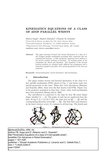
Matteo Zoppi a , Dimiter Zlatanov b , Clément M. Gosselin c
a Università di Genova, via Opera Pia 15A, 16145, Genova, Italia
b Universität Innsbruck, Technikerstr. 13, A-6020, Innsbruck, Austria
c Département de Génie Mécanique, Université Laval, Québec, QC, Canada
zoppi@dimec.unige.it, [zlatanov, gosselin]@gmc.ulaval.ca
Abstract The paper discusses forward and inverse kinematics of a class of 4-
dof 4-legged parallel mechanisms providing three rotational and one
translational freedoms. A fully parametric analytical form solution to
the inverse position problem is provided. All working modes of the
mechanism are shown and discussed. The equations of the forward
position problem are obtained under different leg arrangement and a
numerical example is provided. New special geometries in the class are
proposed.
Keywords: forward kinematics, inverse kinematics, 4dof mechanisms
1. Introduction
The paper studies inverse and forward kinematics of the class of 4-
dof, parallel mechanisms (PMs) shown in Fig. 1, and shows some new
special geometries in the class. When they were introduced (Zlatanov
and Gosselin, 2001), these were the first known 4-dof PMs. Figure 1(a)
is the geometry presented at that time. Later, other 4-dof mechanisms
have been presented, Huang and Li, 2002.
The end-effector is connected to the base by four 5R serial chains
(legs), labelled A, . . .,D. The joints of each leg are numbered from the
base. In leg L (L ∈ {A, B, C, D}), the joint axes are ξ L 1 , . . .,ξ L 5 and the
corresponding direction vectors k L 1 , . . .,kL 5 . The first three axes intersect
in the fixed rotation center, O, common to all four legs. The fourth and
C
D
O
B
A
B
C
O
A
D
D
C
O
B
A
(a)
Figure 1.
(b)
(c)
Mechanisms in the class.

fifth joints are parallel. The platform joint axes, ξ A 5 , . . .,ξ D 5 , are parallel
to the platform plane, π h , which can be chosen arbitrarily among all
planes fixed in the end-effector with the same normal, k. Assuming that
the ξ L 5 are not all parallel, the platform has a full rotational mobility
around O and translates orthogonally to π h (Zlatanov and Gosselin,
2001). The choice of four legs allows to control the PM by actuating
base joints only. The mechanism works with any number of legs greater
than one and part of the results can be extended to the general, m-
legs layout. The extrusion (or heave), h, of the platform (representing
the amount of translation) is the distance between π h and the parallel
0-extrusion plane, π 0 , through O.
2. Geometry
We use: a platform reference frame Pijk (k ⊥ π h ), at the projection,
P, of O on π h ; a rotating frame Oijk; a base frame, Oi b j b k b . The leg L
heave plane, πe L , is through O and orthogonal to ξ L 5 . Points P4 L and P 5
L
are the intersections of πe L with ξ L 4 and ξ L 5 , respectively. The distance
from P4 L to P 5 L is lL 45 ; rL 4 is between P 4 L and O. The constant angle αL 34 ,
spanned by the third leg link, is from ξ L 3 to −→ OP
L
4 (Fig. 2(b)). The angles
of the first two links, αi L i+1 , i = 1, 2, are between kL i and k L i+1 . The set
{l45 L , rL 4 , αL 34 , αL 12 , αL 23 } gives the geometry of leg L standing alone.
How leg L is placed in the mechanism is described by: the distances
r5 L from P 5 L −→
to OP, and h L from π h to ξ L 5 ; the angles θ L between πe L and
Oik; and the tilt, α1 L, and azimuth, βL 1 , angles that place ξL 1 in Oi b j b k b .
The leg can be divided into heave section and spherical section, formed
by the third and fourth, and first two links, respectively. The PM’s heave
and spherical sections are the end-effector with all leg heave sections, and
the base and the leg spherical sections.
A PM is rhombic, if its leg heave sections are two by two equal (l45 M=lN 45 ,
r4 M =rN 4 , αM 34 =αN 34 , {M, N} = {A, C}, {B, D}) and symmetrical, with
πe L coincident (r5 M = r5 N, θM − θ N = π). Also, πe M ≡ πe N , ψ4 M = ψ4
N
(ψ4 L = ∠P 4 LOP L ) and (k M 4 −kN 4 )⊥k. A rectangular PM is rhombic with
πe A ⊥πe B ; a square PM is a rectangular with four identical legs.
Fig. 1 shows two new mechanisms with two nontrivial special geometries.
In 1(b) the platform joints coincide, two by two, along two
skew axes (r5 L = 0 ∀L, hA = h C ≠ h B = h D ); the base joints are coaxial
(α1 L = π/2 ∀L). The end-effector has a straight shape along the axis
through Ok. This geometry can be quite interesting for robotic applications.
In Fig. 1(c) the fifth joints are two by two coincident and form
a cross(r5 L = hL = 0 ∀L). The end-effector has a compact cross shape.

k L 3
n L
45
πh
k L 4r
P 5
L
P 4
L
_ L
k
_
4r
ω L 4
k
P L
P
l 45
L
P 5
L
πh
α 34
L
ψ L
4
P 4
L
r 5
L
P L
h h L
ε L =1
ε L =-1
P L
k L 4
(a)
χ L
O
(b)
r L
4
r L
int
r45
L
O
πO
(c)
O
Figure 2.
Heave section of leg L: vectors (a); parameters (b); working modes (c).
3. Inverse Kinematics
The end-effector pose is given by the extrusion, h, and the platform
orientation matrix, R. The aim is to compute the PM’s entire configuration.
First, we solve the heave section, then the spherical section.
Unless noted otherwise, vectors are given in the end-effector frame.
Heave-section. Consider the leg L heave section. Point P L is the
projection of O on the plane through ξ L 5 parallel to π h (Fig. 2); the
quadrilateral OP L P5 LP 4 L is a virtual 1-dof mechanism with parameter
h. We obtain k L 3 in the reference frame O(kL 4 ×k)kL 4 k, and then in Oijk.
First, we get c L 4 = cos ψL 4 , sL 4 = sinψL 4 . We have
2r L 4 H L c L 4 + 2r L 4 r L 5 s L 4 − H L2 − N L = 0 (1)
where H L = h+ h L , N L = r5
L 2 + r
L2 4 − l
L 2
45 . The solutions of (1) are:
[
c
L
4 s L 4
[
] T =(2r
L
4 (H L2 +r5
L 2
))
−1 H L −r5
L ] [
r5
L H L H L2 +N L ε L Cε
L
] T
(2)
where ε L = ±1 distinguishes between the two feasible working modes of
the quadrilateral OP L P5 LP 4 L (Fig. 2), and:
√
Cε L = −(H L2 − m L 45 )(HL2 − M45 L ) (3)
with M L 45 =(rL 4 + lL 45 )2 − r L 5
2 and m
L
45 =(r L 4 − lL 45 )2 − r L 5
2 .
The quadrangle takes symmetric configurations for positive and negative
values of h. Consider h ≥ 0. At maximal extrusion, P L 5 , P L 4 and O
are collinear and H L = (M L 45 )1 2. At minimal extrusion (if allowed by the
geometry of the whole mechanism), P L 5 , P L 4 and O are collinear, with P L 5
between P L 4 and O; HL = (m L 45 )1 2. (These are transition configurations

C
A
C
A
D
B
D
B
D
B
D
B
A
C
BD
(a) ε A = +1
(b) ε A = −1
(c) δ A = +1
(d) δ A = −1
Figure 3. Working modes of the heave section ((a) and (b)) and of the spherical
section ((c) and (d)) of leg A.
between the two working modes of the quadrilateral.) It is clear from
(3) that for Cε L to be real, it is necessary that m L 45 ≤ HL2 ≤ M45 L .
To obtain k L 4 in Pijk, we rotate j about k at θL , k L 4 = R z(θ L )j.
Vector k L 4r is computed analogously:
k L 4r = R z (θ L ) [ s L 4 0 cL 4
] T
(4)
Now an α34 L rotation about kL 4 ⊥πL e gets k L 3 = R e(α34 L )R z(θ L ) [ s L 4 0 ] T.
cL 4
The four ε L , one for each leg, distinguish between four different working
modes of the heave section of the mechanism. Fig. 3 shows the two
working modes of the heave section of one leg.
We compute the components of n L 45 along kL 4r and k⊥L 4r and add them:
n L 45 = R z(θ L )
2 l L 45 rL 4
(
)
ε L Cε L k L 4r + (l45
L 2
+r
L2 4 −r
L2 5 −H
L 2 ) k ⊥L
4r
(5)
where k L 4r
is provided by (4), and k⊥L 4r = k L 4 ×kL 4r .
Spherical section. The poses of the first and second links of leg
L depend both on R and h through the direction vectors k L 1 and kL 3 .
Vector k L 3 is a result of the inverse kinematics of the heave section, while
vector k L 1 is easily obtained by a change of reference frame: kL 1 = RkL 1 b .
It remains to compute vector k L 2 . The axis ξL 2 of the second joint lies
at the intersection of two right circular cones with vertex, axes and halfangle
O,ξ L 1 , α12 L and O,ξL 3 , α23 L , respectively. For ξL 2 to lie on both cones,
k L 2 must satisfy kL 2 · kL 1 = cL 12 and kL 2 · kL 3 = cL 23 , where cL ij = cos αL ij .
Then, k L 2 is obtained as a linear combination of kL 1 , kL 3 and kL 1 ×kL 3 ,
k L 2 = (1 − (k L 1·k L 3 ) 2 ) −1 [ k L 1 kL 3 kL 1 ×kL 3
] [
t
L
1 t L 2 tL 3
] T
(6)
The coefficients are: t L 1 =cL 12 −cL 23 kL 1·kL 3 , tL 2 =cL 23 −cL 12 kL 1·kL 3 , tL 3 =δL C L δ ,
C L δ = √−(k L 1·kL 3 − mL AB )(kL 1·kL 3 − ML AB ) (7)

with m L AB = cL 12 cL 23 −∣ ∣
∣s L 12 sL 23
∣, MAB L = cL 12 cL 23 +∣ ∣
∣s L 12 sL 23
∣, s L ij = sin αL ij . The
boolean parameter δ L =±1 distinguishes between the two working modes
of the spherical section of the leg (Fig. 3).
The rotation angles of the actuated (base) joints, the solution of the
inverse kinematics problem, are easily computed from the four k L 2 .
A leg configuration is feasible (Cδ L in (7) is real) iff ∣ ∣α 12 L − αL ∣
23 ≤
α13 L ≤ ∣ ∣α 12 L + ∣
αL 23
∣, where α13 L = ∠(ξL 1 , ξ L 3 ), i.e. m L AB ≤ kL1·kL 3 ≤ ML AB .
An expressions for the unit-length vector n L 23 , orthogonal to the plane
π23 L defined by ξL 2 and ξ L 3 is:
n L 23 = ∣ ∣s L ∣ −1 (
23 −t
L
3 k L 1 + t L 3 k L 1·k L 3 k L 3 + t L 1 k L 1×k L )
3
Things simplify if c L 12 = cL 23 = 0: (7) becomes CL δ = √1−(k L 1·kL 3 )2 ,
k L 2 ‖ kL 1 ×kL 3 (tL 1 =tL 2 =0) and T L 3 =0.
4. Forward Kinematics
The four k L 2 are given and the pose, (h,R), is unknown.
In the general case, to write a system of equations for the forward
kinematics is quite complicated; a general discussion can be found in Zlatanov
and Gosselin, 2001. Here, we consider rhombic PMs with α34 L = 0,
h L = 0, ∀L. Even for this case, writing a reasonable system of equations
is not obvious. Using, as is usual, h and some rotation parameters as
variables, results in very complex formulations. We have succeeded in
deriving relatively simple equations, however, an analytical form solution
is not known. Such systems can be solved numerically (see Saaty,
1981). We provide an even simpler system of equations for the square
mechanisms. An analytical form solution in this case may be achievable
for particular geometries (see Salmon, 1859, Gohberg et al., 1982),
however, this remains an open problem.
To get four simpler equations, we use as intermediate unknowns the
angles θ2 L (sL 2 = sinθL 2 , cL 2 = cos θL 2 ) of the second joints of the legs,
rather than h and three rotation parameters for R. In leg L, θ2 L is the
angle about k L 2 from πL 12 to πL 23 . Since ξL 3 lies on the cone with axis ξ L 2
and half angle α23 L , an expression of kL 3 as a function of θL 2 is:
(8)
k L 3 (θ L 2 ) = a L c c L 2 + b L c s L 2 + g L c (9)
where a L c = s L 23 kL 1 ×kL 2 , bL c = s L 23
(
c
L
12 k L 2 − ) kL 1 , g
L
c = c L 23 kL 2 .
Rhombic mechanisms. Two equations state that the right, rectangular
pyramid with base edges along ξ L 3 has equal opposite faces, i.e.,

(a) (b) (c) (d)
(e) (f) (g) (h)
fig. θ
2
A θ
2
B θ
2
C θ
2
D
a .0221 .3947 .3535 6.1686
b .5082 1.0353 .8155 .1905
c 1.3246 2.0550 .7475 6.0834
d 2.7094 .0067 5.5956 2.4968
e 2.9029 3.4042 3.7732 3.3844
f 3.1853 3.8419 4.4627 3.9232
g 3.1513 3.8820 4.7720 4.1761
h 4.8807 4.8715 4.6196 4.6091
i 5.5429 2.2388 3.1101 6.2231
(i)
(l)
⎡
⎤
.7846 −.552.2823
l 5.6334 5.2362 3.2778 3.4593
R= ⎣ .552 .8292.0873⎦, h/l 45 =1.04, ε L =δ L =1 ∀L; r 4 /l 45 =.8, β 1 =α 43 =0, α 12 =1.0472, α 23 =.6283
−.2823.0873.9553
Figure 4. Example of solutions for the forward kinematics of a square mechanism.
To improve visibility, base pyramids are represented wire-frame.
∠ξ A 3 ξ B 3 = ∠ξ C 3 ξ D 3 and ∠ξ A 3 ξ D 3 = ∠ξ C 3 ξ B 3 :
k A 3 · k B 3 − k C 3 · k D 3 = 0 (10)
k A 3 · k D 3 − k C 3 · k B 3 = 0 (11)
The third equation describes the angle, θ B −θ A , between πe A and πe B :
(
k
A
3 − k C ) (
3 · k
B
3 − k D )
3 = cos(θ B −θ A ) (12)
By developing Eq. (12), simplifying and substituting in Eqs. (10) and
(11), we obtain the following second degree equations in s L 2 and cL 2 :
k A 3 (θ A 2 ) · k B 3 (θ B 2 ) − k B 3 (θ B 2 ) · k C 3 (θ C 2 ) = cos(θ B −θ A )/2 (13)
k C 3 (θ C 2 ) · k D 3 (θ D 2 ) − k B 3 (θ B 2 ) · k C 3 (θ C 2 ) = cos(θ B −θ A )/2 (14)
k A 3 (θ A 2 ) · k B 3 (θ B 2 ) − k A 3 (θ A 2 ) · k D 3 (θ D 2 ) = cos(θ B −θ A )/2 (15)
and, by means of (9), we write them as three quadratic forms:
X T Q i X = cos(θ B −θ A )/2 i = 1, 2, 3 (16)
where X T = [ s A 2 sB 2 s C 2 sD 2 c A 2 cB 2 c C 2 cD 2 1 ] .

Finally, we express that ψ4 A and ψB 4 satisfy (1) for the same value
of h. We solve (1) for h; since α34 L = 0 and hL = 0, we obtain: h =
r4 LcL 4 + εL (r4
L 2 c
L2 4 −N L +2r4 LrL 5 sL 4
2. )1 Thus, the fourth equation is:
√
r4c A A 4−r4c B B 4 =ε
√r B 4
B 2 c
B2 4 −N B +2r4 BrB 5 sB 4 −εA r4
A 2 c
A2 4 −N A +2r4 ArA 5 sA 4 (17)
After squaring twice, Eq. (17) becomes a second degree equation in
s L 4 , cL 4 . Since the PM is rhombic, kM 3 · k N 3 = cos(2ψ4 M ), {M, N} =
{A, C}, {B, D}. Therefore, c M 2
4 = (1 +k
M
3 ·k N 3 )/2 and sM 2
4 = (1 −k
M
3 ·
k N 3 )/2. Eq. (9) allows to obtain kM 3 · kN 3 as a function of θL 2 .
Eqs. (16–17) are the final system of four equations for the forward
kinematics of rhombic PMs.
Square mechanisms. For square PMs, θ A −θ B =π/2 and Eqs. (16)
are homogeneous. Eq. (17) becomes k A 3 ·kC 3 −kB 3 ·kD 3 = 0, stating that
ψ4 A = ψB 4 . From Eq. (9), we write this fourth equation as a quadratic
form X T Q 4 X = 0. So, the forward kinematics of the square mechanisms
is expressed by a system of four second degree, homogeneous equations
X T Q i X = 0, i = 1, 2, 3, 4. The matrices Q i are given in the Appendix.
Fig. 4 shows a numerical example for a square, cross-platform geometry.
This is the problem of placing a “double-compass” tetrapod on four
circles of a sphere. The system of the forward kinematics equations is:
⎧
⎪⎨
⎪⎩
−0.1907s A 2 cB 2 −0.2892cA 2 −0.377sA 2 +0.32cB 2 +0.8910sB 2 −0.0489 +0.2573cA 2 cB 2 −0.0948cA 2 sB 2 +
+0.0894s A 2 sB 2 −0.0981cC 2 −0.4620sC 2 +0.0567cB 2 sC 2 +0.0934sB 2 cC 2 −0.3249cB 2 cC 2 −0.0589sB 2 sC 2
−0.1739c C 2 −0.9313sC 2 +0.0368sC 2 sD 2 −0.0586−0.042sC 2 cD 2 +0.4506sB 2 +0.2515cD 2 +0.4034sD 2 +
−0.1792c C 2 sD 2 +0.1417cB 2 +0.2902cC 2 cD 2 +0.0567cB 2 sC 2 +0.0934sB 2 cC 2 −0.3249cB 2 cC 2 −0.0589sB 2 sC 2
−0.1907s A 2 cB 2 −0.5963cA 2 −0.73sA 2 +0.1782cB 2 +0.4404sB 2 +0.1436+0.2573cA 2 cB 2 −0.0948cA 2 sB 2 +
+0.0894s A 2 sB 2 +0.2114cD 2 +0.4174sD 2 −0.2143cA 2 cD 2 +0.1538cA 2 sD 2 +0.2232sA 2 cD 2 −0.061sA 2 sD 2
−0.22s A 2 sC 2 −0.26sA 2 cC 2 −0.263cA 2 sC 2 +0.224cA 2 cC 2 +0.223sD 2 sB 2 −0.082sA 2 +0.259cD 2 sB 2 +0.065sC 2 +
−0.016c A 2 +0.0027+0.0525cC 2 +0.262sD 2 cB 2 −0.225cD 2 cB 2 −0.045sD 2 −0.002cB 2 +0.071sB 2 −0.055cD 2
Geometry and configuration parameters are reported in the figure.
We have identified the same ten solutions with several different numeric
procedures, yet, so far, there is no proof that others do not exist.
5. Conclusions
The paper provides an analytical form solution of the inverse kinematics
of a general class of 4-dof PMs. It also presents a relatively simple
formulation of the forward kinematics of an interesting mechanism
subclass, including some new PMs with special geometries. The proposed
mathematical models are fully parametric and free of mathematic
singularities, i.e., valid in all configurations. The obtained equations
are a natural starting point for any further research on this mechanism

class, such as workspace analysis or force transmission, as well for the
design and any practical application of this architecture. Challenging
open problems, related to the solution of the direct kinematics and the
evaluation of the number of possible solutions, remain.
References
Gohberg, T., Lancaster, P., Rodman, L. (1982), Matrix Polynomials, New York, Academic
Press;
Huang, Z., Li, Q.C. (2002), On the Type Synthesis of Lower-Mobility Parallel Manipulators,
Proc. of the workshop Fundamental Issues and Future Research Directions
for Parallel Mechanisms and Manipulators, Québec City, Québec, Canada;
Saaty, T. L. (1981), Modern Non-linear Equations, New York (1967), Dover (1981),
McGraw-Hill;
Salmon, G. (1859), Introductory to the Modern Higher Algebra, Dublin, Hodges,
Smith, and co.;
Zlatanov, D., Gosselin, C. (2001), A family of new parallel architectures with four
degrees of freedom, In F.C. Park C.C. and Iurascu, editor, Computational Kinematics,
pp.57-66, Mai 2001.
Appendix
⎡
0 b B c ·bA c 0 −bD c ·bA c 0 a B c·bA c 0 −aD c ·bA c bAc·gB c − bAc·gD ⎤
c
0 0 0 0 a A c·bB c 0 0 0 b B c ·gA c
0 0 0 0 0 0 0 0 0
0 0 0 0 −a A c·bD c
0 0 0 −b D c ·gA c
Q 1 =
0 0 0 0 0 a B c·aA c 0 −aD c ·aA c aA c·gB c − aA c·gD c
0 0 0 0 0 0 0 0 a B c·gA c
0 0 0 0 0 0 0 0 0
⎢
⎣ 0 0 0 0 0 0 0 0 −a D c ·gA ⎥
⎦
c
0 0 0 0 0 0 0 0 g
c B ·gA c −gD c ·gA c
⎡
0 b B c ·bA c
0 0 0 a B c ·bA c
0 0 b A c·gB ⎤
c
0 0 −b C c·bB c 0 aA c·bB c
0 −a C c·bB c 0 bB c ·gA c −bB c ·gC c
0 0 0 0 0 −a B c·bC c
0 0 −b C c·gB c
0 0 0 0 0 0 0 0 0
Q 2 =
0 0 0 0 0 a B c·aA c
0 0 a A c·gB c
0 0 0 0 0 0 −a C c·aB c 0 aB c·gA c −aB c ·gC c
⎢ 0 0 0 0 0 0 0 0 −a C
⎣
c·gB c ⎥
0 0 0 0 0 0 0 0 0 ⎦
0 0 0 0 0 0 0 0 g
c B ·gA c −gC c ·gB c
⎡ 0 0 0 0 0 0 0 0 0 ⎤
0 0 b C c·bB c 0 0 0 a C c·bB c 0 b B c ·gC c
0 0 0 −b D c ·bC c 0 aBc·bC c 0 −a D c ·bC c bCc·gB c −bCc·gD c
0 0 0 0 0 0 −a C c·bD c
0 −b D c ·gC c
Q 3 =
0 0 0 0 0 0 0 0 0
0 0 0 0 0 0 a C c·aB c 0 a B c·gC c
0 0 0 0 0 0 0 −a
⎢
D c ·aC c aCc·gB c −aCc·gD c
⎣ 0 0 0 0 0 0 0 0 −a D c ·gC ⎥
⎦
c
0 0 0 0 0 0 0 0 gc C ·gB c −gD c ·gC c
⎡
0 0 b C c·bA c 0 0 0 a C c·bA c 0 b A c·gC ⎤
c
0 0 0 −b D c ·bB c 0 0 0 −a D c ·bB c −b B c ·gD c
0 0 0 0 a A c·bC c
0 0 0 b C c·gA c
0 0 0 0 0 −a B c·bD c
0 0 −b D c ·gB c
Q 4 =
0 0 0 0 0 0 a C c·aA c
0 a A c·gC c
0 0 0 0 0 0 0 −a D c ·aB c
−a B c·gD c
0 0 0 0 0 0 0 0 a
⎢
C c·gA c
⎣ 0 0 0 0 0 0 0 0 −a D c ·gB ⎥
⎦
c
0 0 0 0 0 0 0 0 g c·gC A c −gB c ·gD c