Microeconometrics: Homework 1

Microeconometrics: Homework 1
2010
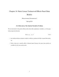
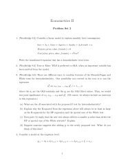
1. Problem 5.1. In this problem you are to establish the algebraic equivalence between
2SLS and OLS estimation of an equation containing an additional regressor. Although
the result is completely general, for simplicity consider a model with a single (suspected)
endogenous variable:
y 1 = z 1 δ 1 + α 1 y 2 + u 1
y 2 = zπ 2 + v 2
For notational clarity, we use y 2 as the suspected endogenous variable and z as the vector
of all exogenous variables. The second equation is the reduced form for y 2 . Assume that
z has at least one more element than z 1 .
We know that one estimator of (δ 1 , α 1 ) is the 2SLS estimator using instruments x.
Consider an alternative estimator of (δ 1 , α 1 ): (a) estimate the reduced form by OLS,
and save the residuals ˆv 2 ; (b) estimate the following equation by OLS:
y 1 = z 1 δ 1 + α 1 y 2 + ρ 1ˆv 2 + error (5.52)
Show that the OLS estimates of δ 1 and α 1 from this regression are identical to the
2SLS estimators. [Hint: Use the partitioned regression algebra of OLS. In particular, if
ŷ = x 1 ˆβ1 + x 2 ˆβ2 is an OLS regression, ˆβ 1 can be obtained by first regressing x 1 on x 2 ,
getting the residuals, say ẍ 1 , and then regressing y on ẍ 1 ; see, for example, Davidson
and MacKinnon (1993, Section 1.4).
You must also use the fact that z 1 and ˆν 2 are
orthogonal in the sample.]
1

Sol: Define x 1 ≡ (z 1 , y 2 ) and x 1 ≡ ˆv 2 , and let ˆβ ≡ ( ˆβ ′ 1 , ˆρ 1) ′ be OLS estimator from
(5.52), where ˆβ 1 = (ˆδ ′ 1 , ˆα 1) ′ . Using the hint, ˆβ1 can also be obtained by partitioned
regression:
(i) Regress x 1 onto ˆv 2 and save the residuals, say ẍ 1 .
(ii) Regress y 1 onto ẍ 1 .
But when we regress z 1 onto ˆv 2 , the residuals are just z 1 since ˆv 2 is orthogonal in sample
to z. (More precisely, ∑ N
i=1 z′ i1ˆv i2 = 0.) Further, because we can write y 2 = ŷ 2 + ˆv 2 ,
where ŷ 2 and ˆv 2 are orthogonal in sample, the residuals from regressing y 2 onto ˆv 2 are
simply the first stage fitted values, ŷ 2 . In other words, ẍ 1 = (z 1 , ŷ 2 ). But the 2SLS
estimator of β 1 is obtained exactly from the OLS regression y 1 on z 1 , ŷ 2 .
2. Problem 5.5. One occasionally sees the following reasoning used in applied work for
choosing instrumental variables in the context of omitted variables. The model is
y 1 = z 1 δ 1 + α 1 y 2 + γq + a 1
where q is the omitted factor. We assume that a 1 satisfies the structural error assumption
E(a 1 |z 1 , y 2 , q) = 0, that z 1 is exogenous in the sense that E(q|z 1 ) = 0, but that y 2 and
q may be correlated. Let z 2 be a vector of instrumental variable candidates for y 2 .
Suppose it is known that z 2 appears in the linear projection of y 2 onto (z 1 , z 2 ), and so
the requirement that z 2 be partially correlated with y 2 is satisfied. Also, we are willing
to assume that z 2 is redundant in the structural equation, so that a 1 is uncorrelated
with z 2 . What we are unsure of is whether z 2 is correlated with the omitted variable q,
in which case z 2 would not contain valid IVs.
To test whether z 2 is in fact uncorrelated with q, it has been suggested to use OLS on
the equation
y 1 = z 1 δ 1 + α 1 y 2 + z 2 ψ 1 + u 1 (5.55)
where u 1 = γq + a 1 , and test H 0 : ψ 1 = 0. Why does this method not work
Sol: Under the null hypothesis that q and z 2 are uncorrelated, z 1 and z 2 are exoge-
2

nous in (5.55) because each is uncorrelated with u 1 , and so the regression of y 1 on
z 1 , y 2 , z 2 does not produce a consistent estimator of 0 on z 2 even when E(z 2 ′ q) = 0. We
could find that ˆψ 1 from this regression is statistically different from zero even when q
and z 2 are uncorrelated–in which case we could incorrectly conclude that z 2 is not a valid
IV candidate. Or, we might fail to reject H 0 : ψ 1 = 0 when z 2 and q are correlated–in
which case we incorrectly conclude that the elements in z 2 are valid as instruments.
The point of this exercise is that one cannot simply add instrumental variable candidates
in the structural equation and then test for significance of these variables using OLS.
This is the sense in which identification cannot be tested. With a single endogenous
variable, we must take a stand that at least one element of z 2 is uncorrelated with q.
3. Problem 10.3. For T = 2 consider the standard unobserved effects model
y it = x it β + c i + u it , t = 1, 2
Let ˆβ F E and ˆβ F D denote the fixed effects and first difference estimators, respectively.
a. Show that the FE and FD estimates are numerically identical.
b. Show that the error variance estimates from the FE and FD methods are numerically
identical.
Sol:
a. Let ¯x i = (x i1 + x i2 )/2, ȳ i = (y i1 + y i2 )/2, ẍ i1 = x i1 − ¯x i , ẍ i2 = x i2 − ¯x i , and similarly
for ÿ i1 and ÿ i2 . For T = 2 the fixed effects estimator can be written as
[
∑ N ] −1 [
∑ N ]
ˆβ F E = (ẍ ′ i1ẍ i1 + ẍ ′ i2ẍ i2 ) (ẍ ′ i1ÿ i1 + ẍ ′ i2ÿ i2 )
Now, by simple algebra,
i=1
i=1
ẍ i1 = (x i1 − x i2 )/2 = −∆x i /2
ẍ i2 = (x i2 − x i1 )/2 = ∆x i /2
ÿ i1 = (y i1 − y i2 )/2 = −∆y i /2
ÿ i2 = (y i2 − y i1 )/2 = ∆y i /2
3

Therefore,
ẍ ′ i1ẍ i1 + ẍ ′ i2ẍ i2 = ∆x ′ i∆x i /4 + ∆x ′ i∆x i /4 = ∆x ′ i∆x i /2
ẍ ′ i1ÿ i1 + ẍ ′ i2ÿ i2 = ∆x ′ i∆y i /4 + ∆x ′ i∆y i /4 = ∆x ′ i∆y i /2
and so
[
∑ N
ˆβ F E =
i=1
] −1 [
∑ N
∆x ′ i∆x i /2
i=1
]
∆x ′ i∆y i /2
[
∑ N ] −1 [
∑ N ]
= ∆x ′ i∆x i ∆x ′ i∆y i = ˆβ F D .
i=1
b. Let û i1 = ÿ i1 − ẍ i1 ˆβF E and û i2 = ÿ i2 − ẍ i2 ˆβF E be the fixed effects residuals for
the two time periods for cross section observation i. Since ˆβ F E = ˆβ F D , and using the
representations in (4.1 ′ ), we have
i=1
û i1 = −∆y i /2 − (−∆x i /2) ˆβ F D = −(∆y i − ∆x i ˆβF D )/2 ≡ −ê i /2
û i2 = ∆y i /2 − (∆x i /2) ˆβ F D = (∆y i − ∆x i ˆβF D )/2 ≡ ê i /2
where ê i ≡ ∆y i − ∆x i ˆβF D are the first difference residuals, i = 1, 2, . . . , N.
Therefore,
N∑
N∑
(û 2 i1 + û 2 i2) = (1/2)
i=1
i=1
This shows that the sum of squared residuals from the fixed effects regression is exactly
ê 2 i
one have the sum of squared residuals from the first difference regression.
Since we
know the variance estimate for fixed effects is the SSR divided by N − K(when T = 2),
and the variance estimate for first difference is the SSR divided by N − K, the error
variance from fixed effects is always half the size as the error variance for first difference
estimation, that is, ˆσ u 2 = ˆσ e/2 2 (contrary to what the problem asks you so show). What I
wanted you to show is that the variance matrix estimates of ˆβ F E and ˆβ F D are identical.
4

This is easy since the variance matrix estimate for fixed effects is
ˆσ 2 u
[
∑ N −1 [
∑ N −1 [
∑ N ] −1
(ẍ ′ i1ẍ i1 + ẍ ′ i2ẍ i2 )]
= (ˆσ e/2)
2 ∆x ′ i∆x i /2]
= ˆσ e
2 ∆x ′ i∆x i ,
i=1
i=1
i=1
which is the variance matrix estimator for first difference. Thus, the standard errors,
and in fact all other test statistics (F statistics) will be numerically identical using the
two approaches.
4. Problem 10.5. Assume that Assumptions RE.1 and RE.3a hold, but V ar(c i |x i ) ≠
V ar(c i ).
a. Describe the general nature of E(v i v i ′ |x i).
b. What are the asymptotic properties of the random effects estimator and the associated
test statistics How should the random effects statistics be modified
Sol:
a. Write v i v i ′ = c2 i j T j
T ′ + u iu ′ i + j T (c i u ′ i ) + (c iu i )j
T ′ ). Under RE.1, E(u i|x i , c i ) = 0, which
implies that E[(c i u ′ i )|x i] = 0 by iterated expectations.
Under RE.3a, E(u i u ′ i |x i, c i ) = σuI 2 T , which implies that E(u i u ′ i |x i) = σuI 2 T (again, by
iterated expectations). Therefore,
E(v i v ′ i|x i ) = E(c 2 i |x i )j T j ′ T + E(u i u ′ i|x i ) = h(x i )j T j ′ T + σ 2 uI T ,
where h(x i ) ≡ V ar(c i |x i ) = E(c 2 i |x i)(by RE.1b). This shows that the conditional variance
matrix of v i given x i has the same covariance for all t ≠ s, h(x i ), and the same
variance for all t, h(x i ) + σu. 2 Therefore, while the variances and covariances depend on
x i in general, they do not depend on time separately.
b. The RE estimator is still consistent and √ N−asymptotically normal without assumption
RE.3b, but the usual random effects variance estimator of ˆβ RE is no longer
valid because E(v i v i ′ |x i) does not have the form (10.30)(because it depends on x i ). The
robust variance matrix estimator given in (7.49) should be used in obtaining standard
errors or Wald statistics.
5