Fine Scale Meteorology & Air Quality Models - School of Architecture ...
Fine Scale Meteorology & Air Quality Models - School of Architecture ...
Fine Scale Meteorology & Air Quality Models - School of Architecture ...

You also want an ePaper? Increase the reach of your titles
YUMPU automatically turns print PDFs into web optimized ePapers that Google loves.
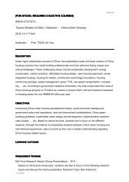
ASI2_Lecture 3_7/12/2011<br />
Croucher Advanced Study Institute 2011<br />
Urban Climatology for Tropical & Sub-tropical Regions<br />
<strong>Fine</strong> <strong>Scale</strong> <strong>Meteorology</strong> & <strong>Air</strong> <strong>Quality</strong> <strong>Models</strong><br />
Urban Forecasting, planning and assessment tools<br />
Jason Ching<br />
Senior Research Fellow, UNC<br />
Institute for the Environment,<br />
Chapel Hill, North Carolina, USA<br />
URBAN AIR POLLUTION<br />
Lecturer’s Photo<br />
ASI 2: URBAN CLIMATE AND AIR POLLUTION <strong>School</strong> <strong>of</strong> <strong>Architecture</strong>, The Chinese University <strong>of</strong> Hong Kong, Hong Kong, 7-8 Dec 2011<br />
Introduction and Background:<br />
Presentation Outline<br />
• Part 1: Introduction and Context<br />
• Part 2: Mesoscale Modeling<br />
– Part 2a: Mesoscale RANS-Urban canopy-based modeling<br />
– Part 2b: Urban canopy descriptions and data<br />
– Part 2c: <strong>Fine</strong> scale mesoscale modeling issues<br />
• Part 3: <strong>Air</strong> <strong>Quality</strong> Modeling: Framework for characterizing<br />
(AQ) sub-grid features<br />
ASI 2: URBAN CLIMATE AND AIR POLLUTION <strong>School</strong> <strong>of</strong> <strong>Architecture</strong>, The Chinese University <strong>of</strong> Hong Kong, Hong Kong, 7-8 Dec 2011<br />
1
ASI2_Lecture 3_7/12/2011<br />
Part 1: Introduction: Multi-scale modeling<br />
Modeling Tools<br />
• Meteorological modeling<br />
• <strong>Air</strong> quality modeling<br />
• Sub-grid context<br />
• Urban modeling<br />
• Canopy, in-canyon modeling<br />
• LES<br />
• CFD<br />
• Local <strong>Scale</strong>-Hybrid modeling<br />
Modeling System Development<br />
•Meteorological Model Developments:<br />
– Hurricane Model-> MM5-> WRF-> MPAS<br />
Multi-scale WRF System<br />
•General Framework<br />
•PBL Formulations<br />
•TKE vs Non-TKE schemes<br />
•Land-surface models<br />
•Urbanization in WRF<br />
•UHI Sensitivity studies<br />
•<strong>Air</strong> <strong>Quality</strong> Model Developments<br />
– Dispersion models-> photochemical grid models<br />
-> Acid Deposition model -> Community<br />
Multiscale One-Atmosphere AQ/Deposition<br />
model<br />
•Climate Model Developments<br />
– GCMs-> Community Climate models-><br />
Community Earth systems model<br />
ASI 2: URBAN CLIMATE AND AIR POLLUTION <strong>School</strong> <strong>of</strong> <strong>Architecture</strong>, The Chinese University <strong>of</strong> Hong Kong, Hong Kong, 7-8 Dec 2011<br />
Common Community<br />
Model Design Features<br />
Examples:<br />
WRF (Meteorological)<br />
CMAQ (<strong>Air</strong> <strong>Quality</strong>)<br />
Preprocessors -> Core -> Postprocessors<br />
Maintenance, Version Controls<br />
Open System<br />
Open Source,<br />
Dynamic Development Framework<br />
User Friendly<br />
Community Support Infrastructure<br />
Multiscale: Gridding/Nesting capabilities<br />
User Setups & Controls<br />
Science evolves; Module options grows<br />
Complementary Documentation<br />
<strong>Meteorology</strong> and AQ feedbacks possible<br />
ASI 2: URBAN CLIMATE AND AIR POLLUTION <strong>School</strong> <strong>of</strong> <strong>Architecture</strong>, The Chinese University <strong>of</strong> Hong Kong, Hong Kong, 7-8 Dec 2011<br />
2
ASI2_Lecture 3_7/12/2011<br />
Multi-<strong>Scale</strong> Urban <strong>Air</strong> <strong>Quality</strong> simulations<br />
Pollutant concentration resolution based on CMAQ grid size<br />
Example: Nested runs for NO x (top set) and Ozone (bottom set):<br />
Philadelphia modeling domain, July 14, 1995<br />
ASI 2: URBAN CLIMATE AND AIR POLLUTION <strong>School</strong> <strong>of</strong> <strong>Architecture</strong>, The Chinese University <strong>of</strong> Hong Kong, Hong Kong, 7-8 Dec 2011<br />
WRF: Integrated Cross‐scale Modeling Framework<br />
WPS System<br />
Enhanced Inputs<br />
WRF‐V3 System<br />
Enhanced modeling components<br />
Advanced Applications<br />
In‐situ and remote‐sensing<br />
urban land‐use and building<br />
characteristics, anthropogenic<br />
heat and moisture.<br />
Urbanized high‐resolution<br />
land data assimilation system<br />
(u‐HRLDAS)<br />
<strong>Fine</strong>‐scale atmospheric<br />
analysis (FDDA)<br />
Noah land surface model<br />
Urban canopy models<br />
Indoor‐outdoor exchange models<br />
Urban T&D models (CFD, LES)<br />
Chemistry models (WRF‐Chem)<br />
Human‐response modeling <br />
Weather prediction<br />
<strong>Air</strong> quality<br />
Regional climate<br />
Public health and risk<br />
assessments<br />
Urban water resources<br />
Adaptation and UHI<br />
mitigation<br />
Decision support<br />
Chen et al., JOC,2010<br />
ASI 2: URBAN CLIMATE AND AIR POLLUTION <strong>School</strong> <strong>of</strong> <strong>Architecture</strong>, The Chinese University <strong>of</strong> Hong Kong, Hong Kong, 7-8 Dec 2011<br />
3
ASI2_Lecture 3_7/12/2011<br />
Part 2a: Multiscale dependent WRF<br />
Example: PBL Ht (m) Aug 4, 2006 @ 1500 CDT<br />
27km<br />
9 km<br />
3 km<br />
1 km<br />
BEP<br />
Wave-like, convective patterns are different in scale<br />
ASI 2: URBAN CLIMATE AND AIR POLLUTION <strong>School</strong> <strong>of</strong> <strong>Architecture</strong>, The Chinese University <strong>of</strong> Hong Kong, Hong Kong, 7-8 Dec 2011<br />
WRF Physics Options<br />
• Turbulence/Diffusion (Km Options, Diff<br />
Options)<br />
• Radiation<br />
– Long Wave<br />
– Shortwave<br />
• Surface<br />
– Surface layer<br />
– Land/water surface<br />
• PBL<br />
• Cumulus Parameterization<br />
• Microphysics<br />
ASI 2: URBAN CLIMATE AND AIR POLLUTION <strong>School</strong> <strong>of</strong> <strong>Architecture</strong>, The Chinese University <strong>of</strong> Hong Kong, Hong Kong, 7-8 Dec 2011<br />
4
ASI2_Lecture 3_7/12/2011<br />
PBL schemes provide ensemble statistical<br />
representation <strong>of</strong> turbulence in mesoscale models<br />
Ensemble statistics model vs. LES<br />
S(ww) -5/3<br />
resolvable scales<br />
SGS<br />
~ 1 km ~100 m ~10 m < cm<br />
NWP grid >> Λ<br />
Λ<br />
LES grid
ASI2_Lecture 3_7/12/2011<br />
Land Surface Modeling<br />
• Accounts for subgrid-scale sensible and latent<br />
fluxes<br />
• LSM becomes increasingly important:<br />
-More complex PBL schemes are sensitive<br />
to surface fluxes and cloud/cumulus schemes<br />
are sensitive to the PBL structures<br />
NWP models decrease their grid-spacing (1-km<br />
and sub 1-km). Need to capture mesoscale<br />
circulations forced by surface variability in<br />
albedo, soil moisture/temperature, landuse,<br />
and snow<br />
• Challenges:<br />
Tremendous land surface variability<br />
Complex land surface/hydrology processes<br />
Initialization <strong>of</strong> soil moisture & temperature<br />
WRF LSM provides surface energy flux<br />
- ground heat storage Q G<br />
- surface sensible heat flux Q H<br />
- surface latent heat flux Q E<br />
-upward longwave radiation Q lu<br />
Alternatively:<br />
-skin temperature and sfc emissivity<br />
-upward (reflected) shortwave radiation,<br />
Q S<br />
- surface albedo, including snow effect<br />
ASI 2: URBAN CLIMATE AND AIR POLLUTION <strong>School</strong> <strong>of</strong> <strong>Architecture</strong>, The Chinese University <strong>of</strong> Hong Kong, Hong Kong, 7-8 Dec 2011<br />
Land Surface Options in WRF (5)<br />
• =1 sf_surface_physics: 5-layer<br />
thermal diffusion model, no prediction <strong>of</strong><br />
soil moisture, snow, and vegetation.<br />
• =2 sf_surface_physics: Noah LSM<br />
(Unified ARW/NMM Version 3)<br />
• Vegetation effects<br />
• Predicts soil temperature and soil<br />
moisture in four layers and diagnoses<br />
skin temperature,<br />
• Predicts snow cover and canopy<br />
moisture, handles<br />
• Fractional snow cover and frozen soil<br />
• New time-varying snow albedo (in V3.1)<br />
• Noah is coupled with two Urban Canopy<br />
Model (UCM) options (sf_urban_physics,<br />
ARW only)<br />
=1 sf_urban_physics: single layer<br />
UCM (SLUCM)<br />
=2 sf_urban_physics: Multi-layer<br />
Building Environment<br />
Parameterization (BEP), Used with MYJ<br />
or BouLac to represent buildings<br />
higher than lowest model levels<br />
=3 sf_urban_physics: Building<br />
Energy Model (BEM). Works with<br />
BEP.<br />
• =3 sf_surface_physics: RUC LSM<br />
• • Vegetation effects included<br />
• • Predicts soil temperature and soil<br />
moisture in six layers<br />
• • Multi-layer snow model<br />
• =7 sf_surface_physics: Pleim-Xiu<br />
LSM (EPA)<br />
• • New in Version 3<br />
• • Vegetation effects included<br />
• • Predicts soil temperature and soil<br />
moisture in two layers<br />
• • Simple snow-cover model<br />
• =88 sf_surface_physics: GFDL slab<br />
model. Simple land treatment<br />
ASI 2: URBAN CLIMATE AND AIR POLLUTION <strong>School</strong> <strong>of</strong> <strong>Architecture</strong>, The Chinese University <strong>of</strong> Hong Kong, Hong Kong, 7-8 Dec 2011<br />
6
ASI2_Lecture 3_7/12/2011<br />
Part 2b: Urban<br />
Modeling<br />
• Requirements for urban<br />
canopy PBL schemes<br />
• Gridded databases for<br />
canopy model<br />
formulations<br />
• Options in WRF are:<br />
SLUCM, BEP,<br />
BEP_BEM<br />
• Implementing NUDAPT<br />
in WRF<br />
ASI 2: URBAN CLIMATE AND AIR POLLUTION <strong>School</strong> <strong>of</strong> <strong>Architecture</strong>, The Chinese University <strong>of</strong> Hong Kong, Hong Kong, 7-8 Dec 2011<br />
Melbourne<br />
Slide courtesy <strong>of</strong> Grimmond<br />
Chicago<br />
Modifed Oke 1997<br />
<strong>Scale</strong>s<br />
Chicago Gothenburg<br />
<strong>Scale</strong>s<br />
BremenASI 2: URBAN CLIMATE AND AIR POLLUTION <strong>School</strong> <strong>of</strong> <strong>Architecture</strong>, The Chinese University <strong>of</strong> Hong Kong, Hong Kong, 7-8 Dec 2011<br />
7
ASI2_Lecture 3_7/12/2011<br />
Impact <strong>of</strong> UCPs on Mesoscale modeling:<br />
Mixing height and wind vectors at 50 m AGL<br />
a) the standard version <strong>of</strong> MM5 using G-S PBL<br />
b) GS PBL including UCP w/BouLac<br />
a)<br />
Mixing Height at 6 p.m.<br />
b)<br />
Mixing Height at 6 p.m.<br />
X<br />
100<br />
80<br />
60<br />
40<br />
20<br />
0<br />
0 20 40 60 80 100<br />
Y<br />
(in meter)<br />
2000<br />
1800<br />
1600<br />
1400<br />
1200<br />
1000<br />
800<br />
600<br />
X<br />
100<br />
80<br />
60<br />
40<br />
20<br />
5m.s -1 0<br />
0 20 40 60 80 100<br />
Y<br />
(in meter)<br />
2000<br />
1800<br />
1600<br />
1400<br />
1200<br />
1000<br />
800<br />
600<br />
5m.s -1<br />
ASI 2: URBAN CLIMATE AND AIR POLLUTION <strong>School</strong> <strong>of</strong> <strong>Architecture</strong>, The Chinese University <strong>of</strong> Hong Kong, Hong Kong, 7-8 Dec 2011<br />
Impact <strong>of</strong> UCPs on<br />
Mesoscale modeling<br />
Difference fields<br />
(UCP- noUCP) MM5 simulations<br />
LHS: mixing height<br />
RHS: air temperature, wind<br />
vectors @50 m AGL<br />
X<br />
X<br />
X<br />
a) 6a.m.<br />
100<br />
b) 2p.m.<br />
100<br />
c) 6p.m.<br />
100<br />
0<br />
0 20 40 60 80 100<br />
Y<br />
0<br />
0 20 40 60 80 100<br />
Y<br />
0<br />
0 20 40 60 80 100<br />
Y<br />
ASI 2: URBAN CLIMATE AND AIR POLLUTION <strong>School</strong> <strong>of</strong> <strong>Architecture</strong>, The Chinese University <strong>of</strong> Hong Kong, Hong Kong, 7-8 Dec 2011<br />
80<br />
60<br />
40<br />
20<br />
80<br />
60<br />
40<br />
20<br />
80<br />
60<br />
40<br />
20<br />
(in meter)<br />
250<br />
200<br />
150<br />
100<br />
50<br />
0<br />
-50<br />
-100<br />
-150<br />
-200<br />
-250<br />
(in meter)<br />
250<br />
200<br />
150<br />
100<br />
50<br />
0<br />
-50<br />
-100<br />
-150<br />
-200<br />
-250<br />
(in meter)<br />
250<br />
200<br />
150<br />
100<br />
50<br />
0<br />
-50<br />
-100<br />
-150<br />
-200<br />
-250<br />
X<br />
X<br />
X<br />
100<br />
80<br />
60<br />
40<br />
20<br />
100<br />
80<br />
60<br />
40<br />
20<br />
100<br />
0<br />
0 20 40 60 80 100<br />
Y<br />
0<br />
0 20 40 60 80 100<br />
Y<br />
80<br />
60<br />
40<br />
20<br />
6a.m.<br />
2p.m.<br />
6p.m.<br />
0<br />
0 20 40 60 80 100<br />
Y<br />
(in K)<br />
4<br />
3.5<br />
3<br />
2.5<br />
2<br />
1.5<br />
1<br />
0.5<br />
0<br />
-0.5<br />
-1<br />
0.2 m.s -1<br />
(in K)<br />
1<br />
0.8<br />
0.6<br />
0.4<br />
0.2<br />
0<br />
-0.2<br />
-0.4<br />
-0.6<br />
-0.8<br />
-1<br />
0.2 m.s -1<br />
(in K)<br />
1<br />
0.8<br />
0.6<br />
0.4<br />
0.2<br />
0<br />
-0.2<br />
-0.4<br />
-0.6<br />
-0.8<br />
-1<br />
0.2 m.s -1<br />
8
ASI2_Lecture 3_7/12/2011<br />
Sources <strong>of</strong> building data<br />
High resolution (meter scale) building data are technologically<br />
and operationally feasible to obtain; datasets are becoming<br />
increasingly more available and affordable. Such data provide<br />
the bases for advanced contemporary grid modeling and for<br />
each specific urban area.<br />
Photogrammetric methods<br />
<strong>Air</strong>borne LIDAR platforms<br />
ASI 2: URBAN CLIMATE AND AIR POLLUTION <strong>School</strong> <strong>of</strong> <strong>Architecture</strong>, The Chinese University <strong>of</strong> Hong Kong, Hong Kong, 7-8 Dec 2011<br />
High resolution urban mesoscale modeling<br />
Digitization <strong>of</strong> urban details now feasible/desirable<br />
Salt Lake City<br />
Changing Morphology<br />
Hong Kong,<br />
Courtesy: Chan, Lau and Fung<br />
Nanjing, a rapidly evolving city<br />
Courtesy <strong>of</strong> Tijian Wang<br />
ASI 2: URBAN CLIMATE AND AIR POLLUTION <strong>School</strong> <strong>of</strong> <strong>Architecture</strong>, The Chinese University <strong>of</strong> Hong Kong, Hong Kong, 7-8 Dec 2011<br />
9
ASI2_Lecture 3_7/12/2011<br />
Urban Modeling in WRF-Noah<br />
Three parameterization schemes<br />
Multi-layer Urban Canopy Model:<br />
Building Effect Parameterization<br />
(BEP)<br />
• Direct interactions with WRF PBL<br />
scheme at multiple vertical layers<br />
• Calculate effects <strong>of</strong> buildings on<br />
momentum and heat fluxes<br />
• Modify TKE scheme and turbulent<br />
length scales<br />
• Available since WRF3. 1<br />
sf_surface_physics = 2 (Noah)<br />
sf_urban_physics = 2<br />
• works with WRF’s BouLac and MYJ<br />
ASI 2: URBAN CLIMATE AND AIR POLLUTION <strong>School</strong> <strong>of</strong> <strong>Architecture</strong>, The Chinese University <strong>of</strong> Hong Kong, Hong Kong, 7-8 Dec 2011<br />
Implementation <strong>of</strong> BEP & BEP_ BEM in WRF<br />
• Building Environment Parameterization (BEP, Martilli et al.)<br />
– Sub-grid wall, ro<strong>of</strong>, and road effects on radiation and fluxes<br />
– Can be used with MYJ PBL or BouLac PBL to represent buildings higher<br />
than lowest model levels (Multi-layer urban model)<br />
• Building Energy Model (BEM, Martilli and Salamanca)<br />
– Includes anthropogenic building effects (heating, air-conditioning) in<br />
addition to BEP<br />
– The natural ventilation, the heat generated by equipment and<br />
occupants, the convective heat through the walls, and the radiation<br />
through the windows are considered in the model.<br />
– The UCP(BEP) and BEP-BEM (with and without the AC systems)<br />
schemes have been evaluated against urban energy balances fluxes<br />
measured in the BUBBLE experiment.<br />
ASI 2: URBAN CLIMATE AND AIR POLLUTION <strong>School</strong> <strong>of</strong> <strong>Architecture</strong>, The Chinese University <strong>of</strong> Hong Kong, Hong Kong, 7-8 Dec 2011<br />
10
ASI2_Lecture 3_7/12/2011<br />
HYPOTHESIS:<br />
Anthropogenic<br />
heating is important<br />
model variable in<br />
urban heat island<br />
simulations<br />
RMSE for T2 decreased<br />
26% (18 stations in<br />
Houston) using BEP+BEM<br />
vs BEP alone<br />
Martilli et al, 2011<br />
Building Energy Model (BEM) in WRF<br />
representing indoor-outdoor heat exchanges<br />
• Time-varying room air temperature and air humidity are estimated<br />
• Natural ventilation, heat generated by equipment and occupants,<br />
heat transfer through the walls, and radiation through windows<br />
• Heat generated from cooling(air conditioning)/heating the indoor air<br />
• Available since WRF3. 2<br />
sf_surface_physics = 2 (Noah), sf_urban_physics = 3<br />
ASI 2: URBAN works CLIMATE with BEP AND and AIR BouLac POLLUTION and MYJ<br />
<strong>School</strong> <strong>of</strong><br />
PBL<br />
<strong>Architecture</strong>,<br />
onlyThe Chinese University <strong>of</strong> Hong Kong, Hong Kong, 7-8 Dec 2011<br />
NUDAPT ‐ 44 UCPs<br />
• Mean, Std Dev <strong>of</strong> building heights<br />
• Plan-area weighted mean building<br />
height<br />
• Height Histogram (5-m increments)<br />
• Plan area fraction (Bldg area total sfc<br />
area)<br />
• Plan area density (<strong>Air</strong> volume by<br />
Bldg)<br />
• Ro<strong>of</strong> area density (Like LAI)<br />
• Complete aspect ratio A sfc /A T<br />
• Frontal area index (dd)) A proj /A T<br />
• Frontal area density (dd) FAI/height<br />
• Height-to-width ratio (some)<br />
• Sky view factor (some)<br />
• & Roughness length<br />
• & Displacement height<br />
BEP, BEP_BEM UCPs<br />
• Street width , w<br />
• Building width, b<br />
• Distribution <strong>of</strong> building heights<br />
• Street direction (either N-S and E-W)<br />
• Urban fraction (from other tables<br />
based on Land use)<br />
• Thermal parameters (heat capacity,<br />
thermal diffusivity<br />
• Roughness lengths<br />
• Albedo<br />
• Emissivity<br />
ASI 2: URBAN CLIMATE AND AIR POLLUTION <strong>School</strong> <strong>of</strong> <strong>Architecture</strong>, The Chinese University <strong>of</strong> Hong Kong, Hong Kong, 7-8 Dec 2011<br />
11
ASI2_Lecture 3_7/12/2011<br />
NUDAPT gridded UCP database being installed at NCAR<br />
for supporting WRF urban model applications<br />
11 UCPS for 44 US cities<br />
gridded at 1km & 250m<br />
derived from NIMA’s airborne<br />
lidar data sets<br />
(Courtesy NBSD: Burian &Brown<br />
Installed into<br />
WPS in CONUS<br />
(enlarged to<br />
include Honolulu)<br />
Supports SLUCM,<br />
BEP, BEP+BEM, &<br />
future urban options<br />
Albuquerque Des Moines Minneapolis Raleigh-Durham<br />
Baltimore Detroit New Orleans Richmond, VA<br />
Beaumont Fort Lauderdale New York Riverside, CA<br />
Boston Herndon-Dulles Oakland, CA Salt Lake City<br />
Buffalo Honolulu Oklahoma City San Antonio<br />
Chicago Houston Orlando San Diego<br />
Cincinnati Jacksonville, FL Philadelphia San Francisco<br />
Cleveland Kansas City, MO Phoenix Savannah<br />
Dallas Las Vegas Pittsburgh Seattle<br />
Daytona Beach Los Angeles Portland, OR St Louis<br />
Denver Miami Providence Washington ,DC<br />
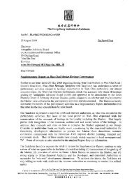
Example <strong>of</strong> UCPs in NUDAPT: Harris County‐Houston<br />
1 km gridded fields from processed digitized lidar data<br />
300<br />
250<br />
Heig ht (m )<br />
200<br />
150<br />
North<br />
West<br />
Northwest<br />
100<br />
50<br />
0<br />
0.000 0.001 0.002 0.003 0.004 0.005 0.006 0.007 0.008 0.009<br />
af(z)<br />
Gridded Frontal Area (packing<br />
density) Index as a function <strong>of</strong><br />
height and approach angle <strong>of</strong><br />
wind (based on Lidar data).<br />
ASI 2: URBAN CLIMATE AND AIR POLLUTION <strong>School</strong> <strong>of</strong> <strong>Architecture</strong>, The Chinese University <strong>of</strong> Hong Kong, Hong Kong, 7-8 Dec 2011<br />
12
ASI2_Lecture 3_7/12/2011<br />
Geo‐Referencing NUDAPT‐44 database for WRF<br />
Large (1 o ) and Small (0.25 o ) Grid Tiles in WPS<br />
ASI 2: URBAN CLIMATE AND AIR POLLUTION <strong>School</strong> <strong>of</strong> <strong>Architecture</strong>, The Chinese University <strong>of</strong> Hong Kong, Hong Kong, 7-8 Dec 2011<br />
rd_wf_binary.f90<br />
Processing steps<br />
NUDAPT into WRF<br />
Intermediate Mesh<br />
Met_em<br />
File<br />
geogrid.exe<br />
real.exe<br />
WRF_input<br />
Module_physics_i<br />
nit<br />
Module_sf_urban<br />
Module_sf_noahdr<br />
y<br />
Call urban_var_init<br />
Use module_sf_urban<br />
Call<br />
BEP_BEM<br />
Call<br />
Module_sf_bep_bem<br />
Module_sf_bep<br />
ASI 2: URBAN CLIMATE AND AIR POLLUTION <strong>School</strong> <strong>of</strong> <strong>Architecture</strong>, The Chinese BEPUniversity <strong>of</strong> Hong Kong, Hong Kong, 7-8 Dec 2011<br />
13
ASI2_Lecture 3_7/12/2011<br />
BEP ‐ 2228 BEP_BEM ‐ 2238<br />
1500 CDT<br />
1900 CDT<br />
2300 CDT<br />
BEP: UHI <strong>of</strong> 1-2<br />
degrees is modeled<br />
during daytime, but<br />
nocturnal UHI was<br />
muted.<br />
BEP_ BEM: Stronger<br />
UHI during day, and<br />
also some UHI during<br />
night, even if after<br />
midnight the UHI<br />
begins to weaken<br />
ASI 2: URBAN CLIMATE AND AIR POLLUTION <strong>School</strong> <strong>of</strong> <strong>Architecture</strong>, The Chinese University <strong>of</strong> Hong Kong, Hong Kong, 7-8 Dec 2011<br />
0300 CDT, 26 August 2006 PBL=8 (Bougeault and Lacarrere)<br />
BEP only: 2228 BEP_BEM: 2238<br />
Introduction <strong>of</strong> NUDAPT enhances the magnitude<br />
and gradients <strong>of</strong> the UHI. The heterogeneities <strong>of</strong><br />
the city are also better represented.<br />
ASI 2: URBAN CLIMATE AND AIR POLLUTION <strong>School</strong> <strong>of</strong> <strong>Architecture</strong>, The Chinese University <strong>of</strong> Hong Kong, Hong Kong, 7-8 Dec 2011<br />
14
ASI2_Lecture 3_7/12/2011<br />
Cooling California Cities:<br />
Cases refer to different ranges <strong>of</strong> increasing albedo<br />
and canopy coverage (surrogate for moisture)<br />
Taha 2008, BLM 127: 218‐239<br />
Delta T (K)<br />
-0.5<br />
-1<br />
-1.5<br />
-2<br />
-2.5<br />
-3<br />
-3.5<br />
-4<br />
San Fernando Valley<br />
0<br />
23<br />
7<br />
15<br />
23<br />
7<br />
15<br />
23<br />
7<br />
15<br />
23<br />
7<br />
15<br />
23<br />
case-01<br />
case-02<br />
case-10<br />
case-20<br />
case-22<br />
LST<br />
Los Angeles<br />
1<br />
0<br />
Delta T (K)<br />
-1<br />
-2<br />
-3<br />
23<br />
-4<br />
7<br />
15<br />
23<br />
7<br />
15<br />
23<br />
7<br />
15<br />
23<br />
7<br />
case-01<br />
15<br />
23<br />
case-02<br />
case-10<br />
case-20<br />
case-22<br />
LST<br />
San Diego<br />
0<br />
Delta T (K)<br />
-0.5<br />
-1<br />
-1.5<br />
-2<br />
-2.5<br />
23<br />
-3<br />
7<br />
15<br />
23<br />
7<br />
15<br />
23<br />
7<br />
15<br />
23<br />
7<br />
15<br />
23<br />
case-01<br />
case-02<br />
case-10<br />
case-20<br />
case-22<br />
LST<br />
ASI 2: URBAN CLIMATE AND AIR POLLUTION <strong>School</strong> <strong>of</strong> <strong>Architecture</strong>, The Chinese University <strong>of</strong> Hong Kong, Hong Kong, 7-8 Dec 2011<br />
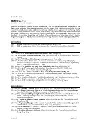
<strong>Air</strong> <strong>Quality</strong> response to UHI modeled modifications:<br />
Comparison against base case for Sacramento CA<br />
Taha 2008: BLM V127: 218‐239<br />
Base case [O3]<br />
Base- Change<br />
(albedo change)<br />
Change in [O3] from base case at time <strong>of</strong> peak.<br />
Increased urban albedo scenario (corresponds to a reduction<br />
<strong>of</strong> 2‐3C in air temperature)<br />
ASI 2: URBAN CLIMATE AND AIR POLLUTION <strong>School</strong> <strong>of</strong> <strong>Architecture</strong>, The Chinese University <strong>of</strong> Hong Kong, Hong Kong, 7-8 Dec 2011<br />
15
ASI2_Lecture 3_7/12/2011<br />
Potential exposure assessment application:<br />
Theory- Pollution retention in urban canyons<br />
Courtesy <strong>of</strong> J. Richmond-Bryant<br />
U<br />
U<br />
WIND<br />
D<br />
l<br />
WIND<br />
D<br />
W<br />
• H = Uτ/D = f(UD/ν, k 0.5 /U, l/D, D/W)<br />
= f(Re, turbulence intensity, shape)<br />
o H = nondimensional residence time <strong>of</strong> pollutant in canyon<br />
o τ = residence time<br />
o k = turbulence kinetic energy <strong>of</strong> the wind<br />
o ν = kinematic viscosity<br />
o Re = Reynolds number<br />
• Based on dimensional analysis and derived from the equation<br />
<strong>of</strong> scalar flux transport (Humphries & Vincent 1976)<br />
ASI 2: URBAN CLIMATE AND AIR POLLUTION <strong>School</strong> <strong>of</strong> <strong>Architecture</strong>, The Chinese University <strong>of</strong> Hong Kong, Hong Kong, 7-8 Dec 2011<br />
Residence time H vs D/W<br />
Courtesy <strong>of</strong> J. Richmond-Bryant<br />
Mid Manhattan05<br />
• Significant fit:<br />
o H = 22(D/W) -0.69<br />
o R 2 = 0.62<br />
o p < 0.001<br />
Two Cities MM and<br />
OkCity<br />
• Poor fit:<br />
o H = 51(D/W) -0.812<br />
o R 2 = 0.035<br />
o p = 0.022<br />
JU2003: OklCity<br />
• Scatter visible<br />
• Novel methodology, under development<br />
• Significant fit:<br />
• Qualitatively similar results for two<br />
o H = 296(D/W) cities<br />
-0.812<br />
o R 2 = 0.48<br />
• Two cities differ quantitatively<br />
o p < 0.0001<br />
• Parameterizations can utilize fine scale<br />
modeling to provide inputs for exposure<br />
assessment<br />
• Improved methodologies with multiple<br />
canopy formulation sets such as from<br />
ASI 2: URBAN CLIMATE AND AIR POLLUTION NUDAPT to be tested.<br />
<strong>School</strong> <strong>of</strong> <strong>Architecture</strong>, The Chinese University <strong>of</strong> Hong Kong, Hong Kong, 7-8 Dec 2011<br />
16
ASI2_Lecture 3_7/12/2011<br />
Crossroads:<br />
Advances and Opportunities<br />
• Urban predictions on now on firmer bases with UCP formulations,<br />
model formulations can become even more sophisticated<br />
• New opportunities (base analyses & “what if” scenarios include:<br />
–Advanced AQ modeling, exposure assessments<br />
–Improved urban dispersion, threat assessments<br />
–UHI assessments, urban climate analyses<br />
–Hydrological and flooding assessments<br />
–Urban design and architecture for ventilation and comfort<br />
analyses<br />
ASI 2: URBAN CLIMATE AND AIR POLLUTION <strong>School</strong> <strong>of</strong> <strong>Architecture</strong>, The Chinese University <strong>of</strong> Hong Kong, Hong Kong, 7-8 Dec 2011<br />
Part 2c: <strong>Fine</strong> <strong>Scale</strong> Modeling Issues<br />
Goal: Realistic outputs from<br />
fine grid WRF mesoscale<br />
modeling.<br />
• Evolution <strong>of</strong> mesoscale<br />
•Capabilities: Available/ growing computer<br />
capabilty/capacity and evolving modeling<br />
system<br />
•Issues: Grid sizes now <strong>of</strong> same order or<br />
smaller as pbl heights, turbulence<br />
(Wyngaard’s “terra Incognita” regime)<br />
•Problems: <strong>Fine</strong> grid modeling needed to<br />
resolve observed features<br />
•Challenges: Determining and removing or<br />
reducing the levels <strong>of</strong> stochastic model noise<br />
•Approaches: WRF with parameterized SG<br />
physics options<br />
WRF with LES<br />
Conduct PULSE Study<br />
ASI 2: URBAN CLIMATE AND AIR POLLUTION <strong>School</strong> <strong>of</strong> <strong>Architecture</strong>, The Chinese University <strong>of</strong> Hong Kong, Hong Kong, 7-8 Dec 2011<br />
17
ASI2_Lecture 3_7/12/2011<br />
WRF modeled vertical velocity at mid‐PBL (~500 m) PBL Eddies<br />
38.7<br />
( courtesy Lemone et al, WRF Workshop, 2011 , updated)<br />
38.1<br />
37.5<br />
36.9<br />
‐98.6 ‐98.0 ‐97.4 ‐96.6 ‐96.0 ‐95.4 ‐98.6 ‐98.0 ‐97.4 ‐96.6 ‐96.0 ‐95.4<br />
38.7<br />
38.1<br />
37.5<br />
36.9<br />
36.3<br />
‐98.6<br />
‐98.0 ‐97.4 ‐96.6 ‐96.0 ‐95.4<br />
‐98.6<br />
‐98.0 ‐97.4 ‐96.6 ‐96.0 ‐95.4<br />
Observations in weakly‐forced convective boundary layers:<br />
Quasi‐stationary 2‐ & 3‐D PBL meteorological fields<br />
http://lance.nasa.gov/imagery/rapid‐response/<br />
Eastern USA, October 2010<br />
Daily summertime occurrence in Houston,TX<br />
area (2006): (MODIS:Terra/Aqua Satellite ~<br />
local noon)<br />
Aug 3 Aug 4<br />
Aug 5<br />
Aug 9 Aug 11 Aug 15<br />
Aug 18 Aug 20 Aug 24<br />
ASI 2: URBAN CLIMATE AND AIR POLLUTION <strong>School</strong> <strong>of</strong> <strong>Architecture</strong>, The Chinese University <strong>of</strong> Hong Kong, Hong Kong, 7-8 Dec 2011<br />
18
ASI2_Lecture 3_7/12/2011<br />
ACM-2<br />
BouLac<br />
QNSE<br />
TKE-NO<br />
TKE-YES<br />
TKE-YES<br />
YSU<br />
TKE-NO<br />
Results Sensitive<br />
to PBL schemes<br />
TERRA: Pixel Size 500m<br />
Aug 4 2006 @ 17:20UTC<br />
Simulations @ 20:00 UTC<br />
MYJ<br />
MYNN2<br />
MYNN3<br />
TKE-YES<br />
TKE-<br />
TKE-<br />
ASI 2: URBAN CLIMATE AND AIR POLLUTION <strong>School</strong> <strong>of</strong> <strong>Architecture</strong>, The Chinese University <strong>of</strong> Hong Kong, Hong Kong, 7-8 Dec 2011<br />
Grid size dependent results<br />
4km(upper) vs 1 km Base (lower)<br />
Heat Flux Latent Heat PBL height Ustar<br />
<strong>Fine</strong> scale structures are unresolved at 4 km, even though features are <strong>of</strong> that order. Resolution becoming<br />
apparent for grids at 1km (or less). From Rampanelli et al., (2004), with 1km grids, shallow circulations can<br />
appear due to convective instability (superadiabatic layer) at the minimum resolved scale (4dx). At the<br />
coarser horizontal grids typical <strong>of</strong> mesoscale models, such circulations would grow too slowly to be noticed.<br />
Hence at 1km the simulations are in a resolution regime where turbulence cannot be explicitly resolved, yet<br />
the superadiabatic ASI 2: URBAN CLIMATE layer can AND induce AIR POLLUTION circulations that <strong>School</strong> grow <strong>of</strong> <strong>Architecture</strong>, to noticeable The Chinese University size over <strong>of</strong> Hong the Kong, integration Hong Kong, 7-8 Dec period. 2011<br />
19
ASI2_Lecture 3_7/12/2011<br />
TERRA: Aug 4 2006 @ 1720 UTC<br />
WRF V3.2 (NOAH BEP_BEM BouLac)<br />
SW Down Base 2238 PBL Base 2238<br />
Martilli’s filter scheme<br />
applied to base case.<br />
SW Down Filtered Base 2238 PBL Filtered Base 2238<br />
Objective: To reduce<br />
amount <strong>of</strong> model noise<br />
ASI 2: URBAN CLIMATE AND AIR POLLUTION <strong>School</strong> <strong>of</strong> <strong>Architecture</strong>, The Chinese University <strong>of</strong> Hong Kong, Hong Kong, 7-8 Dec 2011<br />
Preliminary Study Findings<br />
• Low level convective features are frequent and regular features<br />
in study area for weakly forced systems based on cloud fields<br />
from satellite)<br />
• Convective features are resolvable with fine scale, less so as<br />
grid size increases, characteristics depend on physics options<br />
• Modeled simulations shows convective features to be quasi<br />
stationary<br />
• Spatial characteristic are sensitive to choice <strong>of</strong> physics options.<br />
Presents a significant challenge to modeling air quality at fine<br />
scales<br />
• Ad hoc filtering approaches might be useful towards reducing<br />
model “noise”<br />
• Concern: What is resolved, what is<br />
noise<br />
ASI 2: URBAN CLIMATE AND AIR POLLUTION <strong>School</strong> <strong>of</strong> <strong>Architecture</strong>, The Chinese University <strong>of</strong> Hong Kong, Hong Kong, 7-8 Dec 2011<br />
20
ASI2_Lecture 3_7/12/2011<br />
erturbations nique inks to etup xploration<br />
Taking the model’s<br />
• <strong>Fine</strong> scale modeling enters the “Terra Incognita” regime<br />
• Given that mesoscale modeling systems have many<br />
operating options, how are the resulting simulation<br />
dependent on the user selection <strong>of</strong> model options.<br />
• Need to understand the properties <strong>of</strong> modeling systems<br />
dependence on the properties <strong>of</strong> their individual<br />
components and their linkages.<br />
• Ad hoc modeling group is currently undertaking this study,<br />
preliminary results follows.<br />
• Perform & explore model sensitivity studies including:<br />
Model physics, numerics, time steps, grid size, filtering<br />
ASI 2: URBAN CLIMATE AND AIR POLLUTION <strong>School</strong> <strong>of</strong> <strong>Architecture</strong>, The Chinese University <strong>of</strong> Hong Kong, Hong Kong, 7-8 Dec 2011<br />
Numerical Considerations: Horizontal Diffusion<br />
Standard configuration <strong>of</strong> WRF has in the horizontal the Smagorinsky scheme<br />
K<br />
h<br />
s<br />
C x<br />
2<br />
s<br />
C 0.4<br />
2<br />
u<br />
v<br />
<br />
0.25<br />
2 2 <br />
<br />
<br />
x<br />
y<br />
<br />
ASI 2: URBAN CLIMATE AND AIR POLLUTION <strong>School</strong> <strong>of</strong> <strong>Architecture</strong>, The Chinese University <strong>of</strong> Hong Kong, Hong Kong, 7-8 Dec 2011<br />
2<br />
2<br />
u<br />
v<br />
<br />
<br />
<br />
y<br />
x<br />
<br />
<br />
In Martilli’s simulations, with DX=1km, this gives K h values <strong>of</strong> the order <strong>of</strong> 100-200 m2/s<br />
Standard MM5 has in the horizontal (see Xu et al. MWR 2001)<br />
K<br />
K<br />
h<br />
H 0<br />
K<br />
H 0<br />
3. 10<br />
2<br />
2<br />
<br />
2 2 u<br />
v<br />
u<br />
v<br />
<br />
Cs<br />
x<br />
0.25<br />
2 2 <br />
<br />
<br />
x y<br />
<br />
<br />
y x<br />
<br />
<br />
3<br />
x<br />
t<br />
2<br />
2<br />
600.<br />
m 2 //s<br />
s<br />
For Dx=1000.m and Dt=5s (Martilli’s case)<br />
“the background term K H0 is dominant at all levels and locations<br />
throughout the simulation time” Xu et al. MWR 2001<br />
21
ASI2_Lecture 3_7/12/2011<br />
WRF simulations over Madrid (1 km resolutión) 1200 UTC<br />
K H Smagorinsky Smagorinsky CONST: With K HO =600 m 2 /s (MM5 style)<br />
Temperature<br />
(2m)<br />
CONST<br />
Vertical velocities<br />
(250m)<br />
Vertical<br />
velocity<br />
ASI 2: URBAN CLIMATE AND AIR POLLUTION <strong>School</strong> <strong>of</strong> <strong>Architecture</strong>, The Chinese University <strong>of</strong> Hong Kong, Hong Kong, 7-8 Dec 2011<br />
Alternative methodology:<br />
In addition to filtering structures smaller than the grid cell, we also<br />
filter turbulent eddies smaller than the size <strong>of</strong> the most energetic<br />
eddies. Because we are running in RANS mode, all turbulence should<br />
be filtered out by the turbulence closure scheme. Martilli’s choice is<br />
to improve the treatment <strong>of</strong> the horizontal turbulent transport terms.<br />
u<br />
uu<br />
uv<br />
uw<br />
P<br />
uu<br />
uv<br />
uw<br />
<br />
t<br />
x<br />
y<br />
z<br />
x<br />
x<br />
y<br />
z<br />
Mean advection and pressure: resolved<br />
Can we still neglect these terms for high<br />
resolution (1km or less) runs<br />
Horizontal turbulent<br />
transport: neglected<br />
Vertical turbulent transport:<br />
parameterized<br />
Some ad hoc<br />
horizontal diffusion<br />
is <strong>of</strong>ten added<br />
Try to parameterize them: if they are not relevant they will show no impact on the<br />
ASI 2: URBAN CLIMATE AND AIR POLLUTION <strong>School</strong> results. <strong>of</strong> <strong>Architecture</strong>, The Chinese University <strong>of</strong> Hong Kong, Hong Kong, 7-8 Dec 2011<br />
22
ASI2_Lecture 3_7/12/2011<br />
Suggested parameterization<br />
u u <br />
u u K<br />
<br />
i j 2<br />
Best option would be to treat <br />
<br />
i j<br />
ijtke<br />
x<br />
j<br />
x <br />
<br />
<br />
i <br />
3<br />
As first step, Martilli assumed<br />
ui<br />
u<br />
iuj<br />
K<br />
Relatively easy to implement in WRF….<br />
x<br />
j<br />
For “ K” Martilli invoked the Bougeault and Lacarrere scheme, so<br />
the vertical diffusion coefficient becomes<br />
K<br />
z<br />
<br />
cl<br />
boulac<br />
tke<br />
By analogy, in the horizontal<br />
K c maxl<br />
, x tke<br />
x<br />
boulac<br />
<br />
z<br />
zdz<br />
tkez<br />
<br />
down<br />
<br />
z<br />
zdz<br />
tkez<br />
<br />
z o<br />
1/<br />
2<br />
l<br />
upldown<br />
<br />
minl<br />
,l <br />
ASI 2: URBAN CLIMATE AND AIR POLLUTION <strong>School</strong> <strong>of</strong> <strong>Architecture</strong>, The Chinese University <strong>of</strong> Hong Kong, Hong Kong, 7-8 Dec 2011<br />
z<br />
<br />
zlup<br />
z<br />
zl<br />
l<br />
l<br />
<br />
boulac<br />
g<br />
o<br />
g<br />
up<br />
down<br />
l up and l down are the distances that a parcel<br />
originating from level z, and having the<br />
TKE <strong>of</strong> level z, can travel upward and<br />
downward before coming to rest due to<br />
buoyancy effects.<br />
Application <strong>of</strong> Filter Option<br />
Base<br />
New<br />
23
ASI2_Lecture 3_7/12/2011<br />
Model study <strong>of</strong> Vortices in high-resolution WRF<br />
Courtesy <strong>of</strong> E. Gutierrez, J. Gonzalez, CCNY, & R. Bornstein, SJSU<br />
Simulations <strong>of</strong> a 2010 NYC Heat Wave: Real or Noise<br />
z=12 m, 18 EST; coarse domain, ∆x=9 km, ∆t = 1 s:<br />
Temperature (12m)<br />
W velocity (12m)<br />
Reasonable results, but not much detail<br />
ASI 2: URBAN CLIMATE AND AIR POLLUTION <strong>School</strong> <strong>of</strong> <strong>Architecture</strong>, The Chinese University <strong>of</strong> Hong Kong, Hong Kong, 7-8 Dec 2011<br />
Sensitivity to ∆x<br />
Temperature (12m)<br />
∆t fixed at 1 s<br />
Vertical velocity (12m)<br />
∆X=1 km<br />
∆X=333 m<br />
∆X=1 km<br />
∆X=333 m<br />
W (12m) X-section thru<br />
Manhattan<br />
∆X=1 km<br />
∆X=333 m<br />
ASI 2: URBAN CLIMATE AND AIR POLLUTION <strong>School</strong> <strong>of</strong> <strong>Architecture</strong>, The Chinese University <strong>of</strong> Hong Kong, Hong Kong, 7-8 Dec 2011<br />
24
ASI2_Lecture 3_7/12/2011<br />
Sensitivity to ∆t; ∆x = 1 km<br />
Vertical Velocity x-section through Manhattan<br />
∆t=6 s<br />
∆t=1 s<br />
∆t=0.66 s<br />
∆t=0.11 s<br />
ASI 2: URBAN CLIMATE AND AIR POLLUTION <strong>School</strong> <strong>of</strong> <strong>Architecture</strong>, The Chinese University <strong>of</strong> Hong Kong, Hong Kong, 7-8 Dec 2011<br />
Terra Incognita<br />
LES and mesoscale limits<br />
From Wyngaard<br />
•If the (integral) scale <strong>of</strong> the turbulence is l, then in the LES limit, i.e., ∆ ≪ l, the numerical grid resolves all <strong>of</strong> the<br />
energy-containing turbulence.<br />
•The subgrid model is responsible only for energy transfer from the resolved scales. The standard Smagorinsky<br />
(or Lilly) subgrid model produces this transfer at the correct mean rate.<br />
•In the mesoscale limit, ∆ ≫ l, no turbulence is resolved. Turbulence effects are represented through a subgrid<br />
model, typically <strong>of</strong> the ensemble-mean type. In principle the subgrid model can be adjusted to perform well in this<br />
limit.<br />
•Between these two limits lies the Terra Incognita where the subgrid model carries significant fluxes and<br />
transfers energy. In principle neither ensemble mean nor the traditional LES closures are appropriate there.<br />
ASI 2: URBAN CLIMATE AND AIR POLLUTION <strong>School</strong> <strong>of</strong> <strong>Architecture</strong>, The Chinese University <strong>of</strong> Hong Kong, Hong Kong, 7-8 Dec 2011<br />
25
ASI2_Lecture 3_7/12/2011<br />
Summary: <strong>Fine</strong> grid modeling issues<br />
• A Conundrum: Real features <strong>of</strong> 1-10 km scales require grid resolution<br />
about an order <strong>of</strong> magnitude finer in size; however, much stochastic<br />
noise is present in current mesoscale simulations at fine scales (Terra<br />
Incognita regime).<br />
• Quasi Stationary, persistent 2-D and 3-D circulation in weakly forced flows<br />
• Simulations are physics option dependent<br />
• K H using SMAG (allows rolls), K H SMAG + Constant (supresses rolls)<br />
• Horizontal vortices and/or structures:<br />
– Become more pronounced with decreasing ∆x = 1km, 333m & 111m<br />
– Dissipate for decreasing ∆t= 6s,1s, 0.66s, 0.33s (features are non convergent)<br />
– Reaches max strength in afternoon, dissipate at night, are computationally stable<br />
• Numerical filters may helpful in reducing stochastic model noise, but<br />
there is no fundamental guidance that currently apply.<br />
• Other aspects/sensitivities, approaches still need to be explore:<br />
Even vs odd order filters.<br />
WRF LES<br />
ASI 2: URBAN CLIMATE AND AIR POLLUTION <strong>School</strong> <strong>of</strong> <strong>Architecture</strong>, The Chinese University <strong>of</strong> Hong Kong, Hong Kong, 7-8 Dec 2011<br />
Part 3: <strong>Fine</strong> grid air quality modeling (examples CMAQ)<br />
1 km UCP 4km Native<br />
Ozone NOx<br />
• 1 km results are<br />
significantly more<br />
textured than 4<br />
km<br />
• The titrating effect<br />
<strong>of</strong> NOx on ozone<br />
(especially along<br />
highways and<br />
major point<br />
sources) are<br />
captured at 1km<br />
but not at 4 km<br />
• Photochemistry at<br />
4 km results in<br />
part from overdilution<br />
<strong>of</strong> withingrid<br />
sources<br />
ASI 2: URBAN CLIMATE AND AIR POLLUTION <strong>School</strong> <strong>of</strong> <strong>Architecture</strong>, The Chinese University <strong>of</strong> Hong Kong, Hong Kong, 7-8 Dec 2011<br />
26
ASI2_Lecture 3_7/12/2011<br />
Dependence on UCP<br />
Ozone (1 km grid CMAQ simulations) @ 2100 GMT<br />
UCP no_UCP ∆ (UCP-no_UCP)<br />
• Significant differences in the spatial patterns shown between<br />
UCP and noUCP runs (titration effect occurs in both sets)<br />
• Flow, thermodynamics & turbulent fields differ between the<br />
UCP and noUCP simulations & contribute to differences<br />
ASI 2: URBAN CLIMATE AND AIR POLLUTION <strong>School</strong> <strong>of</strong> <strong>Architecture</strong>, The Chinese University <strong>of</strong> Hong Kong, Hong Kong, 7-8 Dec 2011<br />
Simulations are unique to grid size:<br />
Example: Ozone: <strong>Fine</strong> vs Coarse (2100 GMT)<br />
Aggregate: 4km mean<br />
from 1km (w/ucp)<br />
Native 4 km simulation<br />
∆ (Aggregate-Native)<br />
• Differences between Mean 4km aggregated from 1 km vs Native 4km<br />
• Accumulative and net <strong>of</strong> atmospheric processes acting on 1 km scale<br />
differs from that at 4km scale<br />
ASI 2: URBAN CLIMATE AND AIR POLLUTION <strong>School</strong> <strong>of</strong> <strong>Architecture</strong>, The Chinese University <strong>of</strong> Hong Kong, Hong Kong, 7-8 Dec 2011<br />
27
ASI2_Lecture 3_7/12/2011<br />
Characterizing, Modeling Sub-Grid Features<br />
Ching and Majeed, 2011<br />
Increasing level <strong>of</strong> detail <strong>of</strong> the pollutant concentration distribution possible with<br />
decreasing model grid size.<br />
In principle, even finer concentration detail occur below 1 km grid simulations.<br />
Histogram <strong>of</strong> concentrations is derived from nested grid concentration simulations.<br />
ASI 2: URBAN CLIMATE AND AIR POLLUTION <strong>School</strong> <strong>of</strong> <strong>Architecture</strong>, The Chinese University <strong>of</strong> Hong Kong, Hong Kong, 7-8 Dec 2011<br />
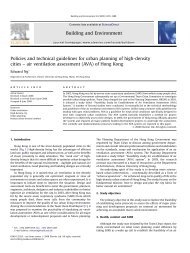
Two-parameter Weibull probability density function<br />
Hereinafter “Distribution Function”<br />
k > 0 is the shape parameter<br />
λ > 0 is the scale parameter<br />
ASI 2: URBAN CLIMATE AND AIR POLLUTION <strong>School</strong> <strong>of</strong> <strong>Architecture</strong>, The Chinese University <strong>of</strong> Hong Kong, Hong Kong, 7-8 Dec 2011<br />
28
ASI2_Lecture 3_7/12/2011<br />
HCHO Histograms and fitted Weibull distributions<br />
12km grids, Wilmington Delaware July 2001. Based on 1km CMAQ<br />
ASI 2: URBAN CLIMATE AND AIR POLLUTION <strong>School</strong> <strong>of</strong> <strong>Architecture</strong>, The Chinese University <strong>of</strong> Hong Kong, Hong Kong, 7-8 Dec 2011<br />
1.2<br />
1<br />
Cell11:2<br />
Cell12:2<br />
Wilmington - Weibull <strong>Scale</strong> Factors<br />
Cell11:3<br />
Cell12:3<br />
0.8<br />
0.6<br />
0.4<br />
0.2<br />
0<br />
1 101 201<br />
Time<br />
301<br />
(Hours)<br />
401 501 601<br />
25<br />
20<br />
Wilmington - Weibull Shape Factors<br />
Cell11:2<br />
Cell12:2<br />
Cell11:3<br />
Cell12:3<br />
Shape Factor<br />
15<br />
10<br />
5<br />
0<br />
1 101 201 301 401 501 601<br />
Time (Hours)<br />
ASI 2: URBAN CLIMATE AND AIR POLLUTION <strong>School</strong> <strong>of</strong> <strong>Architecture</strong>, The Chinese University <strong>of</strong> Hong Kong, Hong Kong, 7-8 Dec 2011<br />
29
ASI2_Lecture 3_7/12/2011<br />
Cell row: Cell column R 2<br />
Regression model <strong>of</strong> Shape & <strong>Scale</strong><br />
Wilmington grid cell 11:2<br />
Shape Linear-form Log-form<br />
11:2 (SW) 0.26 0.28<br />
11:3 (SE) 0.27 0.35<br />
12:2 (NW) 0.18 0.17<br />
12:3 (NE) 0.08 0.09<br />
Cell row: Cell column R 2<br />
<strong>Scale</strong> Linear-form Log-form<br />
11:2 (SW) 0.65 0.73<br />
11:3 (SE) 0.62 0.81<br />
12:2 (NW) 0.65 0.77<br />
12:3 (NE) 0.68 0.80<br />
C 12km = Concentration (12-km cell value)<br />
E 12km = Emissions (12-km cell value)<br />
σ E1km = Std. Dev. <strong>of</strong> Emission (based on 1-km cell<br />
value)<br />
Skew E1km = Skewness <strong>of</strong> Emission (based on 1-km cell<br />
value)<br />
Kurt E1km = Kurtosis <strong>of</strong> Emission (based on 1-km cell value)<br />
U* 12km = Ustar (12-km cell value)<br />
W* 12km = Wstar (12-km cell value)<br />
PBL 12km = PBL height (12-km cell value)<br />
WS10 12km = 10m Wind Speed (12-km cell value)<br />
WD10 12km = 10m Wind Direction (12-km cell value)<br />
T10 12km = 10m Temperature (12-km cell value)<br />
Q10 12km = 10m Mixing Ratio (12-km cell value)<br />
Linear form:<br />
Shape = 0.28+0.33 C 12km -0.19 E 12km +0.26 σ E1km -0.74Skew E1km +0.75Kurt E1km -0.33 U* 12km +0.10PBL 12km<br />
+0.36WS10 12km -0.09WD10 12km -0.14T10 12km +0.08Q10 12km<br />
<strong>Scale</strong> = 0.13+0.69 C 12km +0.11 E 12km -0.04Kurt E1km -0.27U* 12km +0.21W* 12km -0.10 PBL 12km + 0.04 T10 12km<br />
Logarithmic form:<br />
Shape = -0.22+0.37 C 12km –7.4x10 -05 E 12km -0.33 σ E1km -0.30k E12km +1.50Skew E1km +0.77Kurt E1km<br />
+0.14WS10 12km -0.01WD10 12km -0.17Q10 12km<br />
<strong>Scale</strong> = 1.25+0.74 C 12km +4.8x10 -05 E 12km +0.08 σ E1km -1.34k E12km 2.60Skew E1km +0.74Kurt E1km -0.19WS10 12km<br />
ASI 2: URBAN -0.01WD10 CLIMATE 12km AND -0.07Q10 AIR POLLUTION 12km,<br />
<strong>School</strong> <strong>of</strong> <strong>Architecture</strong>, The Chinese University <strong>of</strong> Hong Kong, Hong Kong, 7-8 Dec 2011<br />
Fitted Shape and <strong>Scale</strong> vs regression model<br />
1<br />
0.8<br />
0.6<br />
Series1<br />
Series2<br />
Series3<br />
0.4<br />
0.2<br />
0<br />
‐0.2<br />
1 101 201 301 401 501 601<br />
‐0.4<br />
1<br />
0.8<br />
0.6<br />
0.4<br />
0.2<br />
0<br />
‐0.2<br />
Series1<br />
Series2<br />
Series3<br />
1 101 201 301 401 501 601<br />
Shape based on Regression<br />
1<br />
0.8<br />
0.6<br />
0.4<br />
0.2<br />
0<br />
0 0.2 0.4 0.6 0.8 1<br />
‐0.4<br />
Best it Shape<br />
ASI 2: URBAN CLIMATE AND AIR POLLUTION <strong>School</strong> <strong>of</strong> <strong>Architecture</strong>, The Chinese University <strong>of</strong> Hong Kong, Hong Kong, 7-8 Dec 2011<br />
30
ASI2_Lecture 3_7/12/2011<br />
SGV parameterization model<br />
• Framework and template based upon a given ensemble set <strong>of</strong> a<br />
priori simulations.<br />
• Framework and template designed to provide on-line<br />
complimentary gridded output to coarse (operational) CMAQ<br />
simulations<br />
• Given growing availability <strong>of</strong> annual regional-scale CMAQ<br />
simulations, a similar approach could be satisfactorily applied<br />
and extended to very coarse grid scales, e.g., global and<br />
climate model simulations.<br />
• Potential for population exposure assessment application<br />
• Model evaluation and “Weight <strong>of</strong> Evidence” regulatory<br />
applications<br />
ASI 2: URBAN CLIMATE AND AIR POLLUTION <strong>School</strong> <strong>of</strong> <strong>Architecture</strong>, The Chinese University <strong>of</strong> Hong Kong, Hong Kong, 7-8 Dec 2011<br />
• Modeling meso‐scale to urban‐scale features requires care when selecting sets <strong>of</strong><br />
modeling parameterizations; one size (set) may not fit all!<br />
• There are currently a variety <strong>of</strong> modeling approaches for the urban canopy ranging<br />
from slab (Reynolds averaging) to single and multiple canopy layers. Each<br />
approach has advantages and limitations, strengths and weaknesses, and its<br />
suitability may be more dependent on the required application (“Fit for Purpose”<br />
quoting Martilli).<br />
• Model results are sensitive to the choice <strong>of</strong> grid size and parameterization<br />
schemes; model evaluation approaches will need to be robust and requiring<br />
specialized datasets.<br />
• Requirements for urban modeling can differ significantly from that <strong>of</strong> meso‐scale<br />
for urban canopies that are deep and complex.<br />
• The modeling results depicting characteristic fine scale spatial structure is not as<br />
yet verified. Some important and critical issues remain to be resolved regarding<br />
simulation in the Terra Incognita regime).<br />
• Advanced urban modeling makes possible numerical experiments for predicting<br />
changes in the urban climate, UHI, and air quality <strong>of</strong> urban environments.<br />
• Databases <strong>of</strong> buildings are becoming increasingly available facilitating realization <strong>of</strong><br />
operational feasibility for modeling meteorology and air quality for individual<br />
cities.<br />
• The modeling framework supporting urban scale modeling is emerging, but the<br />
science bases and insights are growing rapidly.<br />
ASI 2: URBAN CLIMATE AND AIR POLLUTION <strong>School</strong> <strong>of</strong> <strong>Architecture</strong>, The Chinese University <strong>of</strong> Hong Kong, Hong Kong, 7-8 Dec 2011<br />
31
ASI2_Lecture 3_7/12/2011<br />
Thank You<br />
Contact information:<br />
Jason Ching<br />
University <strong>of</strong> North Carolina<br />
Institute for the Environment CB6116<br />
(137 E. Franklin St, Chapel Hill, NC, USA 27599)<br />
Email: jksching@gmail.com<br />
ASI 2: URBAN CLIMATE AND AIR POLLUTION <strong>School</strong> <strong>of</strong> <strong>Architecture</strong>, The Chinese University <strong>of</strong> Hong Kong, Hong Kong, 7-8 Dec 2011<br />
32