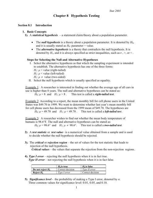
Chapter 8 Hypothesis Testing

Chapter 8 Hypothesis Testing
Stat 2601
Section 8.1
Introduction
1. Basic Concepts
1). A statistical hypothesis – a statement/claim/theory about a population parameter.
The null hypothesis is a theory about a population parameter. It is denoted by H 0 ,
and it is usually stated as H 0 : parameter = value.
The alternative hypothesis is a theory that contradicts the null hypothesis. It is
denoted by H 1 , and it is always specified as strict inequalities, such as , >, or < .
Steps for Selecting the Null and Alternative Hypotheses
I. Select the alternative hypothesis as that which the sampling experiment is intended
to establish. The alternative hypothesis has one of the three forms:
H 1 : μ > value (right-tailed)
H 1 : μ < value (left-tailed)
H 1 : μ value (two-sided)
II. Select the null hypothesis which is usually specified as equality.
Example 1: A researcher is interested in finding out whether the average age of all cars in
use is higher than 8 years. The null and alternative hypotheses can be stated as:
H 0 : μ = 8 and H 1 : μ > 8 . This test is called a right-tailed test.
Example 2: According to a report, the mean monthly bill for cell phone users in the United
States was $49.70 in 1999. We want to determine whether last year’s mean monthly bill
for cell phone users has decreased from the 1999 mean of $49.70. The hypotheses are
H 0 : μ = 49.70 and H 1 : μ < 49.70 . This test is called a left-tailed test.
Example 3: A researcher wishes to find out whether the mean body temperature of
humans is 98.6°F. The null and alternative hypotheses can be stated as:
H 0 : μ = 98.6° and H 1 : μ 98.6°. This test is called a two-tailed test.
2). A test statistic or test value– is a numerical value obtained from a sample and is used
to decide whether the null hypothesis should be rejected.
3). The critical or rejection region – the set of values for the test statistic that leads to
rejection of the null hypothesis.
Critical values – the values that separate the rejection from the non-rejection regions.
4). Type I error – rejecting the null hypothesis when it is in fact true.
Type II error – not rejecting the null hypothesis when it is in fact false.
H 0 is true
H 0 is false
Do not reject H 0 Correct decision Type II error
Reject H 0 Type I error Correct decision
5). Significance level - the probability of making a Type I error, denoted by α.
Three common values for significance level: 0.01, 0.05, and 0.10.
1

Section 8.2
z Test for a Mean (Traditional Method and P-value Method)
Stat 2601
1. Definition
The z test is a statistical test which can be used when the population standard deviation is
known and the population is normally distributed or when n ≥ 30. The test statistic for a z
test with null hypothesis H 0 : μ = μ 0 is:
X
z
0 .
/ n
2. Traditional Method (Critical-Value Method) for Hypothesis Testing
1) Steps:
State the hypotheses.
Compute the value of the test statistic.
Find the rejection region at a specified significance level α.
Make the decision to reject or not reject H 0 .
Interpret the results of the hypothesis test.
2) Finding the Rejection Region for a Specific α value when a z-test is
performed.
a) Right-tailed
Rejection region: z > z α , where z α is a z value that will give an area of α in the
right tail of the standard normal distribution. z α is also called the critical value, a
value that separates the rejection region and non-rejection region.
If α = .05, the rejection region is z > 1.645.
Right tail area α
0
C.V.
b) Left-tailed
For a left-tailed test, the rejection region: z < -z α .
When α=.05, the C.V. is -1.645, the rejection region is z < -1.645
.
0
2

Stat 2601
c) Two-sided
For a two-sided test, the rejection region: z > z α/2 or z < -z α/2 .
When α=.05., the rejection region is z > 1.96 or z < -1.96.
Total tail area =
0
Table 8.1 Summary of rejection region at a specific significance level α
Rejection Region
Upper-tailed Lower-tailed Two-sided
α = .01 z > 2.33 z < -2.33 z > 2.575 or z < -2.575
α = .05 z > 1.645 z < -1.645 z > 1.96 or z < -1.96
α = .1 z > 1.28 z < -1.28 z > 1.645 or z < -1.645
Example 1: A researcher is interested in finding out whether the average age of all
cars in use is higher than 8 years. A random sample of 40 cars were selected and the
average age of cars was found to be 8.5 yrs, and the standard deviation was 3.5 yrs. At
α=.05, can it be concluded that the average age of all cars in use is higher than 8 years
Example 2: According to a report, the mean monthly bill for cell phone users in the
United States was $49.70 in 1999. We want to determine whether last year’s mean
monthly bill for cell phone users has decreased from the 1999 mean of $49.70. A
random sample of 50 sample users was selected and average of the last year’s monthly
cell phone bills for these 50 users was $41.40. At the 1% significance level, do we have
enough evidence to conclude that last year’s mean monthly bill for cell phone users has
decreased from the 1999 mean of $49.70 Assume that σ = 25.
3

Stat 2601
Example 3: A researcher wishes to find out whether the mean body temperature of
humans is 98.6° F. The researcher obtained the body temperature of 93 healthy humans
and found that the mean body temperature is 98.1°F. At the 1% significance level, do
the data provide sufficient evidence to conclude that the mean body temperature of
healthy humans differs from 98.6°F. Assume that σ = .63°F.
3. P-value Method
1) Definition
P-value- the P-value of a hypothesis test is the probability of observing a value of
the test statistic as extreme or more extreme than that observed when the null
hypothesis is true.
Right-tailed test: The P-value is the probability of observing a value of the test
statistic as large as or larger than the value actually observed, which is the area
under the standard normal curve that lies to the right of the observed test statistic.
Left-tailed test: The P-value is the probability of observing a value of the test
statistic as small as or smaller than the value actually observed.
Two-sided test: The P-value is the probability of observing a value of the test
statistic at least as large in magnitude as the value actually observed.
2) Steps
State the hypotheses.
Compute the value of the test statistic, say z 0 .
Find the P-value.
For an upper-tailed test, P-value = P(z > z 0 ).
For a lower -tailed test, P-value = P(z < z 0 ).
For a two-sided test, P-value = 2*P(z > z 0 ) if z 0 > 0,
or = 2*P(z < z 0 ) if z 0 < 0.
If P –value ≤ α, reject H 0 ; otherwise, do not reject H 0 .
Interpret the results of the hypothesis test.
Example 1: Use the P-value method to perform the same hypothesis test.
4

Stat 2601
Example 2 Use the P-value method to perform the same hypothesis test.
Example 3: Use the P-value method to perform the same hypothesis test.
Section 8.3
t Test for a Mean
1. Definition
The t test is a statistical test which can be used when the population is normally
distributed, σ is unknown and n < 30. The test statistic for a t test with null hypothesis
H 0 : μ = μ 0 is:
X
t
0 .
s / n
The degrees of freedom are d.f. = n -1.
2. Finding the rejection region
1) H 1 : µ > µ 0 , rejection region: t > t α .
2) H 1 : µ < µ 0 , rejection region: t t α/2 or t < -t α/2 .
Where t α .is the t-value that will give an area of α to its right. t α .and t α/2 are based
on (n-1) df.
Example: The average undergraduate cost for tuition, fees, and room for two-year
institutions last year was $13,252. The following year, a random sample of 20 two-year
institutions had a mean of $15,560 and a standard deviation of $3500. Is there sufficient
evidence at α = .05 to conclude that the mean cost has increased
5

Section 8.4
z Test for a Proportion
Stat 2601
1. The test statistic for a test of hypothesis with H 0 : p = p 0 is:
z
pˆ
p
0
p0
,
q / n
Where pˆ is the sample proportion, n is the sample size, p 0 is the hypothesized value of p.
2. Rejection region (Traditional method)
See Table 8.1.
3. p-value (p-value method)
See Section 8.2.
0
Example 8.4.1: A recent survey found that 64.7% of the population owns their homes. In a
random sample of 150 heads of household, 92 responded that they owned their homes. At the
0.01 level of significance, does that indicate a difference from the national proportion Use
the traditional method.
Example 8.4.2: Nationally 60.2% of federal prisoners are serving time for drug offenses. A
warden feels that in his prison the percentage is even higher. He surveys 400 inmates’
records and finds that 260 of the inmates are drug offenders. At α = 0.05, is he correct Use
the P-value method.
6