One Sample T-test

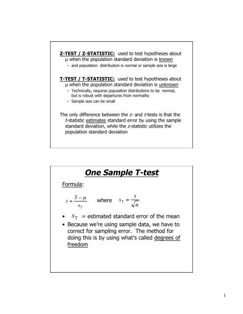
Z-TEST / Z-STATISTIC: used to test hypotheses about
µ when the population standard deviation is known
– and population distribution is normal or sample size is large
T-TEST / T-STATISTIC: used to test hypotheses about
µ when the population standard deviation is unknown
– Technically, requires population distributions to be normal,
but is robust with departures from normality
– Sample size can be small
The only difference between the z- and t-tests is that the
t-statistic estimates standard error by using the sample
standard deviation, while the z-statistic utilizes the
population standard deviation
Formula:
One Sample T-test
t
=
x − µ
s x
where
s x
=
s
n
s x
• = estimated standard error of the mean
• Because we’re using sample data, we have to
correct for sampling error. The method for
doing this is by using what’s called degrees of
freedom
1

Degrees of Freedom
• degrees of freedom ( ) are defined as the number of
scores in a sample that are free to vary
• we know that in order to calculate variance we must
know the mean ( )
• this limits the number of scores that are free to vary
df = n −1
X
s =
df
∑( x i
− x )
n −1
•
€
where is the number of
scores in the sample
n
Degrees of Freedom Cont.
Picture Example
•There are five balloons:
one blue, one red, one
yellow, one pink, & one
green.
•If 5 students (n=5) are
each to select one
balloon only 4 will have
a choice of color (df=4).
The last person will get
whatever color is left.
2

• The particular t-distribution to use depends
on the number of degrees of freedom(df)
there are in the calculation
• Degrees of freedom (df)
– df for the t-test are related to sample size
– For single-sample t-tests, df= n-1
– df count how many observations are free to vary
in calculating the statistic of interest
• For the single-sample t-test, the limit is
determined by how many observations can
vary in calculating s in
t obt
= x − µ
s
n
€
z obt
= x − µ
σ
n
€
The z-test assumes that:
• the numerator varies from
one sample to another
• the denominator is constant
Thus, the sampling
distribution of z derives
from the sampling
distribution of the mean
Z-test vs. T-test
€
t obt
= x − µ
s
n
The z-test assumes that:
• the numerator varies from one
sample to another
• the denominator varies from
one sample to another
• Therefore the sampling
distribution is broader than
it otherwise would be
• The sampling distribution
changes with n
• It approaches normal as n
increases
3

Characteristics of the t-distribution:
• The t-distribution is a family of distributions --
a slightly different distribution for each
sample size (degrees of freedom)
• It is flatter and more spread out than the
normal z-distribution
• As sample size increases, the t-distribution
approaches a normal distribution
Introduction to the t-statistic
3.5
3
t-dist., df=5
2.5
Normal Distribution,
df=∞
t-dist., df=20
2
1.5
1
t-dist., df=1
0.5
0
-3 -2 -1 0 1 2 3
When df are large the curve approximates the normal
distribution. This is because as n is increased the
estimated standard error will not fluctuate as much
between samples.
4

• Note that the t-statistic is analogous to the z-
statistic, except that both the sample mean and
the sample s.d. must be calculated
• Because there is a different distribution for
each df, we need a different table for each df
– Rather than actually having separate tables for each
t-distribution, Table D in the text provides the critical
values from the tables for df= 1 to df= 120
– As df increases, the t-distribution becomes
increasingly normal
– For df=∞, the t-distribution is
Procedures in doing a t-test
1. Determine H 0 and H 1
2. Set the criterion
Look up t crit , which depends on alpha and df
3. Collect sample data, calculate x and s
4. Calculate the test statistic
t obt
= x − µ
s
n
5. Reject H 0 if t obt is more extreme than
t crit€
5

Example:
A population of heights has a µ=68. What is the
probability of selecting a sample of size n=25 that
has a mean of 70 or greater and a s=4
• We hypothesized about a population of
heights with a mean of 68 inches. However,
we do not know the population standard
deviation. This tells us we must use a t-test
instead of a z-test
Step 1: State the hypotheses
H 0 : µ=68
H 1 : µ≥68
6

Step 2: Set the criterion
• one-tail test or two-tail test
• α=
• df = n-1 =
• See table for critical t-value
Step 3: Collect sample data, calculate x
and s
From the example we know the sample mean is 70,
with a standard deviation (s) of 4.
Step 4: Calculate the test statistic
• Calculate the estimated standard error of the
mean
s x
= s n = 4 25 = 0.8
€
• Calculate the t-statistic for the sample
x − µ
t =
t =
s x
70 − 68
0.8
= 2.5
€
7

Step 5: Reject H 0 if t obt is more extreme
than t crit
• The critical value for a one-tailed t-test with
df=24 and α=.05 is 1.711
• Will we reject or fail to reject the null
hypothesis
4
3
2
1
0
t crit =1.711
0.05
Example:
A researcher is interested in determining whether or
not review sessions affect exam performance.
The independent variable, a review session, is
administered to a sample of students (n=9) in an
attempt to determine if this has an effect on the
dependent variable, exam performance.
Based on information gathered in previous semesters,
I know that the population mean for a given exam is
24.
The sample mean is 25, with a standard deviation (s)
of 4.
8

• We hypothesized about a population mean
for students who get a review based on the
information from the population who didn’t
get a review (µ=24). However, we do not
know the population standard deviation. This
tells us we must use a t-test instead of a z-
test
Step 1: State the hypotheses
H 0 : µ=24
H 1 : µ≥24
Step 2: Set the criterion
• one-tail test or two-tail test
• α=
• df = n-1 =
• See table for critical t-value
Step 3: Collect sample data, calculate x
and s
From the example we know the sample mean is 25,
with a standard deviation (s) of 4.
9

Step 4: Calculate the test statistic
• Calculate the estimated standard error of the
mean
s 4 4
s x
= = = = 1.33
n 9 3
• Calculate the t-statistic for the sample
x − µ
t =
s
26 − 24
t = =
1.33
x
2
1.33
= 1.503
Step 5: Reject H 0 if t obt is more extreme
than t crit
• The critical value for a one-tailed t-test with
df=8 and α=.05 is 1.86
• Will we reject or fail to reject the null
hypothesis
4
3
2
1
0
0.025
t crit =-2.101
− α 2
t + α crit =2.101
2
0.025
€
€
10

Assumptions of the t-Test:
• Independent Observations: Each person’s
score in the sample is not affected by other
scores; if, for example, 2 subjects cheated
from one another on the exam, the
independence assumption would be violated
• Normality: The population sampled must be
normally distributed
• Need to know only the population mean
• Need sample mean and standard deviation
Confidence Intervals
• Often, one’s interest is not in testing a hypothesis,
but in estimating a population mean or proportion
– This cannot be done precisely, but only to some extent
– Thus, one estimates an interval, not a point value
– The interval contains the true value with a probability
– The wider the interval, the greater the probability that it
contains the true value
• Thus there is a precision/confidence trade-off
• The intervals are called confidence intervals(CI)
• Typical CIs contain the true value with probability
.95 (95% CI) and with probability .99 (99% CI)
• CI is calculated with either t or z, as appropriate
11