Diamond Detectors for Ionizing Radiation - HEPHY
Diamond Detectors for Ionizing Radiation - HEPHY
Diamond Detectors for Ionizing Radiation - HEPHY

Create successful ePaper yourself
Turn your PDF publications into a flip-book with our unique Google optimized e-Paper software.
CHAPTER 6. CHARACTERIZATION 34<br />
140<br />
120<br />
100<br />
Pedestal and Calibration Pulse<br />
Entries 1000<br />
Constant 121.6<br />
Mean 465.0<br />
Sigma 3.192<br />
80<br />
60<br />
40<br />
20<br />
0<br />
440 460 480 500 520 540 560<br />
cal_261197_0136_ped.hist<br />
120<br />
100<br />
Entries 1000<br />
Constant 120.5<br />
Mean 535.9<br />
Sigma 3.198<br />
80<br />
60<br />
40<br />
20<br />
0<br />
440 460 480 500 520 540 560<br />
cal_261197_0153_cal.hist<br />
Figure 6.7: Pedestal and calibration measured histograms with Gaussian ts applied.<br />
height histograms. The left gure corresponds to a sample with low collection distance,<br />
where pedestal and signal parts cannot be separated. On the contrary, the right histogram<br />
is of a high quality sample, where separation is easier.<br />
Neglecting any noise contributions, we would expect a Dirac delta needle at the<br />
pedestal position plus a Landau distribution. Taking the electronic noise into account,<br />
we have to convolute the spectrum with a Gaussian distribution, having a width as<br />
observed from the pedestal contribution, resulting in<br />
H F =[(pedestal) + L(signal)] G()=G(pedestal;)+L(signal) G() : (6.5)<br />
This model is illustrated by g. 6.9.<br />
However, as CVD diamond has a columnar structure in the growth direction and also<br />
considerable lateral inhomogeneities (see section 5.1.1), the spectrum does not exactly<br />
follow this shape. In fact, a superposition of various Landau distributions occurs, yielding<br />
a broader shape. There<strong>for</strong>e, we convolute the signal related to the Landau part in eq. 6.5<br />
with a Gaussian distribution with a greater than that of the pedestal.<br />
Thus, the nal t model is<br />
| {z }<br />
pedestal<br />
H F = G(pedestal;)<br />
+ L(signal) G( L )<br />
| {z }<br />
signal<br />
with L > : (6.6)<br />
The solid lines in g. 6.8 show the t results with this function. When the pedestal mean<br />
and , which are known from pedestal runs, are kept constant and reasonable initial