njit-etd2003-081 - New Jersey Institute of Technology
njit-etd2003-081 - New Jersey Institute of Technology njit-etd2003-081 - New Jersey Institute of Technology
A time-frequency distribution is scale covariant if it satisfies: 3.6 Comparison of Time-Frequency Distributions 3.6.1 Short Time Fourier Transform The short time Fourier transform was the first tool devised for analyzing a signal in the time-frequency domain [20]. This is done by extracting a small piece of the signal and taking its Fourier transform, and by continuing this process, one can show the existing frequency components at each instant of time. This idea can mathematically be presented by first designing a window function, h(r — t) which will emphasize the times around the fixed time of interest t . The signal is then multiplied with the window function and Fourier transform is taken: As this process is continued for each particular time, one obtains a different spectrum. The totality of these spectra makes a time-frequency distribution. The energy density of the signal at the fixed time t is where p5p (t, f) is called the spectrogram. The spectrogram can be also written in terms of the Fourier transforms of the signal and window function.
where H(f), S(f) are Fourier transforms of the signal and window function respectively. Note that equation (3.23) can be used to study the behavior of the signal around the fixed frequency of interest f . The spectrogram should not be thought of as a different distribution because it is a member of a general class of distributions [22]. How large should the window be or how should one weigh each piece of the signal To answer these questions one need to understand the time-bandwidth relation, or the uncertainty principle. Now define the duration of a signal s(t) by At : where I. is mean time and is defined as: Now also define the bandwidth of the signal S(f) in the frequency domain by where f is mean frequency and is defined as: The time bandwidth relation is: in /1 \
- Page 31 and 32: 2 mortality and sudden death. [2] B
- Page 33 and 34: 4 1) Patients with severe pulmonary
- Page 35 and 36: 6 examined for determining the inte
- Page 37 and 38: 8 identified using principal compon
- Page 39 and 40: 1 0 1. Present the application of t
- Page 41 and 42: 12 1.3 Outline of the Dissertation
- Page 43 and 44: CHAPTER 2 PHYSIOLOGY BACKGROUND Bio
- Page 45 and 46: 16 Figure 2.2 The systemic and pulm
- Page 47 and 48: 18 illustrated in Figure 2.3. The i
- Page 49 and 50: 20 2.2 Blood Pressure The force tha
- Page 51 and 52: 22 2.4 The Nervous System Human beh
- Page 53 and 54: 24 The sympathetic nerve fibers lea
- Page 55 and 56: 26 Without these sympathetic and pa
- Page 57 and 58: 28 center in the medulla, which con
- Page 59 and 60: 30 Figure 2.6 Autonomic innervation
- Page 61 and 62: 32 average heart rate was measured
- Page 63 and 64: 34 However, they do note that there
- Page 65 and 66: Figure 2.9 The placement of the pos
- Page 67 and 68: 38 female. While more men suffer fr
- Page 69 and 70: 40 Stage II: Moderate COPD - Worsen
- Page 71 and 72: CHAPTER 3 ENGINEERING BACKGROUND Th
- Page 73 and 74: 44 Two common types of time-frequen
- Page 75 and 76: 46 STFT: Short-Time Fourier Transfo
- Page 77 and 78: 48 3.3 The Analytic Signal and Inst
- Page 79 and 80: 50 The advantage of using equation
- Page 81: 52 3.5 Covariance and Invariance Th
- Page 85 and 86: 56 Another shortcoming of the spect
- Page 87 and 88: 58 should take the kernel of the WD
- Page 89 and 90: 60 called the cross Wigner distribu
- Page 91 and 92: 62 3.6.3 The Choi-Williams (Exponen
- Page 93 and 94: 64 Figure 3.3 Performance of the Ch
- Page 95 and 96: 66 [-Ω,Ω ], then its STFT will be
- Page 97 and 98: 68 This condition forces that the w
- Page 99 and 100: 70 where c is a constant. Thus, the
- Page 101 and 102: Figure 3.5 The time-frequency plane
- Page 103 and 104: 74 The measure dadb used in the tra
- Page 105 and 106: 76 and the wavelet transform repres
- Page 107 and 108: 78 Figure 3.6 Figure depicting the
- Page 109 and 110: 80 The final step to obtain the pow
- Page 111 and 112: 82 It should be noted that if the w
- Page 113 and 114: 84 The normal respiration rate can
- Page 115 and 116: Figure 3.12 Power spectrum of BP II
- Page 117 and 118: RR similar manner to give: When com
- Page 119 and 120: 90 when there is significant correl
- Page 121 and 122: 92 3.12 Partial Coherence Analysis
- Page 123 and 124: 94 after removal of the effects of
- Page 125 and 126: 96 The bulk of the theory and appli
- Page 127 and 128: 98 technique is measurement time. T
- Page 129 and 130: 100 usually attainable. The key poi
- Page 131 and 132: 102 variability exists in the propa
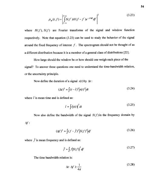
where H(f), S(f) are Fourier transforms <strong>of</strong> the signal and window function<br />
respectively. Note that equation (3.23) can be used to study the behavior <strong>of</strong> the signal<br />
around the fixed frequency <strong>of</strong> interest f . The spectrogram should not be thought <strong>of</strong> as<br />
a different distribution because it is a member <strong>of</strong> a general class <strong>of</strong> distributions [22].<br />
How large should the window be or how should one weigh each piece <strong>of</strong> the<br />
signal To answer these questions one need to understand the time-bandwidth relation,<br />
or the uncertainty principle.<br />
Now define the duration <strong>of</strong> a signal s(t) by At :<br />
where I. is mean time and is defined as:<br />
Now also define the bandwidth <strong>of</strong> the signal S(f) in the frequency domain by<br />
where f is mean frequency and is defined as:<br />
The time bandwidth relation is:<br />
in /1 \


