njit-etd2003-081 - New Jersey Institute of Technology
njit-etd2003-081 - New Jersey Institute of Technology njit-etd2003-081 - New Jersey Institute of Technology
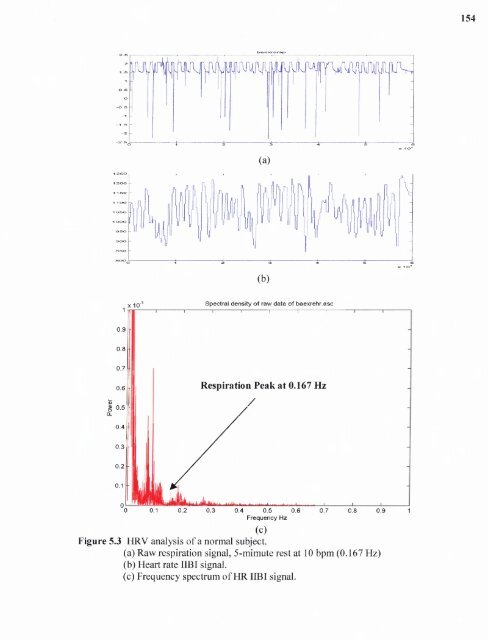
153 Similar spectral analysis is also performed on the heart rate and blood pressure variability signals of a "normal" subject at rest and breathing at 10 bpm (0.167 Hz). The HRV and BPV spectral analysis plots are shown in Figures 5.3 and 5.4. The same strongly influenced respiration frequency peaks of 0.167 Hz can be seen from both the heart rate and blood pressure power spectral density plots of Figures 5.3 and 5.4 (c). As with the COPD subject shown in Figures 5.1 and 5.2, even though the spectral decomposition of both heart rate and blood pressure processes results includes the respiration frequency peaks, each process also exhibits other prominent frequencies, theoretically associated with other physiological processes. The spectral analysis approach, however, has disadvantages. To illustrate this point, the heart rate power spectral density plots and the blood pressure power spectral plots of both the COPD and normal are plotted side by side for comparison, as shown in Figures 5.4.1 and 5.4.2, respectively. Besides some of the obvious differences between the power spectral density plots such as the amplitude of the components at 0.1 Hz, 0.167 Hz, 0.2 Hz, 0.267 Hz, 0.3 Hz and 0.4 Hz etc., there are no other information from these plots that can help to distinguish the COPD subject from the normal subject. These conventional power spectra clearly fail to reflect an appropriate representation of the signal characteristics of the heart rate and blood pressure variability signals. All time information is completely lost; hence there is no way to quantitatively differentiate COPD from normal. Fortunately, there are other techniques such as time-frequency analysis and cross-spectral analysis, which will be presented in later sections, which can overcome these limitations
Figure 5.3 HRV analysis of a normal subject. (a) Raw respiration signal, 5-mimute rest at 10 bpm (0.167 Hz) (b) Heart rate IIBI signal. (c) Frequency spectrum of HR IIBI signal. 154
- Page 131 and 132: 102 variability exists in the propa
- Page 133 and 134: 104 eXogenous input (ARX) was used
- Page 135 and 136: 106 The baroreflex, an autonomic re
- Page 137 and 138: 108 the principal components are no
- Page 139 and 140: 110 The mathematical solution for t
- Page 141 and 142: 112 3.15 Cluster Analysis The term
- Page 143 and 144: 114 formed) one can read off the cr
- Page 145 and 146: 116 3.15.5 Squared Euclidian Distan
- Page 147 and 148: 118 Alternatively, one may use the
- Page 149 and 150: 120 Sneath and Sokal used the abbre
- Page 151 and 152: 122 may seem a bit confusing at fir
- Page 153 and 154: CHAPTER 4 METHODS The purpose of th
- Page 155 and 156: 126 4.1.2.1 Autonomic Testing. HR V
- Page 157 and 158: 128 of heart rate, blood pressure,
- Page 159 and 160: 130 The patients who underwent LVRS
- Page 161 and 162: 132 panel of the Correct.vi. It was
- Page 163 and 164: 134 4.2.3 Power Spectrum Analysis o
- Page 165 and 166: 136 weighted-average value of the c
- Page 167 and 168: 138 For each given scale a within t
- Page 169 and 170: 140 frequency F to the wavelet func
- Page 171 and 172: 142 4.2.8 System Identification Ana
- Page 173 and 174: 144 In this study a simpler approac
- Page 175 and 176: 146 Table 4.2 Parameters That Make
- Page 177 and 178: 148 4.2.11 Cluster Analysis The sam
- Page 179 and 180: 150 viewing the time series of sequ
- Page 181: Figure 5.2 BPV analysis of a COPD s
- Page 185 and 186: Figure 5.4.1 Comparison of the HRV
- Page 187 and 188: 158 5.2 Time Frequency Analysis One
- Page 189 and 190: Figure 5.5 Test signal with 3 sine
- Page 191 and 192: 162 Figure 5.6 (c) CWD of a signal
- Page 193 and 194: 164 Figure 5.7 (c) WT (dB4 wavelet)
- Page 195 and 196: 166 HRV more information about HRV
- Page 197 and 198: 168 Figure 5.9 (c) CWD plots of a n
- Page 199 and 200: Figure 5.10 CWT (Morlet) HRV plot o
- Page 201 and 202: 172 The following figures show the
- Page 203 and 204: 174 Figure 5.15 CWT (Mexican Hat) H
- Page 205 and 206: 176 5.2.5 Best Wavelet Selection fo
- Page 207 and 208: 178 Table 5.1 Correlation Indices o
- Page 209 and 210: 180 5.2.6 Vagal Tone and Sympathova
- Page 211 and 212: 182 These figures basically show th
- Page 213 and 214: 184 Figure 5.20 Sympathetic and par
- Page 215 and 216: 186 Figure 5.24 Sympathetic and par
- Page 217 and 218: 188 5.2.7 Time-Frequency Analysis (
- Page 219 and 220: 190 Figure 5.29 3D and contour plot
- Page 221 and 222: 192 Figure 5.33 3D and contour plot
- Page 223 and 224: 194 Figure 5.34 Sympathetic and par
- Page 225 and 226: 196 Figure 5.38 Sympathetic and par
- Page 227 and 228: 198 Figure 5.42 Sympathetic and par
- Page 229 and 230: Figure 5.44 Plot of raw respiration
- Page 231 and 232: Figure 5.46 The LF partial coherenc
Figure 5.3 HRV analysis <strong>of</strong> a normal subject.<br />
(a) Raw respiration signal, 5-mimute rest at 10 bpm (0.167 Hz)<br />
(b) Heart rate IIBI signal.<br />
(c) Frequency spectrum <strong>of</strong> HR IIBI signal.<br />
154


