Phase transitions of fluids in shear flow

J. Phys.: Condens. Matter 9 (1997) 6119–6157. Printed in the UK PII: S0953-8984(97)66281-5 

REVIEW ARTICLE 

Phase transitions of fluids in shear flow 

Akira Onuki 

Department of Physics, Kyoto University, Kyoto 606, Japan 

Received 14 March 1997 

Abstract. We review theories and experiments on the effects of shear in fluids undergoing 

phase transitions. We put emphasis on near-critical fluids and polymer solutions as representative 

examples, but also discuss related problems in polymer blends, gels, and surfactant systems, 

etc. In near-critical fluids, convective deformations can drastically alter the critical behaviour, 

spinodal decomposition, and nucleation. In this case the hydrodynamic interaction suppresses 

the fluctuations and gives rise to a downward shift of the critical temperature (shear-induced 

mixing). The rheology in two-phase states, and effects of random stirring are also reviewed. 

In semidilute polymer solutions near the coexistence curve, on the other hand, the composition 

fluctuations can be strongly influenced by the viscoelastic stress. In shear flow, this dynamical 

coupling results in enhancement of the composition fluctuations (shear-induced demixing). They 

grow, but are eventually disrupted by convective deformations, yielding chaotic dynamical steady 

states where phase separation is incompletely taking place. Such nonlinear shear regimes are 

examined using computer simulations based on a viscoelastic Ginzburg–Landau model. 

Contents 

1. Introduction 

2. Near-critical fluids under shear 

2.1. The dynamical model 

2.2. The strong-shear regime in one-phase states 

2.3. The shift of the critical temperature 

2.4. Spinodal decomposition in shear 

2.5. Nucleation in shear 

2.6. Rheology in strong shear and in two-phase states 

2.7. Effects of stirring 

3. Shear-induced phase separation 

3.1. Dynamic coupling between stress and diffusion 

3.2. Linear theory for shear flow 

3.3. The normal-stress effect, and the non-Newtonian regime 

3.4. Time-dependent Ginzburg–Landau theory 

3.5. Simulation of shear-induced phase separation 

4. Summary 

Appendices 

1. Introduction 

Flows of fluids are described by a space-time-dependent velocity field. In contrast to solids, 

fluids do not return to their original forms after experiencing shear deformation. The simplest 

example is a plane shear flow whose average profile is 

〈v〉 =Sye x (1.1) 

0953-8984/97/296119+39$19.50 c○ 1997 IOP Publishing Ltd 6119

6120 A Onuki 

with a spatially homogeneous shear rate S. Hereafter the flow direction is taken to be 

along the x-axis, e x being the unit vector along the x-axis, and the mean velocity varies 

in the y- or shear direction, while the z-direction is called the vorticity direction. As is 

well known, if a fixed shear is applied to a fluid of viscosity η, a shear stress σ xy = ηS 

arises. In this typical example of nonequilibrium steady states, the size of S is mostly 

assumed to be much smaller than any underlying relaxation times of the fluid. This is 

the necessary condition for justifying the usual hydrodynamic theory on the basis of the 

local equilibrium approximation. However, in recent years, much attention has come to 

be focused on nonlinear cases, in which a certain internal structure of the fluid is strongly 

affected by the flow field [1–3]. Particularly striking effects arise when shear influences 

phase transitions and phase separation of fluids. Though such effects have been known of in 

polymer science, without satisfactory explanations [4–8], they are becoming very important 

in the study of fluids near the critical point (near-critical fluids) and various complex fluids 

such as polymers, liquid crystals, colloidal systems, and amphiphilic systems. This trend has 

developed out of the foundation of a deep understanding of dynamical critical phenomena 

[9, 10], kinetics of first-order phase transitions [11, 12], and polymer physics [13, 14]. 

Experimentally, this investigation has been accelerated through the recent application of 

scattering techniques to nonequilibrium phenomena under shear. Other optical effects 

such as birefringence and dichroism have also been useful for sensitively detecting spatial 

anisotropy of composition fluctuations, and molecular alignment (see the last paragraph of 

this section). The information gained by these means can then be combined with rheological 

data on the shear stress and normal-stress differences, which in many cases exhibit unusual 

behaviour in nonlinear-response regimes of shear. Though the study of complex fluids under 

shear has often been conducted with the goal of producing engineering-oriented results, it is 

now developing into a new interdisciplinary field, between engineering and physics. Here, 

rheology and phase transitions are closely and uniquely tied. 

Cases in which shear effects are particularly striking and well known include the 

following. 

(1) Fluids with slowly relaxing fluctuations. A representative example here is a fluid 

near its critical point, in which the critical fluctuations are greatly deformed as they are 

convected by a spatially varying velocity field [15–19]. The deformation time is given by 

the inverse shear 1/S, so the deformation is strong or nonlinear when the so-called Deborach 

number De defined by 

De = Sτ ξ (1.2) 

exceeds 1 (the strong-shear case), where τ ξ is the characteristic lifetime of the critical 

fluctuations on the spatial scale of the correlation length ξ and can be measured by means 

of dynamical light scattering. As other conspicuous examples, even not close to critical 

points, entangled polymers [13, 14] and colloidal systems [20–22] exhibit slow stress and 

density relaxations, and are easily driven into nonlinear-response regimes of shear. 

(2) Phase-separating fluids. In a thermodynamically unstable or metastable fluid, twophase 

structures emerge after quenching a fluid. The domain size is small initially and 

grows in time, so the driving force of the instability decreases, and shear can eventually 

suppress the growth, resulting in a dynamically steady, two-phase state. On the other hand, 

nucleation can be suppressed if droplets with the critical size R c are unstable against breakup 

in shear. Furthermore, surfactant molecules, if they are added, tend to be trapped in the 

interface regions, and can stabilize two-phase structures, producing a number of complex 

and intriguing effects on the two-phase domain structure. Shear flow can drastically affect 

phase behaviour of such amphiphilic systems [23–26].

Phase transitions of fluids in shear flow 6121 

(3) Viscoelastic two-component fluids. When the two components have very different 

viscoelastic properties, there arises a dynamical coupling between the stress and diffusion in 

such systems, leading to a number of viscoelastic effects. Among them, shear-induced phase 

separation in semidilute polymer solutions is the most spectacular, and is one of the main 

subjects of this paper. In this case the composition fluctuations produce inhomogeneities 

of stress imbalance resulting in diffusion in the direction of phase separation, giving rise to 

enhanced light scattering even above the coexistence temperature [8]. 

(4) Fluids composed of large (although perhaps simple) constituent elements. In colloidal 

systems, even when a relatively weak experimentally producible shear is applied, the 

structure of the phase can be changed drastically. In particular, shear-induced melting of 

crystal structures has been studied by means of scattering experiments [20–22]. In order to 

produce the same type of change in fluids of small molecules, an unreasonably large shear 

must be used. Moreover, a gas–liquid critical point has recently been found in colloidal 

systems, in which the critical fluctuations are extremely sensitive to shear [27]. 

(5) Fluids with complex internal structure and long-range order. Examples include 

various mesoscopic phases of liquid crystals [28–31], block copolymers [32–36], and 

amphiphilic systems [23–26]. It is obvious that structures such as lamellae or cylinders are 

easily aligned by relatively weak shear. Even their structures and phase behaviour can be 

altered by shear near the transition point. For example, shear can induce transitions between 

phases of lamellae and monodisperse multilamellar vesciles [24] and between isotropic and 

nematic phases giving rise to two-phase coexistence in homogeneous flow [23, 25]. Defects 

can be removed or even generated by shear [37]. We also mention electro-rheological and 

ferromagnetic fluids, in which stringlike structures of colloidal particles are formed due to 

dipolar interaction under an electric or magnetic field. They exhibit unique rheology and 

phase behaviour in shear flow [38, 39]. 

There can be many other cases. Less studied in physics but important in polymer science 

are crystallization [40, 41] and gelation [42, 43] of polymers in a flow field. For highly 

viscous fluids around the glass transition, the structural relaxation time becomes exceedingly 

long, and a marked shear-thinning effect was observed [44]. Very recent molecular dynamics 

simulations on a highly supercooled liquid have reproduced such behaviour [45]. We should 

not forget to mention boundary effects such as the effects of slipping of a viscoelastic fluid 

at a solid boundary [46, 47] or plug flow formation in dense suspensions passing through a 

capillary [48–50]. Furthermore, application of shear to molecular systems inserted between 

two solid plates with spacing of the order of 10 Å has become possible. In such confined 

systems, measurements of the shear stress give information on the shear-induced melting of 

a solid phase and nonlinear rheology of a fluid phase [51, 52]. 

A large number of papers have thus been published on shear flow effects in various 

fluids undergoing some phase transition. It is not easy to cover all of these topics in a single 

review. This is also so because most of them are still developing and not well understood. In 

this article we will focus our attention mainly on near-critical fluids in the above-mentioned 

categories (1) and (2) in section 2, and semidilute polymer solutions in the category (3) in 

section 3. The theoretical foundation of near-critical fluids has no ambiguity, while that of 

polymer solutions has begun to be understood. We will also discuss cases of other fluids as 

much as possible. The approaches here can be starting points for investigating other fluids 

under shear. 

We will thus treat bulk shear effects independent of the distance to the boundary. We are 

above all interested in the structure factor I(q) of the composition fluctuations observable 

by scattering methods. Here we explain why it can be well defined in moving fluids under

6122 A Onuki 

shear flow (1.1), which is not trivial. That is, we show that a sheared fluid still maintains a 

translational invariance in spatial regions far from the boundary, which is an advantage over 

other nonequilibrium situations such as those under a temperature gradient. It follows from 

the fact that a shift of the origin of the reference frame by a along the y-axis is equivalent 

to a Galilean transformation to a new reference frame moving with a velocity −aSe x [15]. 

This implies that, in homogeneous stationary states, the time correlation function of any 

density variable φ(r,t) may be written as 

〈φ(r, t)φ(r ′ ,t ′ )〉=〈φ(r − r ′ − S(t − t ′ )y ′ e x ,t −t ′ )φ(0, 0)〉. (1.3) 

The equal-time correlation function (t = t ′ ) depends only on the relative position r − r ′ . 

Its Fourier transformation yields the steady-state structure factor 

∫ 

I(q) = dr exp[iq · (r − r ′ )]〈φ(r, t)φ(r ′ ,t)〉 (1.4) 

which is observable by means of scattering experiments. Theoretically it goes without 

saying that because of the translational invariance the Fourier transformation may be used 

to greatly simplify the calculations. It is instructive to rewrite (1.3) in terms of the Fourier 

components: 

〈φ q (t)φ k (t ′ )〉=(2π) d δ(q + k + q x S(t − t ′ )e y )I (q,t −t ′ ) (1.5) 

where 

∫ 

I(q,t)= dr exp[iq · r]〈φ(r, t)φ(0, 0)〉. (1.6) 

The first factor in (1.5) is the delta function in d dimensions. To understand its origin 

we note that a plane-wave composition fluctuation (∝ exp(iq · r) at t = 0) with a small 

amplitude changes in time into a plane wave with a time-dependent wave vector given by 

˜q(t) = q − Stq x e y if nonlinear couplings among the fluctuations are neglected. Then (1.6) 

is nonvanishing only for ˜q(−t + t ′ ) =−kon average over the fluctuations, yielding the 

above delta function. It would be informative to measure the time dependence of I(q,t) in 

(1.5), but dynamical light scattering in shear flow has not yet been successful. This seems to 

be because the Doppler shift of scattered light depends on the y-coordinate of the scattering 

position, and the observed signal strongly depends on the thickness of the scattering region 

in the y-direction [53, 54]. 

We also note that anisotropic composition fluctuations in shear flow or electric field 

give rise to anisotropy in the average dielectric tensor at optical frequencies even when 

the constituent particles are optically isotropic [14, 55]. Its real and imaginary parts lead 

to the so-called form birefringence and dichroism, respectively. In particular, the form 

dichroism is significant when the spatial scales of scattering objects are comparable to the 

light wavelength. This effect has been measured in near-critical fluids [56] and polymeric 

systems [57] in shear flow. On the other hand, alignment of optically anisotropic molecules 

in the external field gives rise to the so-called intrinsic birefringence, whereas the intrinsic 

dichroism is negligible for visible light in most cases. 

2. Near-critical fluids under shear 

In this section we will mainly consider near-critical fluids in which the critical fluctuations 

are important. However, readers need not be unduly concerned with the mathematical 

details of the theory. We start with mean-field calculations, and take into account 

the renormalization effects in the simplest manner. Shear effects arise solely from


position-dependent convection or convective deformations of the composition fluctuations. 

Nevertheless, the effects are very complex and even surprising, particularly in spinodal 

decomposition and nucleation. We will also discuss the effects of stirring on the critical 

behaviour and phase separation of fluids, which experimentalists have been interested in but 

have not yet well understood. 

2.1. The dynamical model 

In near-critical fluids, a scalar order parameter ψ(r,t) exhibits enormous thermal 

fluctuations on approaching the critical point [9, 10]. We will call this the composition, 

supposing a fluid binary mixture near the consolute critical point with a weak singularity 

of the isothermal compressibility. While its local variations remain small, its spatial 

correlations extend over a long distance ξ, which is the origin of various critical singularities. 

This length is called the correlation length, and grows as ξ = ξ 0 (T /T c − 1) −ν as T → T c 

at the critical value of the average composition, ξ 0 being a microscopic length (∼2 Å) and 

ν ∼ = 0.625 being the critical exponent. 

The Ginzburg–Landau–Wilson free-energy functional for ψ is written in the usual 

form [10]: 

∫ [ 1 

F = k B T c dr 

2 r 0ψ 2 + 1 4 u 0ψ 4 − hψ + 1 ] 

2 C 0|∇ψ| 2 . (2.1) 

Here r 0 is the mean-field reduced temperature, and u 0 is the nonlinear coupling coefficient. 

h, which corresponds to a magnetic field in Ising spin systems, almost vanishes at the critical 

composition above T c and on the coexistence curve. The coefficient C 0 will be set equal to 

1 because it is almost unchanged even after the renormalization. The dynamical equations 

for ψ and the velocity field deviation v are given by [15] 

∂ ∂ψ 

ψ =−Sy 

∂t ∂x − ∇·(ψv) + (L 0/k B T c )∇ 2δF 

δψ + θ R (2.2) 

¯ρ ∂ ∂t v =−∇p 1−ψ∇ δF 

δψ + η 0 ∇ 2 v + ζ R . (2.3) 

The mass density ¯ρ is assumed to be a constant. It is known that slow motion of ψ is not 

affected by the longitudinal part of v, so we are allowed to consider the transverse part 

only: 

∇·v=0. (2.4) 

The pressure p 1 in (2.2) is determined to ensure this condition. θ R and ζ R are Gaussian– 

Markovian thermal noises related to the kinetic coefficients L 0 and η 0 by 

〈θ R (r,t)θ R (r ′ ,t ′ )〉=−2L 0 ∇ 2 δ(r − r ′ )δ(t − t ′ ). (2.5) 

〈ζ Ri (r,t)ζ Rj (r ′ ,t ′ )〉=−2k B Tη 0 δ ij ∇ 2 δ(r − r ′ )δ(t − t ′ ). (2.6) 

Furthermore, because the timescale of v is much shorter than that of ψ, we may set 

∂v/∂t = 0 in (2.3) as a very good approximation, and may express v as [58] 

[ 

−η 0 ∇ 2 v = − ψ ∇ δ ] 

δψ F + ζ R 

(2.7) 

⊥ 

where [···] ⊥ denotes taking the transverse part (perpendicular to the wave vector q in the 

Fourier space). The same approximation is widely used also for colloidal systems (the 

Stokes approximation).

6124 A Onuki 

In renormalization group theory we decrease the upper cut-off wavenumber of the 

fluctuations by averaging over the small-scale fluctuations, and examine how the coefficients 

in the dynamical model (as well as those in the free energy F ) are changed or renormalized 

[10]. Systematic analysis is possible here if use is made of the expansion in ɛ = 4 − d. In 

our model the following static and dynamical quantities tend to universal numbers: 

g 0 = K d u 0 / ɛ → 2 ɛ +··· (2.8) 

3 

f 0 = K d k B T c /L 0 η 0 ɛ → 24 ɛ +··· (2.9) 

19 

where the coefficients are functions of , and K d = (2π) −d 2π d/2 / Ɣ(d/2). If the fluid is 

sufficiently close to the critical point, the above limits are attained even for ≫ ξ −1 , and 

the nonclassical critical behaviour follows. Then the renormalized coefficients are obtained 

at = ξ −1 because the fluctuation effects are weak for 1. Hereafter we are interested in the strong-shear 

regime, Sτ ξ > 1, in which the critical fluctuations are drastically altered by shear before 

they dissipate thermally. It is convenient to introduce a characteristic wavenumber k c via 

Ɣ(k c ) = S. Using (2.12) we obtain 

k c = (6πη/k B T) 1/3 S 1/3 . (2.13)


Then, by setting k c ξ = k c ξ 0 τs 

−ν , we may introduce a crossover reduced temperature τ s as 

follows [19, 59]: 

τ s = (6πηξ0 3 /k BT) 1/3ν S 1/3ν ∝S 0.54 . (2.14) 

Slightly different definitions of k c and τ s follow if use is made of the dynamical 

renormalization group theory. The critical fluctuations are strongly deformed by shear 

in the long-wavelength region q 0. We start with the 

mean-field approximation or linearizing the dynamical equation (2.2). In the Fourier space 

it reads 

∂ 

∂t ψ ∂ 

q = Sq x ψ q − L 0 q 2 (r 0 + q 2 )ψ q + θ Rq . (2.15) 

∂q y 

The fluctuations are simultaneously convected by shear, and thermally dissipated with the 

decay rate (in the mean-field theory) given by 

Ɣ(q) = L 0 q 2 (r 0 + q 2 ). (2.16) 

The steady-state structure factor I(q) satisfies 

[ 

] 

∂ 

2Ɣ(q) − Sq x I(q) = 2L 0 q 2 . (2.17) 

∂q y 

The right-hand side arises from the thermal noise term θ Rq (t), giving rise to the Ornstein– 

Zernike form I OZ (q) = 1/[r 0 + q 2 ] without shear. The simplest way to examine the shear 

effect is to expand I(q) in powers of S as follows: 

I(q)/I OZ (q) = 1 − 2q x q y I OZ (q)S/ Ɣ(q) +···. (2.18) 

Thus the intensity increases most in the directions in which q x =−q y in the q x –q y plane. 

Certainly, the shear effect becomes important when the (mean-field) strong-shear condition 

S>L 0 r0 2 holds. Generally, taking into account the convection due to shear, we may solve 

(2.17) in the following integral form: 

I(q) = 

∫ ∞ 

0 

dt exp 

[ 

− 2 

∫ t 

0 

] 

dt 1 Ɣ(|q(t 1 )|) 2L 0 q(t) 2 (2.19) 

in terms of a deformed wave vector defined by 

q(t) = q + Stq x e y (2.20) 

which is equal to ˜q(−t) introduced below (1.6). Because (2.19) is complex, we give an 

approximate expression interpolating between various limiting cases of (2.19): 

I(q) ∼ = 1/[r 0 +ckc 8/5 |q x | 2/5 + q 2 ] (2.21) 

where c ∼ 1, and k c is determined by L 0 kc 

4 = S in the mean-field theory. Notice that 

I(q) ∼ kc 

−8/5 |q x | −2/5 for most of the wave vectors smaller than k c in strong shear (which 

means r 0

6126 A Onuki 

contributions is k c in strong shear, while it is ξ −1 near equilibrium. For example, the 

renormalized kinetic coefficient in strong shear is 

L = k B T/6πηk c ∝ S −1/3 . (2.22) 

Obviously, if k c is replaced by ξ −1 , the renormalized kinetic coefficient near equilibrium is 

obtained. The structure factor after the renormalization is roughly of the form 

I(q) ∼ = 1/[A(T − T c (S)) + ckc 8/5 |q x | 2/5 + q 2 ] (2.23) 

with 

A = ξ −2 

0 

τs 2ν−1 /T c (2.24) 

where k c and τ s are defined by (2.13) and (2.14). Again, if τ s in equation (2.24) is 

replaced by (T − T c )/T c and the limit S → 0 is taken, we obtain the equilibrium result 

A(T − T c ) → ξ −2 . 

In near-critical fluids, the statical and dynamical renormalization effects are crucial, 

leading to (2.22) and (2.23). There are also systems in which the renormalization effects 

are negligible. As an extreme example, Dhont and Verduin [27] have examined shear effects 

in near-critical colloidal systems with attractive interaction superposed onto the hard-core 

repulsion, in which ξ 0 = 2000 Å and the mean-field theory holds. 

2.3. The shift of the critical temperature 

Next we discuss the critical temperature T c (S) in shear flow. We define the inverse susceptibility 

r = 1/I (q) in the limit where q x = 0 and q → 0. It vanishes at T = T c (S), and 

differs from the coefficient r 0 in F given in (2.1). The difference r = r − r 0 arises first 

from the quartic term in F as follows: 

(r) s = 1 ∫ 

2 u 0 

q 

1 

q 2 + 1 2 u 0 

∫ 

q 

(I(q)− 1 q 2 ) 

+··· (2.25) 

and secondly from the hydrodynamic interaction as follows: 

( 

(r) h = 1 − 1 ) 

∫ 

1 

(k B T c /η 0 L 0 ) 

d 

q q (1 − 2 q2 I(q)) +··· (2.26) 

where ∫ q (···) = ∫ (2π)−d dq (···), and I(q) is the structure factor at the critical point. 

We may derive (2.26) readily from the Kawasaki expression (2.7). Because shear flow 

suppresses the fluctuations, the second term of (r) s is negative and (r) h is positive, 

while they vanish in equilibrium. 

In our original theory [15], we considered low-molecular-weight fluids, and calculated 

the shift of T c assuming that the asymptotic limits (2.8) and (2.9) are attained for much 

larger than k c . Let us explain our result in this case using the ɛ-expansion. We note that 

the dominant contributions in the last two integrals of (2.25) and (2.26) arise from q ∼ k c , 

so by using (2.8) and (2.9) at a value of ∼ k c we obtain 

(r) s = 1 ∫ 

2 u 0 

q 

1 

q 2 − 0.0442 ɛk2 c (2.27) 

(r) h = 0.1274 ɛk 2 c . (2.28) 

Using (2.23) and (2.24) and summing these two contributions, we obtain 

(T c (S) − T c (0))/T c = (0.0442 − 0.1274)ɛτ s =−0.0832 ɛτ s (2.29a)


where τ s is defined by (2.14). In three dimensions we expect 

(T c (S) − T c (0))/T c ∼−0.1τ s . (2.29b) 

The equilibrium critical temperature T c (0) is already shifted downwards from the mean-field 

critical temperature, which is simply the first term of (2.25) for small u 0 . Shear suppresses 

the critical fluctuations and reduces this contribution, giving rise to the second term of (2.25). 

The nonlinear hydrodynamic interaction accelerates the diffusive decay of the fluctuations, 

leading to a larger downward shift of T c . 

Beysens et al detected a downward shift from the turbidity and the structure factor, 

with q perpendicular to the flow. It was proportional to S 0.53 , but four times smaller than 

the result (2.29) at ɛ = 1 in a few critical binary mixtures [18], so this aspect remains 

undecided. We note that it is difficult to determine the small shift definitively in usual 

binary mixtures, because the scattering is suppressed even at T = T c (S) as shown in (2.23), 

and does not grow indefinitely below T c (S) due to formation of stringlike domains, as will 

be explained in the next subsection. 

Hashimoto et al [61–67] used a ternary mixture of polystyrene (PS) and polybutadiene 

(PB) in a common solvent of dioctylphthalate (DOP) to find a downward shift (T c (S) − 

T c (0))/T c ∼ A c τ s with τ s ∝ S 0.5 and A c 

∼ = 0.06 [62]. That is, the scattering intensity above 

T c (S) perpendicular to the flow (q x = 0) was expressed as 

1/I (q) ∼ = ξ −2 

0 

(T − T c (0))/T c + A c kc 2 + q2 . (2.30) 

The second term gives rise to the downward shift. On the other hand, shear-induced 

homogenization took place at the same condition T = T c (S) if shear was increased from 

two-phase states at fixed T below T c (0). In their system the polymer volume fraction 

φ = φ PS +φ PB is of the order of the overlapping value, and the fluid may be treated as 

a binary mixture of weakly interacting PS-rich blobs and PB-rich blobs [67]. The space 

scale and timescale are much more enlarged than for usual binary mixtures, as τ ξ ∼ 1s 

even for T − T c ∼ 10 K and ξ 0 ∼ 50 Å. The crossover reduced temperature τ s in (2.14) is 

three or four orders of magnitude larger than for usual binary mixtures. In the temperature 

region investigated, the static properties are described by mean-field theory, whereas the 

diffusion constant D mol = L 0 |r 0 | of molecular origin and that, D hyd = k B T/6πηξ, from the 

hydrodynamic interaction are not very different, as D hyd /D mol ∼ 0.2–0.5 [62]. We believe 

that the observed downward shift should be due to the hydrodynamic interaction, which 

is consistent with (2.26). Very recently Yu et al [68] have used fluorescence and phasecontrast 

microscopy on a similar ternary mixture of PS + PB in DOP, and have reported 

that the shift tends to saturate at very high shear. 

We note that the shift (2.29) is calculated on the rather special assumption of the 

asymptotic limits (2.8) and (2.9). However, they may not be satisfied in polymeric fluids, 

on which a number of shear flow experiments have been performed. We need to know the 

details of the critical fluctuations, the relevance of the hydrodynamic interaction, and the 

degree of viscoelasticity to reliably estimate the shift of the critical temperature. Polymer 

blends should exhibit complicated crossover effects in shear, depending on the distance to 

the critical point and the molecular weights, etc (where complexity is further increased in 

the presence of large asymmetry between the two components) [69–72]. 

Here, we also make a comment on the shear-induced shift of the transition temperature 

in the microphase separation in diblock copolymers. In such systems the structure factor has 

a maximum at an intermediate wavenumber q m , and the nonlinear hydrodynamic interaction 

is not relevant [33]. Cates and Milner [34] calculated an upward shift from (2.25) using 

the bare u 0 , neglecting the renormalization effect and the hydrodynamic interaction. Their 

prediction was in qualitative agreement with subsequent scattering experiments [35].

6128 A Onuki 

2.4. Spinodal decomposition in shear 

More dramatic are the effects of shear in the unstable temperature and composition region. 

This problem is of technological importance in polymer systems. Beysens and Perrot 

performed a spinodal decomposition experiment on a near-critical binary mixture below 

T c by periodically tilting a quartz pipe container [73]. Such a periodic shear was found 

to prevent the development of decomposition, resulting in a permanent spinodal ring of 

the scattered light. For steady shear, it was anticipated that domains are elongated in the 

flow direction as Stξ in an initial stage [74], which was in agreement with a subsequent 

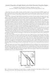
light scattering experiment [19]. In figure 1 we show light scattering patterns obtained 

from a phase-separating fluid in shear, which are characterized by strong anisotropy (streak 

patterns) even in weak shear, Sτ ξ ≪ 1, below T c [19, 59]. Computer simulations in two 

dimensions have also shown strong deformations of bicontinuous domain structures just 

after quenching [75–79]. Moreover, it has also been observed that spinodal decomposition 

is stopped in steady shear at a particular stage [61, 62], giving rise to dynamical stationary 

states. Such sates can be realized only by balance of the two competing mechanisms of 

thermodynamic instability and flow-induced deformation. In these two-phase states we may 

neglect the gravity effect when the domain size R is very small (as compared to the so-called 

capillary length). The Reynolds number Re of a domain is given by Re = ρSR 2 /η, and is 

very small near the critical point [16]. (Far from the critical point we may well encounter 

the opposite limit Re ≫ 1, where the effect of inertia is crucial [16, 80].) 

Figure 1. The time evolution of light scattering patterns from a phase-separating near-critical 

binary mixture at the critical composition [19]. Here S = 0.035 s −1 and T c − T ∼ 1 mK, so 

Sτ ξ ∼ 0.01. The upper patterns (A) are those in the q x –q y plane, while the lower ones (B) are 

those in the q x –q z plane. 

Unfortunately, detailed information cannot be gained from scattering alone, so some 

theoretical speculations were advanced regarding the domain morphology giving rise to 

streak patterns [81]. Recently Hashimoto et al [82] have taken microscope pictures of a DOP 

solution mentioned in subsection 2.3 to investigate the ultimate bicontinuous morphology 

in shear in real space as shown in figure 2. They have found that domains are elongated 

into extremely long cylinders in steady states except for in the case of extremely weak 

shear. For Sτ ξ < 1, such stringlike domains still contain a number of random irregularities 

undergoing frequent break-up, interconnection, and branching, although the overall structure 

is kept stationary. For Sτ ξ > 1 the continuity of the strings increases, and extends even 

macroscopically in the flow direction. The scattering intensity perpendicular to the flow is


Figure 2. Microscope images ((a), (c), (e)) and corresponding light scattering patterns ((b), 

(d), (f )) for a PS/PB(80:20)/DOP 3.3 wt% solution at T c − T = 10 K (taken by Hashimoto’s 

group). Here (a) and (b) were obtained under steady shear at 4 s −1 , while (c) to (f ) were obtained 

at 90 s and 250 s after cessation of the shear. We can see break-up of cylindrical domains into 

droplets, which occurs on the timescale of ηξ ⊥ /σ , where σ is the surface tension and ξ ⊥ is the 

cylinder diameter. 

proportional to the squared Lorentzian form 1/[1 + (qξ ⊥ ) 2 ] 2 due to cylindrical domains, 

where ξ ⊥ represents the diameter of the cylinders, and decreases with shear as 

ξ ⊥ 

∼ = [10/qm (0)](Sτ ξ ) −α (2.31)

6130 A Onuki 

where q m (0) is the peak wavenumber in spinodal decomposition without shear, and 

α = 1/4 − 1/3. For very large shear S 10 2 /τ ξ , the diameter ultimately becomes of the 

order of the interface thickness, and the contrast between the two phases vanishes, resulting 

in shear-induced homogenization (at T = T c (S) for the case at the critical composition). 

Very recently, Hobbie et al [83] studied the dynamics of the formation of the string 

phase in a DOP solution after application of shear. Also, for usual binary mixtures, Hamano 

has observed extreme elongation of domains in strong shear Sτ ξ 1 [84]. Note that the 

streak scattering patterns in DOP solutions closely resemble those in usual binary mixtures 

[19, 59]. We should also mention that microscope pictures of stringlike domains were 

reported for polymer blends [85]. 

We note that the surface tension is extremely small ( 10 −4 cgs) in Hashimoto’s 

case and those of usual binary mixtures. We believe that shear can suppress surface 

undulations of cylindrical domains for very low surface tension. Such undulations grow, 

resulting in break-up of cylinders into droplets in the absence of shear (the Tomotika 

instability [86]). Figure 2 shows a dramatic example observed after cessation of the shear. 

Interestingly, this capillary-driven instability is in essence the coarsening mechanism of latestage 

spinodal decomposition at the critical composition [87]. Rheologically, there should 

be no appreciable increase η of the macroscopic viscosity in the string phase, where the 

surfaces do not resist the flow. This point will be discussed again in subsection 2.6. 

Very recently, spinodal decomposition under shear flow has been studied by molecular 

dynamics (MD) simulation of a two-dimensional Lennard-Jones system consisting of 40 000 

particles [79]. This has involved applying a very large shear realizable only in MD 

simulations, and examination of elongated domain morphologies below T c . We notice 

that the simulation [79] has been performed in a regime with a relatively large Reynolds 

number, Re = ρSR 2 /η 1, with significant velocity field fluctuations. 

We may also consider spinodal decomposition under oscillating shear, S(t) = S 0 cos(ωt). 

Krall et al [88] pointed out a new bifurcation effect under periodic shear on the basis of a 

phenomenological domain growth theory of Doi and Ohta [89]. That is, if the maximum 

shear strain f = S 0 /ω is larger than a critical value f c , the shear distortion is effective 

enough, and the domain growth can be stopped, resulting in a periodic two-phase state. 

If f < f c , the shear cannot stop the growth leading to macroscopic phase separation. 

Interestingly, a similar bifurcation was found in a spinodal decomposition experiment under 

periodic quenching [90]. 

2.5. Nucleation in shear 

2.5.1. Droplet break-up and coagulation in shear. We then slightly lower the temperature 

T below the coexistence temperature T cx by δT = T cx − T in the off-critical case. To 

observe appreciable droplets of the new phase, the critical droplet must not be torn by 

shear, and hence we require 

R c


This gives an upper limit for the shear, S ∗ ∼ /τ, at each δT , or a lower limit for the 

quench depth 

δT ∗ ∼ Sτ(T ) ∝ S(T ) 1−3ν (2.35) 

at each S, in order to have droplets. This simple criterion has been confirmed for binary 

mixtures under gentle stirring [95, 96] and uniform shear [97]. 

The key quantity in the initial stage of nucleation is the nucleation rate [11, 12] 

J ∝ exp(−a(T /δT ) 2 ) (2.36) 

where a is a number of order 1. It is the probability of finding droplets with radius larger 

than R c per unit volume and per unit time. It is known that J can be of order 1 when δT 

is equal to the classical Becker–Döring limit 

δT BD 

∼ = 0.15 T . (2.37) 

We note that δT ∗

6132 A Onuki 

of order 1/φS (the mean free time) where φ is the droplet volume fraction. This estimation 

is valid when the sizes of the colliding droplets are of the same order. On the other hand, 

flow-induced collisions rarely occur between droplets with very different sizes, because the 

smaller one moves on the stream line of the velocity field around the larger one without 

appreciable diffusive motion for Pe ≫ 1 [100, 101]. Due to this coagulation, the average 

droplet size grows as [99, 102] 

( ) ∂R 

∼ SφR (2.38) 

∂t coll 

leading to an exponential growth of R. 

For aggregating colloidal systems, the above exponential growth is well known [102]. 

Simulations of colloid aggregates have shown deformation, rupture, and coagulation of 

clusters in shear flow [103, 104]. These hydrodynamic effects are of great technological 

importance for two-phase polymers [105], in particular in the presence of copolymers [106]. 

Here we raise a fundamental question as to the existence of metastability itself in 

relatively large shear for which (2.34) is not satisfied. That is, if δT is increased in 

such shear, droplet formation will be suppressed, because localized droplets larger than 

R ∗ cannot be stable. In particular, if Sτ ξ ∼ 1, R c becomes of order ξ and the suppression 

is complete, in the sense that phase separation can be triggered only by instability of planewave 

fluctuations. That is, a spinodal point becomes well defined in such relatively large 

shear as the unique onset point of phase separation. Recall that the spinodal point obtained 

in the mean-field theory has no definite theoretical meaning for quiescent fluids [11, 12]. 

2.5.2. Droplet size distribution in shear. Under (2.34), a nearly stationary distribution of 

droplets is realized after a long relaxation time [97]. Remarkably, the size distribution is 

peaked at R ∼ = R ∗ and, once such a distribution is established, further time development of 

the droplet distribution becomes extremely slow. Min and Goldburg [97] have found that the 

supersaturation tends to a finite value (S) dependent on S by gradually increasing δT 

from zero, which corresponds to the branch H in figure 3. It can be determined because the 

droplet volume fraction is φ = (0) −(S). Though such a state is nearly stationary, there 

is still a diffusive current onto each droplet from the surrounding metastable region. Each 

droplet will grow above R c and break into smaller droplets, which will then start to grow 

again or dissolve into the metastable region depending on whether their radii are larger or 

smaller than R c . Each droplet will also collide with another one on the timescale of 1/Sφ. 

The evolution of the droplet size distribution is therefore very complex, and the observed 

quasi-stationarity is produced by a delicate balance among these processes. Alternatively, 

we may also start with an opaque state in which δT is sufficiently large and (S) ∼ = 0 (or 

φ ∼ = (0)). Then, by gradually decreasing δT at fixed S, a nearly stationary state will be 

obtained, which corresponds to the branch C in figure 3. Interestingly, it has been found to 

be more opaque and to have a larger droplet volume fraction (or a smaller supersaturation) 

than in the reverse case of increasing δT from zero. 

Hashimoto et al [65, 66] have observed similar hysteresis in off-critical DOP solutions 

by increasing or decreasing S over a very wide range with δT fixed. First, they increased 

S from an opaque state with droplets to reach a transparent state without droplets at 

T spi (0) − T ∝ S, where T spi (0) is the cloud-point temperature at zero shear. We believe that 

this disappearance of droplets should have been caused by the Taylor break-up mechanism, 

though the difference between T spi (0) and the temperature T cx on the coexistence curve is 

not clarified in their work. Second, they decreased S from a disordered state homogenized 

by large shear to reach a spinodal-like point at which T spi (0) − T ∝ S 1/2 , and below which


droplets appear. However, they found that the quasi-steady states reached in the decreasing 

branch are still slowly evolving towards the steady states reached in the increasing branch 

on timescales of several hours. We believe that the experiments performed by Hashimoto 

et al and those performed by Goldburg and Min are consistent with each other. 

2.5.3. Acceleration of droplet growth in shear. To analyse their experiment, Baumberger 

et al [107] argued that the growth of an isolated droplet in a metastable fluid can be 

considerably accelerated even in very weak shear by an advection mechanism. If the growth 

is slow, the composition ψ outside the droplet is determined by a quasi-static condition: 

u ·∇ψ+D∇ 2 ψ =0 (2.39) 

where u is the average flow tending to a simple shear flow far from the droplet. The relative 

importance of the two terms in (2.39) is given by the Peclet number 

Pe = SR 2 /D = Sτ ξ (R/ξ) 2 . (2.40) 

We have Pe > Sτ ξ / 2 for R>R c , and Pe ∼ 1/St ξ at the break-up size R ∼ R ∗ . Thus 

Pe ≫ 1 can hold over a sizable time interval even under (2.32) or (2.34). The deviation 

from the spherical shape is small for R ≪ σ/ηS or for R ≪ R ∗ . For Pe ≫ 1 it is important 

that the composition gradient is localized in a thin layer, with a thickness l S given by 

l S ∼ (D/S) 1/2 ∼ R/ √ Pe (2.41) 

around the droplet. This relation follows from the balance between the two terms in (2.39). 

As a result, the diffusion current onto the droplet from the metastable fluid is enlarged by 

l S /R ∼ Pe 1/2 as compared to the case where Pe ≪ 1 [108, 109], so the usual Lifshitz– 

Slyozov equation [110] is modified as follows: 

∂ 

∂t R ∼ D R 

( 

− 2α R 

)Pe 1/2 ∼ (SD) 1/2 ( 

− 2α R 

) 

(2.42) 

where α is a capillary length (∼ξ). Thus the timescale of the initial stage can be considerably 

accelerated by the convection effect. However, the critical radius R c = 2α/ is unchanged 

by very weak shear, and there seems to be no drastic change in the nucleation rate, although 

this is not confirmed. 

The above mechanism is important in systems with a small diffusion constant such 

as polymer blends. As another similar effect we note that, if surfactant molecules are 

added to an oil–water two-phase system, they can be advected onto the oil–water interfaces 

efficiently in shear flow, leading to shear-induced emulsification. Systematic experiments 

in these cases should be interesting. 

2.6. Rheology in strong shear and in two-phase states 

The fluctuations of the order parameter ψ give rise to the following additional shear stress 

[114, 113]: 

Sη=−k B T〈(∂ψ/∂x)(∂ψ/∂y)〉 (2.43) 

where the average is taken in a system under shear. Other important quantities include the 

normal-stress differences: 

N 1 = σ xx − σ yy = k B T 〈(∂ψ/∂x) 2 − (∂ψ/∂y) 2 〉 (2.44) 

N 2 = σ yy − σ zz = k B T 〈(∂ψ/∂y) 2 − (∂ψ/∂z) 2 〉. (2.45)

6134 A Onuki 

In the one-phase region, the above quantities may be expressed as integrals in the wavevector 

space using the structure factor I(q). We find that η is nearly logarithmic, varying 

as log(ξ/ξ 0 ) in weak shear and as log(1/k c ξ 0 ) in strong shear. This crossover was first 

predicted by Oxtoby [111]. If use is made of the ɛ-expansion in strong shear, we obtain 

[112] 

η = η 0 + η ∝ (k c ξ 0 ) −x η 

∝ S −x η/d 

(2.46) 

where x η = ɛ/19 + ··· is a small dynamical exponent. This shear rate dependence 

was measured by Hamano et al [115]. In weak shear, the normal-stress differences are 

proportional to S 2 and are very small. In strong shear, the wave-vector integrals in (2.43)– 

(2.45) are of order ηkc d, and 

N 1 = 0.046ɛηS N 2 =−0.032ɛηS (2.47) 

to first order in ɛ. (Note that N 1 and N 2 are even functions of S, while the shear stress σ xy 

is odd. If we allow the case where S


scattering pattern emerges with η(t) → 0, we may conclude that a string phase discussed 

in subsection 2 was realized in their critical quench cases. For such highly elongated 

domains, the interfaces are mostly parallel to the flow, and n x 

∼ = 0 in (2.48), leading to 

η ∼ = 0. 

Recently, the rheology of phase-separating polymer blends has also been studied [120– 

122] particularly when the two phases are Newtonian and have almost the same viscosity. 

The observed η and N 1 were in excellent agreement with the scaling relations (2.50) and 

(2.51). It is of great importance in polymer physics to understand the rheology in more 

complex two-phase states, such as in the case in which the viscosity difference between the 

two phases is large [118, 123], or the case in which viscoelasticity is crucial. The latter 

case will be discussed in subsection 3.5. 

In aqueous surfactant solutions, marked increases of the viscosity and N 1 were observed, 

which was interpreted as arising from shear-induced aggregate formation or gelation [42]. 

In aqueous solutions of agarose, huge viscosity enhancement was also observed, in which 

gelation was probably induced upon phase separation [124]. In colloids near the critical 

point [125] and dense microemulsions near the percolation threshold [126], the viscosity 

has been reported to grow strongly, in contrast to the weak-viscosity singularity in the usual 

near-critical fluids. In such systems, near a phase transition, interesting nonlinear rheology 

might well be expected at high shear and/or in two-phase cases. 

Simulations of simple fluids in two dimensions have also shown an increase of the 

viscosity in spinodal decomposition [75–77, 79]. In the MD study of a Lennard-Jones 

fluid [79], dynamical steady states with irregularly elongated domains have been attained. 

Simulations of fluids with internal structures in this direction should be of great importance. 

(An example for the viscoelastic case will be given at the end of section 3.) 

2.7. Effects of stirring 

Fluids can be mixed even by gentle stirring, so it is always used in experiments and in 

everyday life. Voronel and co-workers [127] measured the specific heat C v under stirring 

in one-component fluids near the gas–liquid critical point. Surprisingly, they could observe 

a sharp peak of C v even very close to the critical point, which would have been masked 

by the gravity effect in a quiescent fluid. To support their finding, we may argue [128] that 

the density stratification in gravity is much reduced from −ρg(∂ρ/∂p) T to −ρg(∂ρ/∂p) s 

under stirring. The ratio of these two quantities is (∂ρ/∂p) T /(∂ρ/∂p) s = C p /C v , and is 

very large near the gas–liquid critical point. This means that the entropy per unit mass s 

tends to be homogenized in stirred fluids despite the presence of a pressure gradient. There 

should also arise a vertical temperature gradient 

dT/dz =−ρg(∂T /∂p) s (2.52) 

which is −0.9 mK cm −1 on earth in xenon. Also, in binary mixtures, if use is made of the 

derivative (∂T /∂p) sX at fixed composition X, we can predict the same temperature gradient. 

Cannell [129] first reported the presence of a temperature nonuniformity in stirred fluids in 

gravity. But there has been no systematic experiment to confirm the above predictions. 

We may also examine critical phenomena and phase separation of near-critical binary 

mixtures in vigorous stirring or turbulence [130–133]. It is known that the maximum shear 

rate S d in turbulence is given by (η/ρ)kd 2, where 

k d = L −1 

0 Re3/4 (2.53) 

is the Kolmogorov lower cut-off wavenumber, L 0 being the size of the largest eddies and 

Re being the Reynolds number, much larger than 1. We note that in the case of near-critical

6136 A Onuki 

fluids, the composition fluctuations have sizes much shorter than the size of the smallest 

eddies (∼1/k d ), and are most effectively strained by the smallest eddies. These eddies turn 

over on the timescale of 1/S d , during which the composition fluctuations are affected by 

the eddies. Experiments showed that there is no sharp phase transition in turbulence, and 

that the scattered light intensity increases gradually but dramatically as T is lowered below 

T c . As in the case of laminar shear, there is a strong-shear regime determined by τ ξ S d > 1, 

in which the fluctuations are strongly suppressed by random shear. If a fluid is further 

quenched below T c into the weak-shear region τ ξ S d ≪ 1, the characteristic domain size 

should be given by 

R ∼ σ/ηS d ∼ (ρσ/η 2 )k −2 

d 

(2.54) 

as for laminar shear [16]. Note that the above scenario holds only for R


dynamical coupling mechanism first applied to sheared polymer solutions by Helfand and 

Fredrickson [149, 153], (ii) a viscoelastic Ginzburg–Landau scheme [150, 151, 154, 155] 

with a conformation tensor as a new independent dynamical variable, and (iii) computer 

simulations [156] which would give insights into strongly fluctuating polymer solutions 

under shear. However, a number of puzzles remain unexplored in spinodal decomposition 

and nucleation with (and even without) shear below the coexistence curve. 

We should also mention intriguing small-angle neutron scattering experiments on gels 

which are swollen and uniaxially expanded [157]. Heterogeneities of the crosslink structure 

are believed to induce frozen composition variations giving rise to abnormal butterfly 

scattering patterns [157–160], which are very similar to those from sheared polymer 

solutions in the q x –q z plane [143, 147, 159]. For both polymer solutions and gels, the 

problems encountered are those of the stress balance attained by composition changes in 

heterogeneous systems. The difference is that the crosslink structure is permanent in gels 

and transient in polymer solutions, which makes the problem simpler (though still complex) 

for gels [159]. 

3.1. Dynamical coupling between stress and diffusion 

Semidilute polymer solutions become highly viscoelastic when the molecular weight is 

very large and when the polymer volume fraction φ exceeds the critical volume fraction 

φ c = N −1/2 , where N is the polymerization index (the number of segments on a chain), 

much larger than 1. We assume that the polymer volume fraction φ is much smaller 

than 1, and will replace the factor 1 − φ by 1 in many relations to follow. The viscosity 

η and the stress relaxation time τ dramatically increase with increasing φ and N, because 

a large network stress is produced due to entanglement even against small deformations. 

It has recently been recognized that the stress can influence spatial inhomogeneities of the 

composition through a dynamical coupling between stress and diffusion. This coupling 

gives rise to nonexponential relaxation of the time correlation function of the composition 

fluctuations near equilibrium [161–165]. 

To illustrate this new concept, let us consider a simple two-fluid model of polymer 

solutions [149–156, 166, 167]. The mass densities, ρ p and ρ s , of the polymer and the 

solvent are convected by their velocities, v p and v s , as follows: 

∂ 

∂t ρ ∂ 

p =−∇·(ρ p v p ) 

∂t ρ s =−∇·(ρ s v s ). (3.1) 

The total density ρ = ρ p + ρ s obeys the usual continuity equation with the momentum 

current ρv, where the average velocity v is defined by 

v = ρ −1 (ρ p v p + ρ s v s ). (3.2) 

Most polymer solutions have a very small compressibility or are nearly incompressible. 

Therefore the density deviation δρ = ρ − ¯ρ from the average ¯ρ is very small, and the 

continuity equation may be linearized as 

∂ 

δρ =−¯ρ∇·v. (3.3) 

∂t 

For simplicity, we further assume that the mass densities of pure polymer and solvent are 

the same. Then the mass fraction ρ 1 /ρ coincides with φ. It obeys 

( ) 

∂ 

∂t + v ·∇ φ=−∇·(φ(1 − φ)w) ∼ = −∇·(φw) (3.4)

6138 A Onuki 

where 

w = v p − v s (3.5) 

is the relative velocity of the polymer and the solvent. The diffusion current is given by 

φw. The two velocities v p and v s are expressed as 

v p = v + (1 − φ)w v s = v −φw (3.6) 

so we have v p 

∼ = v + w and vs ∼ = v for φ ≪ 1. 

The equations of motion for the two components are 

∂ 

ρ p 

∂t v p =−ρ p ∇µ p −ζw+F p (3.7) 

∂ 

ρ s 

∂t v s =−ρ s ∇µ s +ζw+η 0 ∇ 2 v s . (3.8) 

Here we consider only very slow motion, and neglect temperature inhomogeneities. µ p and 

µ s are appropriately defined chemical potentials, and ζ is the coefficient of friction between 

↔ 

the two components. F p is the force arising from the network stress, so F p 

∼ = ∇· σp in 

terms of the network stress tensor ↔ σ p . η 0 is the solvent viscosity, much smaller than the 

solution viscosity η. The scaling theory [13] shows that ζ is of the following order: 

ζ ∼ 6πη 0 ξ −2 ∼ 6πη 0 b −2 φ 2 (3.9) 

where ξ ∼ b/φ is the thermal correlation length and b is the monomer size. From (3.7) 

and (3.8), the relative velocity w is governed by 

( 

∂ 

1 

∂t w =−∇(µ p − µ s ) − ζ + 1 ) 

w + 1 F p . (3.10) 

ρ p ρ s ρ p 

The viscosity term (∝η 0 ) in (3.8) has been neglected. In our problems, the characteristic 

frequencies are much lower than ζ(1/ρ p + 1/ρ s ), so we may set ∂w/∂t = 0 in (3.10) to 

obtain 

[ 

w = (ρ p ρ s /ζρ) − ∇(µ p − µ s ) + 1 ] 

F p . (3.11) 

ρ p 

We substitute (3.11) into (3.4) by setting F p = ∇· ↔σ 

p and 

µ p − µ s = ρ −1 δ 

δφ F (3.12) 

where F is the free-energy functional, dependent on φ. The above relation will be justified 

by means of (3.62) and (3.63) below. Then we obtain 

( ) [ 

∂ 

∂t + v ·∇ φ=∇·L ∇ δF 

δφ − 1 ∇·↔σ ] 

p (3.13) 

φ 

where 

L = φ 2 /ζ ∼ b 2 /6πη 0 (3.14) 

is the kinetic coefficient, which is independent of φ in the semidilute case. This equation 

implies that imbalance of the network stress (∇· ↔σ ≠ 0) leads to relative motion of the 

polymer and solvent. This form of the equation was originally derived for gels to analyse 

dynamical light scattering [167]. Helfand and Fredrickson [149] used the above form for 

sheared polymer solutions. Wittmann and Fredrickson [168] presented a formal theory using 

the projection operator method, and claimed that the dynamical coupling arises even on the


basis of the Rouse dynamics without entanglement. Similar efforts have also been made by 

Sun et al [169]. 

The average velocity is governed by 

¯ρ ∂ ∂t v =−(ρ p ∇µ p + ρ s ∇µ s ) + F p + η 0 ∇ 2 v (3.15) 

where ρ is replaced by the average ¯ρ, and v s in the last term is replaced by v because 

v s 

∼ = v from (3.6). As in (2.7), we may further set in most cases 

∂v/∂t = 0 ∇·v=0. (3.16) 

The above phenomenological theory is based on the assumption that the network stress 

acts on the polymer and not directly on the solvent. In other words, the stress division 

between the two components is one-sided. This idea has been extended to more general 

asymmetric stress division in polymer blends [153, 165], and may be used to understand the 

mutual diffusion between polymers [153] and to study viscoelastic spinodal decomposition in 

asymmetric polymer blends [166]. The problem of stress–diffusion coupling or asymmetric 

stress division is ubiquitous, but it is not well recognized in many other systems such as 

dense colloidal suspensions, dense microemulsions [126], polymeric liquid crystals [14], or 

fluids near the glass transition, where the two components are not alike and the viscosity is 

large. 

3.2. Linear theory for shear flow 

Helfand and Fredrickson (HF) [149] examined the dynamical coupling in shear to linear 

order in the composition fluctuations by assuming that the stress fluctuations instantaneously 

follow the composition fluctuations. Their theory most simply illuminates the mechanism of 

shear-induced fluctuation enhancement, but it is applicable only at very long wavelengths. 

Here we present a more general linear theory which is valid over a wider wave-vector region 

and is still analytically tractable. For simplicity, we first consider the Newtonian regime, 

Sτ 1. (3.17) 

We shall see that fluctuation enhancement is rather mild in the Newtonian regime, and it 

can be drastic in the non-Newtonian regime, Sτ 1. Interestingly, such effects become 

apparent even when S is still much smaller than the diffusion rate: 

1/τ ξ = D co ξ −2 (3.18) 

over the correlation length ξ. That is, 

Sτ ξ ≪ 1. (3.19) 

The definition of the cooperative diffusion constant D co will appear in (3.28) below. We 

have τ ξ ≪ τ except very close to the critical point. In this subsection, the temperature 

region is assumed to be above the coexistence curve, where phase separation does not occur 

without shear. 

We linearize (3.13) around a homogeneous state under shear flow. To this end we 

need to know a linear expression for ↔ σ p . When the timescale of the deformations under 

consideration is much longer than the stress relaxation time τ, it is expressed in terms of 

the gradient of the polymer velocity v p as [152, 153] 

[ 

σ pij 

∼ ∂ = η(φ) v pi + ∂ v pj − 2 ] 

∂x j ∂x i 3 δ ij ∇·v p (3.20)

6140 A Onuki 

where η is the (zero-shear) viscosity of the solution, strongly dependent on φ. For simplicity 

we have made σ pij traceless by subtracting the last term in (3.20) on the assumption that 

isotropic expansion or shrinkage of the network takes place on a timescale shorter than 

that of shear deformations τ. However, this assumption is problematic. In fact, they can 

occur on the same timescale in gels. We here adopt (3.20) to make the theory as simple 

as possible. In addition, we have neglected the normal-stress differences N 1 and N 2 , which 

should not be negligible for Sτ 1. 

It is not trivial that the polymer velocity v p appears in the constitutive relation (3.20), 

which was first explicitly stated by Doi [152]. If v or v s were used instead of v p , we would 

reach very different conclusions [153]. For example, the dynamical structure factor would 

become inconsistent with the Brochard–de Gennes form [161], and the kinetic coefficient 

would not be modified as in (3.31) below. The key relation arising from using v p is that, 

in the linear order, ∇·v p is related to the time derivative of the deviation δφ as 

( ∂ 

∂t + Sy ∂ 

∂x 

) 

δφ ∼ = −φ∇·v p . (3.21) 

Then we find 

( 

∇·∇·↔σ 

p 

∼ 

4η ∂ =− 

3φ ∇2 ∂t + Sy ∂ )δφ + 2Sη ′ ∂ 2 

δφ (3.22) 

∂x 

∂x ∂y 

in terms of δφ. The first term arises from the space dependence of the gradient of v p , and 

the second term from the φ-dependence of η(φ), where 

η ′ = ∂η/∂φ ∼ 6η/φ. (3.23) 

Rheological data showed that η ∝ N 3.4 φ a with a ∼ 6 for semidilute solutions in theta 

solvent [170, 171]. In the HF theory, the fluctuations of the velocity gradient are neglected, 

and the first term of (3.22) is absent. 

Substitution of (3.22) into (3.13) yields a linear equation for δφ of the form 

( ∂ 

(1 − ξve 2 ∇2 ) 

∂t + Sy ∂ ) 

δφ = L 

[∇ 2 (r 0 − C ∇ 2 ) − 2 ] 

∂x 

φ η′ S ∂2 

δφ (3.24) 

∂x ∂y 

where 

δF/δφ = (r 0 − C ∇ 2 )δφ (3.25) 

to linear order in δφ. The coefficient r 0 is related to the bulk osmotic modulus K os by 

K os = φ 2 r 0 . (3.26) 

The thermal correlation length is thus 

ξ = (C/r 0 ) 1/2 (3.27) 

and the so-called cooperative diffusion constant D co is of the form 

D co = Lr 0 = K os /ζ ∼ k B T/6πη 0 ξ (3.28) 

which is the diffusion constant not affected by entanglement, and measurable by means of 

dynamical light scattering at long wavelengths (q ≪ ξve −1, 

where ξ ve will be determined in 

(3.32) below). The scaling theory indicates C ∝ 1/φ and ξ ∼ b/φ in the semidilute region. 

The Fourier transformation of (3.24) yields a simpler equation for the Fourier component 

φ q . As in (2.15), we also add a random source term θ Rq on the right-hand side to obtain 

( ) 

] 

∂ 

∂t − Sq ∂ 

x φ q =−L eff (q) 

[q 2 (r 0 + Cq 2 ) − 2η′ 

∂q y φ Sq xq y φ q + θ Rq (3.29)


with 

〈θ Rq (t)θ Rq ′(t ′ )〉=2(2π) d δ(q + q ′ )L eff (q)q 2 δ(t − t ′ ). (3.30) 

The noise is assumed to be unaffected by shear, and to ensure the Ornstein–Zernike structure 

factor I OZ (q) = 1/[r 0 +Cq 2 ] in equilibrium. The kinetic coefficient is modified as follows: 

L eff (q) = L/[1 + ξve 2 q2 ] (3.31) 

where ξ ve is defined by 

ξ ve = 

( 4 

3 Lη ) 1/2/ 

φ = 

( 4 

3 D coη/K os 

) 1/2 

. (3.32) 

If use is made of the estimate (3.14), we have ξ ve ∼ ξ(η/η 0 ) 1/2 ≫ ξ, and find that ξ ve can be 

very long with increasing φ. We notice that the diffusion takes place to achieve viscoelastic 

stress balance (∇· ↔σ → 0) on spatial scales shorter than ξ ve . We should mention that this 

length was first introduced by Brochard and de Gennes [172] for semidilute solutions with 

a good solvent via ξ ve = (D co τ) 1/2 , where D co is the cooperative diffusion constant and ξ 

is the correlation length (∼the blob size) in a good solvent. This definition indicates that 

the usual diffusion is faster than the stress relaxation on spatial scales shorter than ξ ve . A 

similar viscoelastic length was also introduced for asymmetric polymer blends [153], where 

it plays an important role in dynamical scattering and phase separation [165, 166]. In fact, 

strong q-dependence of the kinetic coefficient consistent with (3.31) has been observed for 

asymmetric polymer blends in their early-stage spinodal decomposition [173]. 

Equation (3.29) shows that the composition fluctuations are convected by shear flow, 

and relax with the modified relaxation rate: 

]/ 

Ɣ eff (q) = L 

[q 2 (r 0 + Cq 2 ) − 2η′ 

φ Sq xq y [1 + ξve 2 q2 ]. (3.33) 

The equation for the steady structure factor I(q) is obtained from (2.17) if Ɣ(q) and L 0 are 

replaced by Ɣ eff (q) and L eff (q), respectively. It depends on S through the S-dependence 

of Ɣ eff (q) as well as that of the convection. If we expand I(q) in powers of S as in (2.18), 

we obtain for qξ ≪ 1 

I(q)/I OZ (q) = 1 + 2q x q y [η ′ L eff (q)/φ − ξ 2 ]S/Ɣ eff (q) +···. (3.34) 

Comparing this with (2.18), we find a surprising result even in the linear order. That is, 

the correction due to the viscoelasticity is much larger than and has a sign opposite to 

that due to the convection, in accord with a light scattering experiment performed by Wu 

et al [142] at small shear, Sτ < 1. The ratio of these contributions is about −5(ξ ve /ξ) 2 

for qξ ve < 1 in the present approximation. (A more reliable expansion form of I(q) can 

be found in reference [153].) This suggests that the composition fluctuations are aligned 

perpendicularly to the flow direction, which is opposite to the case for near-critical fluids. 

Similar abnormal alignment perpendicular to the stretched direction has been observed in 

heterogeneous gels [157]. 

As in (2.19), the integral form of I(q) is given by 

∫ ∞ 

[ ∫ t 

] 

I(q) = dt exp − 2 dt 1 Ɣ eff (q(t 1 )) 2L eff (|q(t)|)q(t) 2 (3.35) 

0 

0 

where q(t) = q + Stq x e y as in (2.20). It is important that Ɣ eff (q) can be negative even 

for positive r 0 for S>S c , indicating growth of the fluctuations. The critical shear rate S c 

is given by 

S c = r 0 φ/η ′ ∼ = Kos /6η (3.36)

6142 A Onuki 

where use has been made of (3.23) and (3.26). To examine the growth in more detail, we 

define two parameters: 

δ = S/S c − 1 (3.37) 

M = (ξ ve /ξ) 2 ∼ τ/τ ξ ≫ 1. (3.38) 

For simplicity, we assume 0


Here we take the derivative with respect to φ at a fixed shear stress, assuming that δφ changes 

more slowly than the shear stress deviation. Because ∂σ pyy /∂φ ∼ N 1 /φ in terms of the first 

normal-stress difference N 1 , the fluctuations varying along the y-axis are linearly unstable 

for K os < φ(∂σ pyy /∂φ) ∼ N 1 [150]. In polymer solutions, however, the assumption of 

neglecting fluctuations varying in the flow direction seems to be too restricted, as our 

simulations will suggest. On the other hand, it may well be used to discuss flow instability 

of layered structures aligned in the flow direction [176]. 

For a long time, considerable attention has been paid to migration or diffusion of 

polymers [177] or colloidal particles [48, 178] in the velocity gradient direction. In 

particular, Nozières and Quemada [50] proposed the same equation as (3.44) to describe plug 

flow formation in concentrated colloidal suspensions flowing through a capillary, where the 

quantity corresponding to δσ pyy is called a lift force. In a similar manner, we have discussed 

how a slipping layer consisting of solvent appears at a boundary and grows for a semidilute 

solution near the coexistence temperature [179]. 

We have found that light scattering increases when S somewhat exceeds S c defined by 

(3.36). However, S c is of order 1/τ above the coexistence curve, so the enhancement is 

mild under (3.17) or in the Newtonian regime. We then advance some speculations for the 

non-Newtonian regime. The dynamical equation (3.13) indicates that the fluctuations grow 

when the typical value of the shear stress σ pxy or the normal-stress difference N 1 exceeds 

the osmotic modulus K os . In the rheological literature [174, 175] it is known that 

σ pxy ∼ N 1 ∼ G(Sτ) β (3.46) 

with β ∼ 0.2 in the non-Newtonian regime. The condition of strong fluctuation enhancement 

will be given by 

G(Sτ) β K os or (Sτ) β (T − T sp )/(T cx − T sp ) (3.47) 

where T sp is the spinodal temperature and T cx is the coexistence temperature. The above 

condition can also be obtained from (3.44) or (3.45) if (3.46) is used. Thus enhancement 

is not expected in a good solvent where K os ≫ G, whereas it emerges noticeably as the 

temperature approaches the coexistence curve where K os ∼ G. 

Rangel-Nafaile et al [138] developed a thermodynamic theory of shear-induced phase 

separation, and claimed that their theory is in good agreement with experiments. They 

assumed that the total free energy consists of the Flory–Huggins free energy and a stored 

elastic energy f el of the order of N 1 . Such a form of the free energy was suggested by 

Marrucci’s work [180] on the dumb-bell model. Then the spinodal was determined from 

K os + φ 2 (∂ 2 f el /∂φ 2 ) = 0 (3.48) 

where the derivative with respect to φ was performed with the shear stress held fixed. 

However, the second derivative of f el is positive, leading to a downward shift of the spinodal 

if φ is much larger than a critical entanglement volume fraction φ ∗ . They hence claimed that 

an upward shift of the spinodal is expected for φ ∼ φ ∗ . Similar approaches have been taken 

also by other authors [181, 182]. In contrast, if the problem is treated dynamically as in 

recent theories, the apparent shift due to the stress–diffusion coupling is definitely upward. 

Apart from the sign, the absolute value of the shift from the thermodynamic assumptions 

can be consistent with (3.47) in the non-Newtonian regime. 

We believe that it is appropriate to introduce the concept of the stored free energy or the 

elastic free energy to adequately describe viscoelastic fluids. In the thermodynamic theory, 

however, Rangel-Nafaile et al have followed the usual thermodynamics, not explicitly 

examining space-dependent fluctuations, in contrast to the recent theories on polymer 

solutions and those on gels. Jou et al [182] stressed that thermodynamic arguments, if

6144 A Onuki 

improved, can be useful in understanding shear effects in polymers, in view of the still 

weak predicting power of the dynamical theory. 

3.4. Time-dependent Ginzburg–Landau theory 

3.4.1. Conformation and stress tensors. In the phase transition of polymer solutions, 

the order parameter is the polymer volume fraction φ. In describing viscoelastic effects 

on the composition inhomogeneities, it is convenient to introduce a new dynamical 

variable W ↔ = {W ij }, which is a symmetric tensor representing chain conformations 

undergoing deformations. Note that φ changes more rapidly than W ↔ even at relatively 

small wavenumbers for highly entangled systems. We need to construct a canonical form of 

the dynamical equations, or a set of Langevin equations satisfying the fluctuation-dissipation 

relations [150, 151], which is the traditional approach in critical dynamics [9, 10]. We should 

mention that such formal frameworks for viscoelastic fluids have already been presented, 

but without discussions of phase transitions [183, 184]. 

In the semidilute regime we may define W ↔ as follows. Let us consider entanglement 

points R n on a chain, and number them consecutively along it as n = 1, 2,...,N/N e , 

where N/N e is the number of entanglements on a chain. Then W ij may be defined as 

〈〉 

W ij = 1 ∑ 

(R 

Nb 2 n+1 −R n ) i (R n+1 −R n ) j . (3.49) 

n 

chain 

Here b is the monomer size, the sum is taken over entanglement points on a chain, and 

the average 〈···〉 chain is taken over all chains contained in a volume element whose linear 

dimension is of the order of the gyration radius (∼N 1/2 b). In equilibrium, we assume the 

Gaussian distribution of R n+1 −R n to obtain 〈W ij 〉 eq = δ ij , where 〈···〉 eq is the equilibrium 

average. 

The free energy due to the fluctuations of φ and W ↔ is written as 

∫ [ 

F {φ, W}= 

↔ dr f+ 1 2 C|∇φ|2 + 1 ] 

4 GQ( W) 

↔ . (3.50) 

f is the Flory–Huggins free-energy density [13], given by 

[ ( 

f ∼ φ 1 

= (k B T/v 0 ) 

)φ 

N ln φ + 2 − χ 2 + 1 ] 

6 φ3 

(3.51) 

where v 0 is the volume of a monomer, and χ is the so-called interaction parameter, 

dependent on the temperature T . The osmotic bulk modulus K os = r 0 φ 2 introduced in 

(3.26) is expressed as 

[ 

K os = (k B T/v 0 )φ 2 φ + (1 − 2χ)+ 1 ] 

. 

Nφ 

(3.52) 

In the gradient free energy, the coefficient C may be determined using the random-phase 

approximation [13] as 

C = (k B T/v 0 )b 2 /18φ. (3.53) 

The relation C ∝ 1/φ is important in the semidilute regime. G is the shear modulus, given 

by 

G ∼ (k B T/v 0 )φ α . (3.54)


Simple scaling arguments showed that α = 3, whereas experiments indicated that α ∼ = 2.25 

in theta solvents [170, 171]. Q( W) ↔ is assumed to be of the simplest Gaussian form: 

Q( ↔ W) = ∑ ij 

(W ij − δ ij ) 2 (3.55) 

which is questionable for large deformations [174, 175], but we will use (3.55) for 

mathematical simplicity. 

At the starting point of our theory, the gross variables that we consider are φ, W, ↔ the 

mass-density deviation δρ, the relative velocity w, and the average velocity v. The polymer 

velocity is v p = v + w. The total free energy is of the form 

F = F {φ, W}+ ↔ 1 ∫ [ ] 

1 

dr 

2 B (δρ)2 +¯ρv 2 +¯ρφw 2 (3.56) 

where B = ρ(∂ρ/∂p) T is the compressibility multiplied by ρ 2 and is very small, and use 

has been made of the relation ρ p vp 2 + ρ svs 2 ∼ = ¯ρv 2 +¯ρφw 2 . 

Because W ↔ represents the network deformation, its motion is determined by the polymer 

velocity v p , and its simplest dynamical equation is of the form 

∂ 

∂t W ij + (v p ·∇)W ij − ∑ k 

where D ij is the gradient of the polymer velocity 

D ij = 

(D ik W kj + W ik D jk ) =− 1 τ (W ij − δ ij ) (3.57) 

∂ 

∂x j 

v pi . (3.58) 

The left-hand side of (3.57) is called the upper convective time derivative in the rheological 

literature [174, 175]. We choose it because of its simplicity, though there can be a class of 

choices which satisfy the requirement of the frame invariance. τ on the right-hand side is 

the stress relaxation time, which is very long in the semidilute region. Once we have the 

free energy and the dynamical equation for W, ↔ we may calculate the network stress tensor 

induced by W ↔ as follows: 

↔ 

σp = G ↔ W ·( ↔ W − ↔ I ) + 1 4 GQ ↔ I . (3.59) 

See appendix A for its derivation. The total stress tensor is expressed as 

[ 

↔ ¯ρ 

Π= 

B δρ − f + C ] ↔I 

2 |∇φ|2 +C(∇φ)(∇φ)− ↔ σ p − ↔ σ vis . (3.60) 

The first term is the diagonal part, ↔ I ={δ ij } being the unit tensor, and the last term represents 

the viscous stress tensor arising from the solvent viscosity η 0 . The divergence of Π ↔ is of 

the form 

∇· Π= ↔ ¯ρ δF 

∇δρ − 

B δφ ∇φ + 1 4 Q ∇G − ∇· ↔σ 

p −η 0 ∇ 2 v. (3.61)

6146 A Onuki 

3.4.2. Chemical potentials. So far we have not taken the incompressible limit B → 0. 

This is just because we need to obtain unambiguous expressions for µ p and µ s as given 

below. In addition, before this limit is taken, we may naturally introduce the osmotic 

pressure π(φ,T) as the pressure difference of a polymer solution and a solvent separated 

by a semi-permeable membrane, which will be derived in appendix B. 

We define the chemical potentials µ p and µ s appearing in (3.7) and (3.8) in our 

Ginzburg–Landau scheme by 

µ p = δ F 

δρ ∼ = 1 

p B δρ + 1 − φ 

ρ 

δF 

δφ 

(3.62) 

µ s = δ F 

δρ ∼ = 1 

s B δρ − φ δF 

ρ δφ . (3.63) 

We fix ρ s (or ρ p ) and W ↔ in the derivative of F with respect to ρ p (or ρ s ), while we fix ρ 

and W ↔ in the derivative with respect to φ. Therefore, the chemical potential difference is 

certainly given by (3.12), and 

ρ p ∇µ p + ρ s ∇µ s 

∼ 

1 δF 

= ¯ρ ∇δρ − ∇φ. (3.64) 

B δφ 

From (3.15) and (3.61), F p is obtained as 

F p =− 1 4 Q∇G+∇· ↔σ 

p . (3.65) 

The first term (∝∇G) has arisen from the composition dependence of G (and is not included 

in (3.13)). 

3.4.3. Langevin equations. We have obtained a closed set of dynamical equations for the 

gross variables. We then add three Gaussian noise terms on the right-hand sides of (3.10), 

(3.15), and (3.57) as in the case of near-critical fluids. The amplitudes of the noise terms 

are determined from the fluctuation-dissipation relations. The thermal fluctuations created 

by the noise terms are indispensable in the shear effects above the coexistence curve. Recall 

that I(q) in (3.35) has arisen from the thermal noise. To make the equations as simple as 

possible, we here set up the Langevin equations in two limits. In the incompressible limit, 

δρ, B, and ∇·v tend to zero, while the pressure deviation δp = ¯ρδρ/B remains finite. 

In the adiabatic limit we set ∂v/∂t = ∂w/∂t = 0 in their dynamical equations, as in the 

Kawasaki limit (2.7) for near-critical fluids. 

First, from (3.11), w is expressed as 

w = 1 [ 

− φ ∇ δF ] 

ζ δφ + F p + w R . (3.66) 

where F p is given by (3.65). The random relative velocity w R is characterized by 

〈w R (r,t)w R (r ′ ,t ′ )〉=−2(k B T/ζ)∇ 2 δ(r − r ′ )δ(t −t ′ ) ↔ I . (3.67) 

Second, v is determined by 

[ 

−η 0 ∇ 2 v = − φ ∇ δF 

δφ + F p + ζ R (3.68) 

]⊥ 

where [···] ⊥ denotes taking the transverse part. The random force density ζ R satisfies (2.6), 

as for near-critical fluids. Third, we add a noise term on the right-hand side of (3.57): 

∂ 

∂t W ij + (v p ·∇)W ij − ∑ (D ik W kj + W ik D jk ) =− 1 τ (W ij − δ ij ) + f Rij (3.69) 

k


where 

〈f Rij (r,t)f Rkl (r ′ ,t ′ )〉=2(K B T /τG)(δ ik δ jl +δ il δ jk )δ(r − r ′ )δ(t − t ′ ). (3.70) 

At this stage, w and v have been expressed (or slaved) by φ and W, ↔ so the independent 

dynamical variables are now φ and W. 

↔ 

3.4.4. Linear coupled equations. The Langevin equations obtained are so complex that 

we can treat only their linearized versions in analytic work, in which the deviation δφ is 

coupled to Z = ∇·∇· W. ↔ 

Their Fourier components are governed by 

( ) 

∂ 

∂t − Sq ∂ 

x φ q =−L[q 2 (r 0 + Cq 2 ) − (2G ′ /φ)τSq x q y ]φ q − (LG/φ)Z q + θ Rq 

∂q y 

(3.71) 

( )[ 

] ∂ 

∂t − Sq ∂ 

x Z q − (2q 2 /φ)φ q =− 1 ∂q y τ Z q−(2Sτ ′ /τ)q x q y φ q + f Rq (3.72) 

where G ′ = ∂G/∂φ, τ ′ = ∂τ/∂φ, and the terms higher than S 2 are omitted. The random 

forces θ Rq and f Rq are the Fourier transforms of −φ ∇·w R and ∇·∇·↔ 

fR, respectively. 

We notice that our previous linear equation (3.29) naturally follows from (3.71) and (3.72) 

when the timescale of φ q is much longer than τ. The coupling of the two variables becomes 

stronger with increasing G/K os . They relax almost independently in a good solvent, where 

G/K os is typically of order 0.01. However, at the theta temperature T = T θ (or at χ = 1/2), 

G/K os is known to be of order 1 [170, 171]. 

Without shear, these equations may be used to calculate the dynamical structure factor 

in one-phase states (r 0 > 0) [153, 161], and early-stage spinodal decomposition in unstable 

states (r 0 < 0) [166]. Transient relaxation after cessation of shear can also be studied 

[163, 164]. In the presence of shear, they have been used to calculate the steady-state 

structure factor I(q). Here there arises a 2 × 2 matrix equation involving the convection 

operator Sq x ∂/∂q y , so solving it analytically is still difficult. In a first attempt, only the 

correction linear in S to I(q) was calculated [153] (see a comment below (3.34)). Then 

the equation was solved numerically in the q-space by Milner [154] and by Ji and Helfand 

[155], in qualitative agreement with experiments in the case of mild fluctuation enhancement 

[142]. It goes without saying that the linear theory is not applicable to regimes of strong 

fluctuation enhancement with non-Newtonian shear [143, 145], or below the coexistence 

temperature. 

3.5. Simulation of shear-induced phase separation 

Recently we have solved our Langevin equations numerically for shear flow in two space 

dimensions [156]. They have also been solved without shear to simulate deeply quenched 

polymer solutions [185]. In this article, we choose somewhat different values of the 

parameters and show results for non-Newtonian cases and below the coexistence curve. 

In our scheme, φ obeys (3.4), where w is given by (3.66), F p being given by (3.65). On 

↔ 

the other hand, W obeys (3.69). In calculating the average velocity v determined from 

(3.68), we use a new computer scheme which enables the FFT (fast-Fourier-transform) 

method to be carried out for shear flow [186]. We integrate the Langevin equations on 

a 128 × 128 square lattice, by applying steady shear at t = 0. The space and time are 

measured in units of l = b(N/72) 1/2 and τ 0 = (φ 2 /ζ )k B T /(v 0 N 1/2 l 2 ), where (3.53) is

6148 A Onuki 

assumed and φ 2 /ζ is independent of φ from (3.9). Let us consider a one-phase state in 

which 

〈φ〉 =2φ c =2N −1/2 

(3.73a) 

where 

T = T c or u = N 1/2 (2χ − 1) = 2. (3.73b) 

For this state, we may express the correlation length ξ, the cooperative diffusion constant 

D co , and the viscoelastic length ξ ve as ξ = 2l from (3.27), D co = l 2 /2τ 0 from (3.28), 

and ξ ve = 68 1/2 l = 17 1/2 ξ from (3.32). The shear modulus is assumed to be of the form 

G = (k B T/v 0 )φ 3 from (3.54), leading to K os /G = 1 − u(φ c /φ) + (φ c /φ) 2 , where u is 

defined by (3.73b). Then K os /G is 0.25 in the reference state (3.73) and 1.25 for the theta 

condition u = 0. We furthermore set ζ = 18η 0 φ 2 /b 2 from (3.9). The stress relaxation time 

τ will be assumed to be dependent on φ and Q, as follows: 

τ = τ 0 [(φ/φ c ) 4 + 1]/(1 + Q) (3.74) 

where Q is defined by (3.55). In reference [156] we have set τ = 0.3τ 0 [(φ/φ c ) 4 + 1], so τ 

is longer here. Then in a homogeneous state, the zero-shear viscosity due to deformations 

is 

η p = 1 4 η 0(φ/φ c ) 3 [(φ/φ c ) 4 + 1] (3.75) 

and is equal to 34η 0 in the reference state (3.73). On the other hand, in a homogeneous 

state under strong shear, Sτ ≫ 1, we solve (3.57) to obtain asymptotic nonlinear relations: 

σ pxy ∼ S 3/5 σ pxx − σ pyy ∼ S 4/5 (3.76) 

where Q ≫ 1 in (3.74). We have thus introduced non-Newtonian behaviour simply from 

the factor 1/(1 + Q) in τ, with the Gaussian form of the elastic free energy unchanged, 

though this is not the traditional approach [174, 175, 155]. 

We make the dynamical equations dimensionless, but there remains a parameter 

ɛ = [v 0 N 3/2 /l d ] 1/2 , which has not yet been specified, d being the spatial dimensionality. 

It represents the noise strength, and our model is self-consistent for arbitrary ɛ, soweset 

ɛ=0.1 in our simulations. In an initial stage after application of shear, thermal fluctuations 

begin to grow with wave vectors markedly aligned in the abnormal direction (q x ∼ q y ). 

If Sτ is small, their growth stops at a certain level, giving rise to the abnormal structure 

factor observed [142] and calculated in the linear theories. The elongated directions of the 

fluctuations are opposite to those in near-critical fluids. If Sτ 1, the fluctuations gradually 

grow and coarsen into larger length scales. Eventually, there arises a dynamical steady state 

with much enhanced fluctuations, as previously reported [156]. 

In figure 4, we show snapshots of the composition fluctuations φ(x,y,t)/φ c for 

Sτ 0 = 0.05 and 0.1 att =120 in the state (3.73). The maximum and minimum of 

φ(x,y,t)/φ c are 3.32 and 0.24 for Sτ 0 = 0.05, and are 3.78 and 0.095 for Sτ 0 = 0.1. The 

amplitude of the structure factor here is comparable to that in usual spinodal decomposition 

without shear. We can see very complicated fluctuations with various spatial scales being 

continuously deformed by shear. Comparing the two cases, we find that they become finer 

and sharper with increasing shear. For the case where Sτ 0 = 0.1, the polymer-rich regions 

apparently form a network connected throughout the system. In our previous work [156], 

we have shown similar snapshots with smaller τ. The structure factor is fluctuating in time 

because of the finite-system-size effect. Its time averages qualitatively resemble but much 

exceed those in the previously obtained scattering pattern in the q x –q y plane [142].


Figure 4. φ(x,y,t)/φ c for Sτ 0 = 0.05 and 0.1 att=120, above the coexistence curve. At 

this time, the system is in a dynamical steady state with strong fluctuations being deformed by 

shear on the timescale of 1/S. The system length is 128. The space and time are measured in 

units of l = ξ/2 and τ 0 = l 2 /2D co , ξ and D co being the correlation length and the cooperative 

diffusion constant in equilibrium. The x- (horizontal) axis is in the flow direction and the y- 

(vertical) axis is in the velocity gradient direction. 

Figure 5. φ(x,y,t)/φ c for Sτ 0 = 0.025 and 0.05 at t = 200, below the spinodal point. The 

system is in dynamical steady states, and the solvent-rich regions are finer and more elongated 

for the larger-shear case. We can also see that the polymer in the solvent-rich rich regions is 

more dilute than in figure 4. The space and time are measured in the same units as in figure 4. 

In figure 5, we show snapshots taken at a lower temperature, with u = N 1/2 (2χ −1) = 3, 

with the same volume fraction 〈φ/φ c 〉=2, for the two cases where Sτ 0 = 0.025 and 0.05 at 

t = 200. The maximum and minimum of φ(x,y,t)/φ c are 3.53 and 0.01 for Sτ 0 = 0.025, 

and are 3.23 and 0.01 for Sτ 0 = 0.05. The system is below the classical spinodal point 

u ∼ = 2.5. Here we observe the formation of sharper interface structures. In the solventrich 

regions, φ becomes very small, whereas in the polymer-rich regions, it slowly increases 

(where deswelling of the solvent is taking place, as in gels). Nevertheless, at relatively large 

shear the system remains in a two-phase dynamical steady state, without infinite growth of 

domains. As a marked feature, the solvent-rich regions are narrow and compressed. 

But we observe that the system is finally divided into two regions, one mostly with

6150 A Onuki 

solvent and the other polymer-rich, at very small shear and for deep quench depth 

(Sτ 0 = 0.001 and u = 5, for example). In transient time regions in such cases, solventrich 

regions are very easily deformed by shear into extended shapes, and the shear stress 

decreases abruptly once such solvent-rich regions are percolated throughout the system. 

(Recall that a gas droplet in a viscous liquid can be elongated into a slender shape in shear 

flow [91, 92, 93].) Here, the thin solvent-rich regions should act as a lubricant, serving to 

diminish the measured viscosity. This picture was originally presented by Wolf and Sezen 

[187] to interpret their finding of a viscosity decrease which signals the onset of phase 

separation at small shear in semidilute solutions. These aspects will be studied in more 

detail in a future paper. 

Figure 6. The time evolution of the shear stress, normal-stress difference, and composition 

variance in dimensionless forms after application of shear. The system is below the spinodal 

point, and Sτ 0 = 0.05 as in the second case of figure 5. The first overshoots of the shear 

stress and normal-stress difference arise with development of the shear-induced fluctuations. 

The temporal fluctuations after the second peaks are chaotic. 

We next examine the time evolution of the shear stress and the normal-stress difference. 

They are defined by 

σ xy =〈σ pxy 〉−〈C(φ)(∂φ/∂x)(∂φ/∂y)〉 

N 1 =〈σ pxx − σ pyy 〉+〈C(φ)[(∂φ/∂y) 2 − (∂φ/∂x) 2 ]〉 

where the averages are taken over the lattice points. In our cases, the first terms, 

the viscoelastic contributions, are much larger than the second terms arising from the 

composition inhomogeneities, while the latter ones are the sole singular contributions in 

near-critical fluids. In our previous report [156], we have found very strong temporal 

fluctuations of the stress components in dynamical steady states, above the coexistence 

curve. In such states the network composed of elongated polymer-rich regions supports 

most of the stress. Obviously, continuous formation and disruption of the network produces


abnormal fluctuations of the stress. In figure 6, we show these two stress components 

divided by η 0 /τ 0 below the classical spinodal point. The parameters chosen are u = 3, 

〈φ/φ c 〉=2, and Sτ 0 = 0.05, which are common to the second case of figure 5. Here σ xy 

and N 1 are considerably more reduced in the two-phase state than in the homogeneous state. 

(The dimensionless shear stress would reach 1.7, from (3.75), if there were no composition 

fluctuations.) As a result, their first peaks at t ∼ 20 look to be more pronounced than 

in the previous case, above the coexistence curve [156]. Our simulations evidently show 

that the shear stress and the normal-stress difference begin to decrease with the emergence 

and growth of the shear-induced fluctuations. (Below the spinodal point, fluctuations grow 

even without shear, but the timescale is much longer [166].) The first peaks thus created 

are reproducible over many runs, while the temporal fluctuations after the second peaks are 

chaotic and not reproducible. In figure 6, we also show the time evolution of the composition 

variance defined by [〈(φ/φ c − 2) 2 〉] 1/2 taken over all of the lattice points, which increases 

with the local phase separation. 

More than three decades ago, Lodge [5] reported abnormal temporal fluctuations of 

the normal-stress difference in a hole of 1 mm diameter, from studying polymer solutions 

contained in a cone–plate apparatus. He ascribed its origin to the growth of inhomogeneities 

or gel-like particles. Peterlin and Turner [6] suggested temporary network formation in 

sheared polymer solutions to explain their finding of a maximum in the shear stress after 

application of shear. In subsequent measurements [141, 188, 144], σ xy and N 1 have exhibited 

a peak after a relatively short time (the first overshoot), arising from transient stretching of 

polymer chains [14], and a second peak (the second overshoot), arising from shear-induced 

phase separation. In our dynamical model, we are neglecting the former relaxation process, 

so our first overshoots in figure 6 correspond to the observed second overshoots. It would 

be informative if further rheological experiments were performed at various temperatures, 

including the case below the spinodal point, or in small spatial regions as in Lodge’s case. 

4. Summary 

In section 1, we have given a brief overview of the current research on fluids undergoing 

phase transitions in shear flow. In section 2, we have critically reviewed theories and 

experiments for near-critical fluids, and also discussed other fluids such as polymer solutions 

or blends in which viscoelasticity is not important. We have examined in some detail the 

critical temperature shift caused by shear, because it has been one of the main problems 

in polymer science. The shear effects are particularly interesting in the course of phase 

separation. In spinodal decomposition, extreme elongation of domains has been observed 

in the strong-shear regime. In nucleation, the mechanisms of break-up, coagulation, and 

advection come into play. We are interested in whether or not nucleation is suppressed by 

the break-up mechanism, and spinodal decomposition remains as a unique route to phase 

separation. We have also discussed the effects of stirring, gentle or violent, on critical 

behaviour and phase separation. In section 3, we have treated shear-induced phase separation 

in semidilute polymer solutions, in which viscoelasticity is crucial. We have explained 

three major theoretical ingredients, a dynamical stress–diffusion coupling, a viscoelastic 

Ginzburg–Landau theory, and computer simulations, together with some new analytic and 

numerical results. Here, the problems that we think are interesting are highly nonlinear and 

nonequilibrium, and are very difficult to attack analytically, while the formal theoretical 

framework is now being firmly established. We stress that computer simulations can be a 

very important method for gaining insights into such tough but fascinating problems. 

Though not adequately discussed in this paper, MD simulations under shear will become

6152 A Onuki 

increasingly important [22, 78, 79, 189, 190]. A new problem that we mention finally is 

nonlinear rheology in glass-forming liquids and polymers. MD simulations can be used to 

examine how glassy shear can affect glassy amorphous structures [45]. 

Acknowledgments 

I have benefited from numerous discussions with many experimentalists and theorists. 

Among them, especial thanks are due to Kyozi Kawasaki, Masao Doi, D Beysens, W I 

Goldburg, Takeji Hashimoto, and Kenji Hamano. This review work was initiated a few 

years ago by kind encouragement of Hirohisa Endo and V Degiorgio. 

Appendix A 

We derive the reversible part of the stress tensor ↔ arising from the deviations of φ and ↔ W, 

neglecting dissipation for polymer solutions. We follow a method for near-critical fluids 

[191]. The velocity difference w between the polymer and the solvent will also be neglected. 

We consider a small fluid element at position r and at time t. Due to the velocity field 

v(r,t), the element is displaced to a new position, r ′ = r + u with u = v δt, after a small 

time interval δt. Then the volume element dr ′ is changed as follows: 

dr ′ = dr (1 + ∇·u). 

The composition φ is unchanged: 

φ ′ (r ′ ) = φ(r). 

(A.1) 

(A.2) 

The time dependence of φ(r,t) and W(r,t) ↔ will be suppressed, for simplicity. The change 

of W ↔ is calculated from (3.57) as follows: 

W ′ 

ij (r′ ) = W ij (r) + ∑ k 

( ˜D ik W kj + W ik ˜D jk ) (A.3) 

where ˜D ij is defined by 

˜D ij = 

∂ 

∂x j 

u 1i . 

Against these changes, the increment of F {φ, W} ↔ is expressed as 

∫ 

δF{φ, W}=F ↔ ′ {φ ′ , W′ ↔ ↔ 

}−F{φ, W }=− dr ∑ i,j 

ij 

∂ 

u i 

∂x j 

(A.4) 

(A.5) 

which is simply the definition of ij . The displaced free energy is written as 

∫ [ 

] 

F ′ {φ ′ , W 

↔ ′ 

}= dr ′ f(φ ′ )+ K(φ′ ) 

|∇ ′ φ ′ | 2 + G(φ′ ) 

Q( ↔ ′ 

W ) . (A.6) 

2 

4 

From r ′ = r + u, the space derivatives are changed as follows: 

∂/∂x i ′ ∼ = ∂/∂x i − ∑ (∂u j /∂x i ) ∂/∂x j . 

j 

Using these relations, we obtain (3.59) and (3.60). 

(A.7)


Appendix B 

Here we show that the osmotic pressure π(φ,T) can be introduced using the original 

definition. Let a polymer solution in equilibrium (which is not deformed, and for which 

↔ 

W = ↔ I ) and a pure solvent be separated by a semi-permeable membrane through which 

solvent molecules can pass without resistance but polymer molecules are prohibited from 

passing because of their large sizes. Then there arises a pressure difference between the 

two regions, and the osmotic pressure π(φ,T) is dependent on the volume fraction φ of 

the polymer on the solution side. In our theory, equation (3.60) yields 

π(φ,T) = ( ¯ρ/B)(δρ − δρ 0 ) − f 

(B.1) 

where δρ 0 is the density deviation in the pure-solvent region. Because the solvent chemical 

potential µ s in (3.63) is continuous through the membrane, we obtain ( ¯ρ/B)(δρ − δρ 0 ) = 

φδF/δφ, leading to 

π(φ,T) = φ∂f/∂φ−f 

(B.2) 

in accord with the expression in the literature [13]. The osmotic bulk modulus is then given 

by K os = φ(∂π/∂φ) T , leading to (3.52). 

References 

[1] Safran S A and Clark N A (ed) 1987 Physics of Complex and Supermolecular Fluids (New York: Wiley) 

[2] Onuki A and Kawasaki K (ed) 1990 Dynamics and Patterns in Complex Fluids (Berlin: Springer) 

[3] Sirota E B, Weitz D, Witten T and Israelachvili J (ed) 1992 Complex Fluids (Pittsburgh, PA: Materials 

Research Society) 

[4] Silberberg A and Kuhn W 1954 J. Polym. Sci. 13 21 

[5] Lodge A S 1961 Polymer 2 195 

[6] Peterlin A and Turner D T 1965 J. Polym. Sci., Polym. Lett. 3 517 

[7] Utracki L A 1990 Polymer Alloys and Blends. Thermodynamics and Rheology (Munich: Hanser) 

[8] Larson R G 1992 Rheol. Acta 31 497 

[9] Kawasaki K 1975 Phase Transitions and Critical Phenomena vol 5A, ed C Domb and J L Lebowitz (New 

York: Academic) 

[10] Hohenberg P C and Halperin B I 1977 Rev. Mod. Phys. 49 435 

[11] Gunton D J, san Miguel M and Sahni P S 1983 Phase Transitions and Critical Phenomena vol 8, ed C Domb 

and J L Lebowitz (New York: Academic) 

[12] Binder K 1991 Phase Transformations of Materials (Materials Science and Technology 5) ed P Haasen 

(Weinheim: VCH) 

[13] de Gennes P G 1980 Scaling Concepts in Polymer Physics (Ithaca, NY: Cornell University Press) 

[14] Doi M and Edwards S F 1986 The Theory of Polymer Dynamics (Oxford: Oxford University Press) 

[15] Onuki A and Kawasaki K 1979 Ann. Phys., NY 121 456 

Onuki A and Kawasaki K 1980 Prog. Theor. Phys. Suppl. 69 146 

Onuki A, Yamazaki K and Kawasaki K 1981 Ann. Phys., NY 131 217 

[16] Onuki A 1989 Int. J. Thermophys. 10 293 

Onuki A 1994 J. Phys. C: Solid State Phys. 6 193 

[17] Beysens D, Gbadamassi M and Boyer L 1979 Phys. Rev. Lett. 43 1253 

Beysens D and Gbadamassi M 1980 Phys. Rev. A 22 2250 

[18] Beysens D, Gbadamassi M and Moncef-Bouanz B 1983 Phys. Rev. A 28 2491 

[19] Perrot F, Chan C K and Beysens D 1989 Europhys. Lett. 91 65 

Chan C K, Perrot F and Beysens D 1991 Phys. Rev. A 43 1826 

Baumberger T, Perrot F and Beysens D 1991 Physica A 174 31 

[20] Clark N A and Ackerson B J 1980 Phys. Rev. Lett. 44 1005 

Ackerson B J and Clark N A 1984 Phys. Rev. A 30 906 

Chen L B, Zukoski C F, Ackerson B J, Hanley HJM,Straty G C, Barker J and Glinka C J 1992 Phys. 

Rev. Lett. 69 688 

[21] Dozier W D and Chaikin P M 1982 J. Physique 43 843

6154 A Onuki 

[22] Stevens M J and Robbins M O 1993 Phys. Rev. E 48 3778 

Komatsugawa H and Nosé S 1995 Phys. Rev. E 51 5944 

[23] Cates M E 1996 J. Phys.: Condens. Matter 8 9167 

[24] Diat O, Roux D and Nallet F 1993 J. Physique II 3 1427 

Sierro P and Roux D 1997 Phys. Rev. Lett. 78 1496 

[25] Berret J F, Roux R C, Porte G and Lindner P 1994 Europhys. Lett. 25 521 

Porte G, Berret J F and Harden J L 1997 J. Physique II 7 459 

Berret J F, Porte G and Decruppe J P 1997 Phys. Rev. E 55 1668 

[26] Yamamoto J and Tanaka H 1996 Phys. Rev. Lett. 74 932 

[27] Dhont JKGandVerduin H 1994 J. Chem. Phys. 101 6193 

Verduin H and Dhont JKG1995 Phys. Rev. E 52 1811 

Dhont JKGandVerduin H 1997 Physica A 235 87 

[28] de Gennes P G 1976 Mol. Cryst. Liq. Cryst. 34 91 

[29] Bruinsma R F and Safinia C R 1991 Phys. Rev. A 43 5377 

Bruinsma R F and Rabin Y 1992 Phys. Rev. A 45 994 

[30] Olmsted P D and Goldbart P M 1992 Phys. Rev. A 46 4966 

[31] Spenley N A, Cates M E and McLeish TCB1993 Phys. Rev. Lett. 71 939 

Decruppe J P, Capplelaere E and Cressely R 1997 J. Physique II 7 257 

[32] Fredrickson G H 1986 J. Chem. Phys. 85 5306 

Fredrickson G H and Larson R G 1987 J. Chem. Phys. 86 1553 

[33] Onuki A 1987 J. Chem. Phys. 87 3692 

[34] Cates M E and Milner S T 1989 Phys. Rev. Lett. 62 1856 

[35] Koppi K A, Tirrell M, Bates F S, Almdal K and Colby R H 1992 J. Physique II 2 1941 

Koppi K A, Tirrell M and Bates F S 1993 Phys. Rev. Lett. 70 1449 

[36] Winter H H, Scott D B, Gronski W, Okamoto S and Hashimoto T 1993 Macromolecules 26 7236 

Winley K I, Patel S S, Larson L G and Watanabe H 1993 Macromolecules 26 2542 

Winley K I, Patel S S, Larson L G and Watanabe H 1993 Macromolecules 26 4373 

McConnell G A, Lin M Y and Gast A P 1995 Macromolecules 28 6754 

Gupta V K, Krishnamoorti R, Kornfield J A and Smith S D 1995 Macromolecules 29 1359 

Zhang Y and Wiesner U 1995 J. Chem. Phys. 103 4784 

[37] Marrucci G 1985 Pure Appl. Chem. 57 1545 

Larson R G and Doi M 1991 J. Rheol. 35 539 

[38] Halsey T C and Toor W 1990 Phys. Rev. Lett. 65 2820 

[39] Martin J E and Odinek J 1995 Phys. Rev. Lett. 75 2827 

[40] Williamson R B and Busse W F 1967 J. Appl. Phys. 38 4187 

[41] McHugh A J and Forrest E H 1975 J. Macromol. Sci. Phys. 11 219 

[42] Rehage H, Wunderlich I and Hoffmann H 1986 Prog. Colloid Polym. Sci. 72 51 

Liu C and Pine D J 1996 Phys. Rev. Lett. 77 2121 

[43] Cates M E and Turner M S 1990 Europhys. Lett. 11 681 

Bruinsma R, Gelbert W M and Ben-Shaul 1992 J. Chem. Phys. 96 7710 

[44] Simmons J H, Ochoa R, Simmons K D and Mills J J 1988 J. Non-Cryst. Solids 105 313 

[45] Yamamoto R and Onuki A 1997 Preprint 

[46] Brochard F and de Gennes P G 1992 Langmuir 8 3033 

[47] Migler K B, Hervet H and Léger L 1992 Phys. Rev. Lett. 70 219 

[48] Karnis A, Goldsmith H and Mason S 1966 J. Colloid Interface Sci. 22 41 

[49] de Gennes P G 1979 J. Physique 40 783 

[50] Nozières P and Quemada D 1986 Europhys. Lett. 2 129 

[51] Israelachvili J N and McGuiggan P M 1988 Science 241 795 

[52] Hu H-W, Carson G A and Granick S 1991 Phys. Rev. Lett. 66 2758 

[53] Onuki A and Kawasaki K 1979 Phys. Lett. 72A 233 

[54] Ackerson B J and Clark N A 1981 J. Physique 42 929 

[55] Onuki A and Kawasaki K 1982 Physica A 11 607 

Onuki A and Doi M 1986 J. Chem. Phys. 85 1190 

[56] Chou Y C and Goldburg W I 1981 Phys. Rev. Lett. 47 1155 

Beysens D and Gbadamassi M 1981 Phys. Rev. Lett. 47 846 

Beysens D, Gastand R and Decruppe F 1984 Phys. Rev. A 30 1145 

[57] Lai J and Fuller G G 1995 J. Rheol. 39 893 

Lai J and Fuller G G 1995 J. Rheol. 40 153


[58] Koga T and Kawasaki K 1993 Physica A 196 389 

Kawasaki K and Koga T 1993 Physica A 201 115 

[59] Fukuhara F, Hamano K, Kuwahara N, Sengers J V and Krall A H 1993 Phys. Lett. 176A 344 

[60] Hobbie E K, Hair D W, Nakatani A I and Han C C 1992 Phys. Rev. Lett. 69 1951 

[61] Hashimoto T, Takebe T and Suehiro S 1988 J. Chem. Phys. 88 5874 

[62] Takebe T, Sawaoka R and Hashimoto T 1989 J. Chem. Phys. 91 4369 

[63] Takebe T, Fujioka K, Sawaoka R and Hashimoto T 1990 J. Chem. Phys. 93 5271 

[64] Fujioka K, Takebe T and Hashimoto T 1993 J. Chem. Phys. 96 717 

[65] Hashimoto T, Takebe T and Asakawa K 1993 Physica A 194 338 

[66] Asakawa K and Hashimoto T 1996 J. Chem. Phys. 105 5216 

[67] Onuki A and Hashimoto T 1989 Macromolecules 22 879 

[68] Yu J-W, Douglas J F, Hobbie E K, Kim S and Han C C 1997 Phys. Rev. Lett. 78 2664 

[69] Douglas J F 1992 Macromolecules 25 1468 

[70] Katsaros J D, Malone M F and Winter H H 1989 Polym. Eng. Sci. 29 1434 

Mani S, Malone M F and Winter H H 1992 Macromolecules 25 5671 

[71] Wu R-J, Shaw M T and Weiss R A 1992 J. Rheol. 36 1605 

[72] Chen Z J, Wu R-J, Shaw M T, Weiss R A, Fernandez M L and Higgins J S 1995 Polym. Eng. Sci. 35 92 

Fernandez M L, Higgins J S, Horst R and Wolf B A 1995 Polymer 36 149 

[73] Beysens D and Perrot F 1994 J. Physique Lett. 45 L31 

[74] Imaeda T, Onuki A and Kawasaki K 1984 Prog. Theor. Phys. 71 16 

[75] Chan C K and Lin L 1990 Europhys. Lett. 11 13 

[76] Ohta T, Nozaki H and Doi M 1990 J. Chem. Phys. 93 2664 

[77] Rothman D H 1991 Europhys. Lett. 14 337 

[78] Butler B D, Hanley HJM,Hansen D and Evans D J 1996 Phys. Rev. B 53 2450 

[79] Padilla P and Toxvaerd S 1997 J. Chem. Phys. 106 2342 

[80] Furukawa H 1994 Physica A 204 237 

[81] Onuki A 1986 Phys. Rev. A 34 3528 

[82] Hashimoto T, Matsuzaka K, Moses E and Onuki A 1995 Phys. Rev. Lett. 74 126 

[83] Hobbie E K, Kim S and Han C C 1996 Phys. Rev. E 54 R5909 

[84] Hamano K 1997 unpublished 

[85] van Dijk M A, Eleveld M B and van Veelen A 1992 Macromolecules 25 2274 

Chen Z J, Shaw M T and Weiss R A 1995 Macromolecules 28 2274 

[86] Tomotika S 1932 Proc. R. Soc. A 150 322 

[87] Siggia E D 1979 Phys. Rev. A 20 595 

[88] Krall A H, Sengers J V and Hamano K 1993 Phys. Rev. E 48 357 

[89] Doi M and Ohta T 1991 J. Chem. Phys. 95 1242 

[90] Joshua M, Goldburg W I and Onuki A 1985 Phys. Rev. Lett. 54 1175 

Joshua M and Goldburg W I 1985 Phys. Rev. A 31 3857 

[91] Taylor G I 1934 Proc. R. Soc. A 146 501 

[92] Rallison J M 1984 Annu. Rev. Fluid Mech. 16 46 

[93] Hinch E J and Acrivos A 1980 J. Fluid Mech. 98 305 

Acrivos A 1988 Physicochemical Hydrodynamics, Interfacial Phenomena edMGVelarde (New York: 

Plenum) 

[94] Onuki A and Takesue S 1986 Phys. Lett. 114A 133 

[95] Min K Y, Stavans J, Piazza R and Goldburg W I 1989 Phys. Rev. Lett. 63 1070 

[96] Eswar N 1992 Phys. Rev. Lett. 68 186 

[97] Min K Y and Goldburg W I 1993 Phys. Rev. Lett. 70 469 

Min K Y and Goldburg W I 1993 Phys. Rev. Lett. 71 569 

Min K Y and Goldburg W I 1994 Physica A 204 246 

[98] Smoluchowski V 1917 Z. Phys. Chem. 92 129 

[99] Levich V G 1962 Physicochemical Hydrodynamics (Englewood Cliffs, NJ: Prentice-Hall) 

[100] Alder P M 1981 J. Colloid Interface Sci. 83 106 

[101] Wang H, Zinchenko A Z and Davis R H 1994 J. Fluid Mech. 265 161 

[102] Swift D J and Friedlander S K 1964 J. Colloid Sci. 19 621 

[103] Doi M and Chen D 1989 J. Chem. Phys. 90 5271 

[104] West A H, Melrose and Ball R C 1994 Phys. Rev. E 49 4237 

[105] Roland C M and BöhmGGA1984 J. Polym. Sci., Polym. Phys. Edn 22 79 

[106] Milner S T and Xi H 1996 J. Rheol. 40 663

6156 A Onuki 

[107] Baumberger T, Perrot F and Beysens D 1992 Phys. Rev. A 46 7636 

[108] Batchelor G K 1979 J. Fluid Mech. 95 369 

[109] Kurdyumov V N and Polyamin A D 1990 Fluid Dyn. (USSR) 4 611 

[110] Lifshitz I M and Slyozov V V 1961 J. Phys. Chem. Solids 19 35 

[111] Oxtoby D W 1975 J. Chem. Phys. 62 1463 

Oxtoby D W and Metiu H 1976 Phys. Rev. Lett. 36 1092 

[112] Onuki A and Kawasaki K 1980 Phys. Lett. 75A 485 

[113] Onuki A 1987 Phys. Rev. A 35 5149 

[114] Felderhof B U 1970 Physica 48 541 

[115] Hamano K, Yamashita S and Sengers J V 1992 Phys. Rev. Lett. 68 3578 

[116] Batchelor G K 1970 J. Fluid Mech. 410 545 

[117] Doi M 1987 Physics of Complex and Supermolecular Fluids ed S A Safran and N A Clark (New York: 

Wiley) p 611 

[118] Onuki A 1994 Europhys. Lett. 28 175 

[119] Hamano K, Ishi T, Ozawa M, Sengers J V and Krall A H 1995 Phys. Rev. E 51 1254 

[120] Takahashi Y, Kawashima N, Noda I and Doi M 1994 J. Rheol. 38 699 

Takahashi Y, Suzuki H, Nakagawa Y and Noda I 1994 Macromolecules 27 6476 

[121] Vinckier I, Moldenauers P and Mewis J 1996 J. Rheol. 40 613 

[122] Läuger J, Laubner C and Gronski W 1995 Phys. Rev. Lett. 75 3576 

[123] Jordhano G M, Mason J A and Sperling L H 1986 Polym. Eng. Sci. 26 517 

Miles I S and Zurek A 1988 Polym. Eng. Sci. 28 796 

[124] Emanuele A and Palma-Vittorelli M B 1992 Phys. Rev. Lett. 69 81 

[125] Bondár I and Dhont JKG1996 Phys. Rev. Lett. 77 5304 

[126] Cametti C, Codastefano P, D’Arrigo G, Tartaglia P, Rouch J and Chen S H 1990 Phys. Rev. A 42 3421 

[127] Chashkin Yu R, Voronel A V, Smirnov V A and Gobunova V G 1979 Sov. Phys.–JETP 25 79 

[128] Onuki A 1990 Prog. Theor. Phys. Suppl. 99 382 

[129] Cannell D S 1975 Phys. Rev. A 12 225 

[130] Pine D J, Eswar N, Maher J V and Goldburg W I 1984 Phys. Rev. A 29 308 

[131] Onuki A 1984 Phys. Lett. 101A 286 

[132] Chan C K and Goldburg W I 1987 Phys. Rev. A 35 1756 

[133] Tong P, Goldburg W I, Stavans J and Onuki A 1989 Phys. Rev. Lett. 62 2472 

[134] Kolmogorov A N 1949 Dokl. Akad. Nauk 66 825 

[135] Lacasta A M, Sancho J M and Saguès S 1995 Phys. Rev. Lett. 75 1791 

[136] Atabaev O M, Saidov A A, Tadzhibaev P A, Tursumov Sh O and Khabibullaev P K 1990 Dokl. Akad. Nauk 

315 889 

Khabibullaev P K, Butabaev M Sh, Pakharukov Yu V and Saidov A A 1991 Dokl. Akad. Nauk 320 1372 

Khabibullaev P K, Butabaev M Sh, Pakharukov Yu V and Saidov A A 1991 Sov. Phys.–Dokl. 36 712 

[137] Ver Strate G and Philippoff W 1974 J. Polym. Sci., Polym. Lett. 12 267 

[138] Rangel-Nafaile C, Metzner A B and Wissburn K F 1984 Macromolecules 17 1187 

[139] Krämer H and Wolf B A 1985 Macromol. Chem. Rapid Commun. 6 21 

[140] Moldenauers P, Yanase H, Mewis J, Fuller G G, Lee C-S and Magda J J 1993 Rheol. Acta 32 1 

[141] Laufer Z, Jalink H L and Staverman A J 1973 J. Polym. Sci., Polym. Chem. Edn 11 3005 

[142] Wu X L, Pine D J and Dixon P K 1991 Phys. Rev. Lett. 68 2408 

[143] Hashimoto T and Fujioka K 1991 J. Phys. Soc. Japan 60 356 

Hashimoto T and Kume T 1992 J. Phys. Soc. Japan 61 1839 

Moses E, Kume T and Hashimoto T 1994 Phys. Rev. Lett. 72 2037 

Murase H, Kume T, Hashimoto T, Ohta Y and Mizukami T 1995 Macromolecules 28 7724 

[144] Kume T, Hattori T and Hashimoto T 1997 Macromolecules 30 427 

[145] van Egmond J, Werner D E and Fuller G G 1992 J. Chem. Phys. 96 7742 

van Egmond J and Fuller G 1993 Macromolecules 26 7182 

[146] Nakatani A I, Douglas J F, Ban Y-B and Han C C 1994 J. Chem. Phys. 100 3224 

[147] Boue F and Lindner P 1994 Europhys. Lett. 25 421 

[148] Migler K, Liu C and Pine D J 1996 Macromolecules 29 1422 

[149] Helfand E and Fredrickson H 1989 Phys. Rev. Lett. 62 2468 

[150] Onuki A 1989 Phys. Rev. Lett. 62 2472 

[151] Onuki A 1990 J. Phys. Soc. Japan 59 3423 

Onuki A 1990 J. Phys. Soc. Japan 59 3427 

[152] Doi M 1990 Dynamics and Patterns in Complex Fluids ed A Onuki and K Kawasaki (Berlin: Springer) p 100


[153] Doi M and Onuki A 1992 J. Physique II 2 1631 

[154] Milner S T 1993 Phys. Rev. E 48 3874 

[155] Ji H and Helfand E 1995 Macromolecules 28 3869 

[156] Onuki A, Yamamoto R and Taniguchi T 1997 J. Physique II 7 295 

Onuki A, Yamamoto R and Taniguchi T 1997 Prog. Colloid Polym. Sci. at press 

[157] Mendes E, Lindner P, Buzier M, Boue F and Bastide J 1991 Phys. Rev. Lett. 66 1595 

Mendes E, Oeser R, Hayes C, Boue F and Bastide J 1996 Macromolecules 29 5574 

[158] Bastide J, Leibler L and Prost J 1990 Macromolecules 23 1821 

[159] Onuki A 1993 J. Physique II 2 45 

Onuki A 1993 Responsive Gels: Volume Transitions I (Advances in Polymer Science 109) ed K Dusek 

(Berlin: Springer) p 63 

[160] Rabin Y and Panyukov S 1997 Macromolecules 30 301 

[161] Brochard F and de Gennes P G 1977 Macromolecules 10 1157 

Brochard F 1983 J. Physique 44 39 

[162] Adam M and Delsanti M 1985 Macromolecules 18 1760 

[163] Dixon P K, Pine D J and Wu X L 1992 Phys. Rev. Lett. 68 2239 

[164] Štěpánek P, Brown W and Hvidt S 1996 Macromolecules 29 8888 

[165] Onuki A 1994 J. Non-Cryst. Solids 172–174 1151 

[166] Onuki A and Taniguchi T 1997 J. Chem. Phys. 106 5761 

[167] Tanaka T, Hocker L O and Benedik G B 1973 J. Chem. Phys. 59 5151 

[168] Wittmann H P and Fredrickson G H 1994 J. Physique I 4 1791 

[169] Sun T, Balazs A C and Jasnow D 1997 Phys. Rev. E 55 6344 

[170] Adam M and Delsanti M 1984 J. Physique 45 1513 

[171] Takahashi Y, Isono Y, Noda I and Nagasawa M 1985 Macromolecules 18 1002 

[172] Brochard F and de Gennes P G 1983 Physicochem. Hydrodyn. 4 313 

[173] Schwahn D, Janssen S and Springer T 1992 J. Chem. Phys. 97 8775 

Müller G, Schwahn D, Eckerlebe H, Rieger J and Springer T 1996 J. Chem. Phys. 104 5826 

[174] Bird R B, Armstrong R C and Hassager O 1987 Dynamics of Polymeric Liquids 2nd edn, vol 2 (New York: 

Wiley) 

[175] Larson R G 1986 Constitutive Equations for Polymer Melts and Solutions (Boston, MA: Butterworths) 

[176] Schmitt V, Marques C M and Lequeux F 1995 Phys. Rev. E 52 4009 

[177] Tirrell M and Malone M F 1977 J. Polym. Sci., Polym. Phys. Edn 15 1569 

[178] Hoh C J, Hookham P and Leal L G 1994 J. Fluid Mech. 266 1 

[179] Onuki A 1994 Physica A 204 499 

[180] Marrucci G 1972 Trans. Soc. Rheol. 16 321 

[181] Horst R and Wolf B A 1993 Macromolecules 26 5676 

[182] Casas-Vazquez J, Criado-Sancho M and Jou D 1993 Europhys. Lett. 23 469 

Jou D, Casas-Vazquez J and Criado-Sancho M 1995 Adv. Polym. Sci. 120 207 

[183] Grmela M 1988 Phys. Lett. 130A 81 

[184] Beris A N and Edwards B J 1994 Thermodynamics of Flowing Systems (Oxford: Oxford University Press) 

[185] Taniguchi T and Onuki A 1996 Phys. Rev. Lett. 77 4910 

[186] Onuki A 1997 J. Phys. Soc. Japan 66 1836 

[187] Wolf B A and Sezen M C 1977 Macromolecules 10 1010 

[188] Magda J J, Lee C-S, Muller S J and Larson R G 1993 Macromolecules 26 1696 

[189] Evans D J and Morriss G P 1990 Statistical Mechanics of Nonequilibrium Liquids (New York: Academic) 

[190] Hess S, Kröger M, Loose W, Borgmeyer C P, Schramek R, Voigt H and Weider T 1996 Monte Carlo and 

Molecular Dynamics of Condensed Matter Systems ed K Binder and G Ciccotti (Boulogne: SIF) 

[191] Onuki A 1997 Phys. Rev. E 55 403

Phase transitions of fluids in shear flow

You also want an ePaper? Increase the reach of your titles

Delete template?

Save as template?