Low Level Measurements Handbook - Institute of Solid State Physics

www.keithley.com
LLM
6 th Edition
Low Level Measurements Handbook
Precision DC Current, Voltage, and Resistance Measurements
A G R E A T E R M E A S U R E O F C O N F I D E N C E

Low Level
Measurements
Handbook
Precision DC Current, Voltage,
and Resistance Measurements
SIXTH EDITION
A G R E A T E R M E A S U R E O F C O N F I D E N C E

TABLE OF C ONTENTS
SECTION 1 Low Level DC Measuring Instruments
1.1 Introduction ..................................................................................1-3
1.2 Theoretical Measurement Limits..............................................1-3
1.3 Instrument Definitions................................................................1-5
1.3.1 The Electrometer..........................................................1-5
1.3.2 The DMM ......................................................................1-7
1.3.3 The Nanovoltmeter ......................................................1-7
1.3.4 The Picoammeter..........................................................1-8
1.3.5 The Source-Measure Unit ............................................1-8
1.3.6 The SourceMeter ® Instrument ....................................1-9
1.3.7 The Low Current Preamp ............................................1-9
1.3.8 The Micro-ohmmeter....................................................1-9
1.4 Understanding Instrument Specifications ..........................1-10
1.4.1 Definition of Accuracy Terms ....................................1-10
1.4.2 Accuracy......................................................................1-10
1.4.3 Deratings ....................................................................1-13
1.4.4 Noise and Noise Rejection ........................................1-14
1.4.5 Speed ..........................................................................1-15
1.5 Circuit Design Basics ................................................................1-16
1.5.1 Voltmeter Circuits ......................................................1-16
1.5.2 Ammeter Circuits........................................................1-17
1.5.3 Coulombmeter Circuits..............................................1-22
1.5.4 High Resistance Ohmmeter Circuits ..........................1-22
1.5.5 Low Resistance Ohmmeter Circuits ..........................1-25
1.5.6 Complete Instruments................................................1-29
SECTION 2 Measurements from High Resistance Sources
2.1 Introduction ..................................................................................2-2
2.2 Voltage Measurements from
High Resistance Sources ............................................................2-2
2.2.1 Loading Errors and Guarding ......................................2-2
2.2.2 Insulation Resistance..................................................2-11
Low Level Measurements Handbook
iii

2.3 Low Current Measurements....................................................2-14
2.3.1 Leakage Currents and Guarding ................................2-14
2.3.2 Noise and Source Impedance ....................................2-19
2.3.3 Zero Drift ....................................................................2-21
2.3.4 Generated Currents....................................................2-22
2.3.5 Voltage Burden ..........................................................2-28
2.3.6 Overload Protection ..................................................2-30
2.3.7 AC Interference and Damping ..................................2-31
2.3.8 Using a Coulombmeter to Measure Low Current......2-33
2.4 High Resistance Measurements ............................................2-36
2.4.1 Constant-Voltage Method ..........................................2-36
2.4.2 Constant-Current Method ..........................................2-37
2.4.3 Characteristics of High Ohmic Valued Resistors ........2-43
2.5 Charge Measurements..............................................................2-44
2.5.1 Error Sources..............................................................2-44
2.5.2 Zero Check ................................................................2-45
2.5.3 Extending the Charge Measurement Range
of the Electrometer ....................................................2-46
2.6 General Electrometer Considerations ..................................2-47
2.6.1 Making Connections ..................................................2-47
2.6.2 Electrostatic Interference and Shielding....................2-49
2.6.3 Environmental Factors................................................2-52
2.6.4 Speed Considerations ................................................2-53
2.6.5 Johnson Noise ............................................................2-58
2.6.6 Device Connections....................................................2-62
2.6.7 Analog Outputs ..........................................................2-66
2.6.8 Floating Input Signals ................................................2-67
2.6.9 Electrometer Verification............................................2-68
SECTION 3 Measurements from Low Resistance Sources
3.1 Introduction ..................................................................................3-2
3.2 Low Voltage Measurements ......................................................3-2
3.2.1 Offset Voltages ..............................................................3-2
3.2.2 Noise ..........................................................................3-10
3.2.3 Common-Mode Current and Reversal Errors ............3-15
iv

3.3 Low Resistance Measurements..............................................3-16
3.3.1 Lead Resistance and Four-Wire Method ....................3-16
3.3.2 Thermoelectric EMFs and
Offset Compensation Methods ..................................3-19
3.3.3 Non-Ohmic Contacts ..................................................3-23
3.3.4 Device Heating ..........................................................3-24
3.3.5 Dry Circuit Testing......................................................3-25
3.3.6 Testing Inductive Devices ..........................................3-26
SECTION 4 Applications
4.1 Introduction ..................................................................................4-2
4.2 Applications for Measuring Voltage
from High Resistance Sources..................................................4-2
4.2.1 Capacitor Dielectric Absorption ..................................4-2
4.2.2 Electrochemical Measurements....................................4-5
4.3 Low Current Measurement Applications ..............................4-9
4.3.1 Capacitor Leakage Measurements................................4-9
4.3.2 Low Current Semiconductor Measurements ............4-11
4.3.3 Light Measurements with Photomultiplier Tubes......4-14
4.3.4 Ion Beam Measurements............................................4-16
4.3.5 Avalanche Photodiode Reverse Bias Current
Measurements ............................................................4-18
4.4 High Resistance Measurement Applications ......................4-20
4.4.1 Surface Insulation Resistance Testing
of Printed Circuit Boards............................................4-20
4.4.2 Resistivity Measurements of Insulating Materials ......4-22
4.4.3 Resistivity Measurements of Semiconductors ............4-26
4.4.4 Voltage Coefficient Testing of
High Ohmic Value Resistors ......................................4-35
4.5 Charge Measurement Applications ......................................4-36
4.5.1 Capacitance Measurements ........................................4-37
4.5.2 Using a Faraday Cup to Measure
Static Charge on Objects ............................................4-38
4.6 Low Voltage Measurement Applications ............................4-39
4.6.1 Standard Cell Comparisons........................................4-39
Low Level Measurements Handbook
v

4.6.2 High Resolution Temperature Measurements
and Microcalorimetry ................................................4-42
4.7 Low Resistance Measurement Applications ......................4-44
4.7.1 Contact Resistance......................................................4-44
4.7.2 Superconductor Resistance Measurements ..............4-47
4.7.3 Resistivity Measurements of Conductive Materials ....4-50
SECTION 5 Low Level Instrument Selection Guide
5.1 Introduction ..................................................................................5-2
5.2 Instrument and Accessory Selector Guides ..........................5-2
APPENDIX A Low Level Measurement Troubleshooting Guide
APPENDIX B Cable and Connector Assembly
APPENDIX C Glossary
APPENDIX D Safety Considerations
INDEX
vi

SECTION 1
Low Level DC
Measuring
Instruments

FIGURE 1-1: Standard Symbols Used in this Text
Prefixes
Symbol
y
z
a
f
p
n
µ
m
(none)
k
M
G
T
P
E
Z
Y
Prefix
yoctozeptoattofemtopiconanomicromilli-
(none)
kilomegagigaterapetaexazettayotta-
Exponent
10 –24
10 –21
10 –18
10 –15
10 –12
10 –9
10 –6
10 –3
10 0
10 3
10 6
10 9
10 12
10 15
10 18
10 21
10 24
Symbol
V
A
Ω
C
s
W
F
Hz
K
Quantities
Unit
volts
amperes
ohms
coulombs
seconds
watts
farads
cycles/s
degrees
Quantity
EMF
current
resistance
charge
time
power
capacitance
frequency
temperature
1-2 SECTION 1

1.1 Introduction
DC voltage, DC current, and resistance are measured most often with digital
multimeters (DMMs). Generally, these instruments are adequate for
measurements at signal levels greater than 1µV or 1µA, or less than 1GΩ.
(See Figure 1-1 for standard symbols used in this text.) However, they don’t
approach the theoretical limits of sensitivity. For low level signals, more sensitive
instruments such as electrometers, picoammeters, and nanovoltmeters
must be used.
Section 1 offers an overview of the theoretical limits of DC measurements
and the instruments used to make them. It includes instrument
descriptions and basic instrument circuit designs. For easier reference, this
information is organized into a number of subsections:
1.2 Theoretical Measurement Limits: A discussion of both the theoretical
measurement limitations and instrument limitations for low level measurements.
1.3 Instrument Definitions: Descriptions of electrometers, DMMs, nanovoltmeters,
picoammeters, source-measure units, SourceMeter ® instruments,
low current preamps, and micro-ohmmeters.
1.4 Understanding Instrument Specifications: A review of the terminology
used in instrument specifications, such as accuracy (resolution, sensitivity,
transfer stability), deratings (temperature coefficient, time drift),
noise (NMRR and CMRR), and speed.
1.5 Circuit Design Basics: Describes basic circuit design for voltmeter circuits
(electrometer, nanovoltmeter) and ammeter circuits (shunt ammeter,
feedback picoammeter, high speed picoammeter, logarithmic
picoammeter).
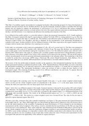
1.2 Theoretical Measurement Limits
The theoretical limit of sensitivity in any measurement is determined by the
noise generated by the resistances present in the circuit. As discussed in
Sections 2.6.5 and 3.2.2, voltage noise is proportional to the square root of
the resistance, bandwidth, and absolute temperature. Figure 1-2 shows theoretical
voltage measurement limits at room temperature (300K) with a
response time of 0.1 second to ten seconds. Note that high source resistance
limits the theoretical sensitivity of the voltage measurement. While it’s
certainly possible to measure a 1µV signal that has a 1Ω source resistance,
it’s not possible to measure that same 1µV signal level from a 1TΩ source.
Even with a much lower 1MΩ source resistance, a 1µV measurement is near
theoretical limits, so it would be very difficult to make using an ordinary
DMM.
In addition to having insufficient voltage or current sensitivity (most
DMMs are no more sensitive than 1µV or 1nA per digit), DMMs have high
Low Level DC Measuring Instruments 1-3

FIGURE 1-2: Theoretical Limits of Voltage Measurements
1kV
10 3
Noise
Voltage
1V
Within theoretical limits
10 0
1mV
1µV
1nV
1pV
Near theoretical limits
Prohibited
by noise
10 —3
10 —6
10 —9
10 —12
10 0 10 3 10 6 10 9 10 12
1Ω 1kΩ 1MΩ 1GΩ 1TΩ
Source Resistance
input offset current 1 when measuring voltage and lower input resistance
compared to more sensitive instruments intended for low level DC measurements.
These characteristics cause errors in the measurement; refer to
Sections 2 and 3 for further discussion of them.
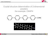
Given these DMM characteristics, it’s not possible to use a DMM to
measure signals at levels close to theoretical measurement limits, as shown
in Figure 1-3. However, if the source resistance is 1MΩ or less, or if the
desired resolution is no better than 0.1µV (with low source resistance), the
signal level isn’t “near theoretical limits,” and a DMM is adequate. If better
voltage sensitivity is desired, and the source resistance is low (as it must be
because of theoretical limitations), a nanovoltmeter provides a means of
measuring at levels much closer to the theoretical limits of measurement.
With very high source resistance values (for example, 1TΩ), a DMM isn’t a
suitable voltmeter. DMM input resistance ranges from 10MΩ to 10GΩ—several
orders of magnitude less than a 1TΩ source resistance, resulting in
severe input loading errors. Also, input currents are typically many
picoamps, creating large voltage offsets. However, because of its much higher
input resistance, an electrometer can make voltage measurements at levels
that approach theoretical limits. A similar situation exists for low level
current measurements; DMMs generally have a high input voltage drop
1
Input current flows in the input lead of an active device or instrument. With voltage measurements, the
input current is ideally zero; thus, any input current represents an error. With current measurements, the
signal current becomes the input current of the measuring instrument. However, some background current
is always present when no signal current is applied to the instrument input. This unwanted current
is the input offset current (often called just the offset current) of the instrument.
The source and test connections can also generate unwanted offset currents and offset voltages.
A leakage current is another unwanted error current resulting from voltage across an undesired resistance
path (called leakage resistance). This current, combined with the offset current, is the total error
current.
1-4 SECTION 1

FIGURE 1-3: Typical Digital Multimeter (DMM), Nanovoltmeter (nVM), Nanovolt
Preamplifier (nV PreAmp), and Electrometer Limits of Measurement at
Various Source Resistances
1V
10 0
Noise
Voltage
1mV
10 –3
Electrometer
DMM
nVM
nV PreAmp
1µV
1nV
10 –6
10 –9
1pV
10 –3
1mΩ
10 0 10 3 10 6 10 9 10 12
1Ω 1kΩ 1MΩ 1GΩ 1TΩ
Source Resistance
10 15
1PΩ
10 –12
(input burden), which affects low level current measurements, and DMM
resolution is generally no better than 1nA. Thus, an electrometer or picoammeter
with its much lower input burden and better sensitivity will operate
at levels much closer to the theoretical (and practical) limits of low current
measurements.
1.3 Instrument Definitions
A number of different types of instruments are available to make DC measurements,
including electrometers, DMMs, nanovoltmeters, picoammeters,
SMUs (source-measure units), SourceMeter instruments, low current preamps,
and micro-ohmmeters. The following paragraphs discuss and compare
the important characteristics of these instruments.
1.3.1 The Electrometer
An electrometer is a highly refined DC multimeter. As such, it can be used
for many measurements performed by a conventional DC multimeter.
Additionally, an electrometer’s special input characteristics and high sensitivity
allow it to make voltage, current, resistance, and charge measurements
far beyond the capabilities of a conventional DMM.
An electrometer must be used when any of the following conditions
exist:
1. The task requires an extended measurement range unavailable with
conventional instruments, such as for detecting or measuring:
• Currents less than 10nA (10 –8 A).
• Resistances greater than 1GΩ (10 9 Ω).
Low Level DC Measuring Instruments 1-5

2. Circuit loading must be minimized, such as when:
• Measuring voltage from a source resistance of 100MΩ or higher.
• Measuring current when input voltage drop (burden) of less than a
few hundred millivolts is required (when measuring currents from
sources of a few volts or less).
3. Charge measurement is required.
4. Measuring signals at or near Johnson noise limitations (as indicated in
Figure 1-2).
In addition to their versatility, electrometers are easy to operate, reliable,
and rugged.
Voltmeter Function
The input resistance of an electrometer voltmeter is extremely high, typically
greater than 100TΩ (10 14 Ω). Furthermore, the input offset current is
less than 3fA (3×10 –15 A). These characteristics describe a device that can
measure voltage with a very small amount of circuit loading.
Because of the high input resistance and low offset current, the electrometer
voltmeter has minimal effect on the circuit being measured. As a
result, the electrometer can be used to measure voltage in situations where
an ordinary multimeter would be unusable. For example, the electrometer
can measure the voltage on a 500pF capacitor without significantly discharging
the device; it can also measure the potential of piezoelectric crystals
and high impedance pH electrodes.
Ammeter Function
As an ammeter, the electrometer is capable of measuring extremely low currents,
limited only by theoretical limits or by the instrument’s input offset
current. It also has a much lower voltage burden than conventional DMMs.
With its extremely low input offset current and minimal input voltage
burden, it can detect currents as low as 1fA (10 –15 A). Because of this high
sensitivity, it’s suitable for measuring the current output of photomultipliers
and ion chambers, as well as very low currents in semiconductors, mass
spectrometers, and other devices.
Ohmmeter Function
An electrometer may measure resistance by using either a constant-current
or a constant-voltage method. If using the constant-current method, the
electrometer’s high input resistance and low offset current enables measurements
up to 200GΩ. When using the constant-voltage method, the electrometer
applies a constant voltage to the unknown resistance, measures
the current, and then calculates the resistance. This is the preferred method
because it allows the unknown resistor to be tested at a known voltage. An
electrometer can measure resistances up to 10PΩ (10 16 Ω) using this
method.
1-6 SECTION 1

Coulombmeter Function
Current integration and measurement of charge are electrometer coulombmeter
capabilities not found in multimeters. The electrometer coulombmeter
can detect charge as low as 10fC (10 –14 C). It’s equivalent to an active
integrator and, therefore, has low voltage burden, typically less than 100µV.
The coulombmeter function can measure lower currents than the
ammeter function can, because no noise is contributed by internal resistors.
Currents as low as 1fA (10 –15 A) may be detected using this function. See
Section 2.3.8 for further details.
1.3.2 The DMM
Digital multimeters vary widely in performance, from low cost handheld 3 1 ⁄2-
digit units to high precision system DMMs. While there are many models
available from a wide variety of manufacturers, none approaches the theoretical
limits of measurement discussed previously. These limitations don’t
imply that DMMs are inadequate instruments; they simply point out the fact
that the vast majority of measurements are made at levels far from theoretical
limits, and DMMs are designed to meet these more conventional measurement
needs.
Although low level measurements are by definition those that are close
to theoretical limits, and are thus outside the range of DMMs, advances in
technology are narrowing the gap between DMMs and dedicated low level
instruments. For example, the most sensitive DMMs can detect DC voltages
as low as 10nV, resolve DC currents down to 10pA, and measure resistances
as high as 1GΩ. While these characteristics still fall far short of the corresponding
capabilities of more sensitive instruments like the electrometer
described previously, all the measurement theory and accuracy considerations
in this book apply to DMM measurements as well as to nanovoltmeter,
picoammeter, electrometer, or SMU measurements. The difference is only a
matter of degree; when making measurements close to theoretical limits, all
measurement considerations are vitally important. When measuring at levels
far from theoretical limits, only a few basic considerations (accuracy,
loading, etc.) are generally of concern.
1.3.3 The Nanovoltmeter
A nanovoltmeter is a very sensitive voltage meter. As shown in Figure 1-3,
this type of instrument is optimized to provide voltage measurements near
the theoretical limits from low source resistances, in contrast to the electrometer,
which is optimized for use with high source resistances.
Compared to an electrometer, the voltage noise and drift are much lower,
and the current noise and drift are much higher. Input resistance is usually
similar to that of a DMM and is much lower than that of an electrometer.
As is the case with electrometers, nanovoltmeters are just as reliable and
easy to operate as DMMs. Their distinguishing characteristic is their voltage
sensitivity, which can be as good as 1pV. Most nanovoltmeters aren’t multi-
Low Level DC Measuring Instruments 1-7

function instruments and are correspondingly less complex than
electrometers.
1.3.4 The Picoammeter
A picoammeter is an ammeter built along the lines of the ammeter function
of an electrometer. When compared with an electrometer, a picoammeter
has a similar low voltage burden, similar or faster speed, less sensitivity, and
a lower price. It may also have special characteristics, such as high speed
logarithmic response or a built-in voltage source.
1.3.5 The Source-Measure Unit
As its name implies, a source-measure unit (SMU) has both measuring and
sourcing capabilities. Adding current and voltage sourcing capabilities to a
measuring instrument provides an extra degree of versatility for many low
level measurement applications. For example, very high resistance values
can be determined by applying a voltage across a device and measuring the
resulting current. The added sourcing functions also make a SMU more convenient
and versatile than using separate instruments for such applications
as generating I-V curves of semiconductors and other types of devices.
The typical SMU provides the following four functions:
• Measure voltage
• Measure current
• Source voltage
• Source current
These functions can be used separately or they can be used together in
the following combinations:
• Simultaneously source voltage and measure current, or
• Simultaneously source current and measure voltage.
SMUs have a number of electrometer-like characteristics that make
them suitable for low level measurements. The input resistance is very high
(typically 100TΩ or more), minimizing circuit loading when making voltage
measurements from high impedance sources. The current measurement
sensitivity is also similar to that of the electrometer picoammeter—typically
as low as 10fA.
Another important advantage of many source-measure units is their
sweep capability. Either voltage or current can be swept across the desired
range at specified increments, and the resulting current or voltage can be
measured at each step. Built-in source-delay-measure cycles allow optimizing
measurement speed while ensuring sufficient circuit settling time to
maintain measurement integrity.
1-8 SECTION 1

1.3.6 The SourceMeter ® Instrument
The SourceMeter instrument is very similar to the source-measure unit in
many ways, including its ability to source and measure both current and
voltage and to perform sweeps. In addition, a SourceMeter instrument can
display the measurements directly in resistance, as well as voltage and
current.
The typical SourceMeter instrument doesn’t have as high an input
impedance or as low a current capability as a source-measure unit. The
SourceMeter instrument is designed for general-purpose, high speed production
test applications. It can be used as a source for moderate to low
level measurements and for research applications.
Unlike a DMM, which can make a measurement at only one point, a
SourceMeter instrument can be used to generate a family of curves, because
it has a built-in source. This is especially useful when studying semiconductor
devices and making materials measurements.
When used as a current source, a SourceMeter instrument can be used
in conjunction with a nanovoltmeter to measure very low resistances by
automatically reversing the polarity of the source to correct for offsets.
1.3.7 The Low Current Preamp
Some SMUs and SourceMeter instruments may have a remote low current
preamp. With this design, the sensitive amplifier circuitry is separate from
the SMU or SourceMeter instrument. This makes it possible to place the
most sensitive part of the instrument very close to the device being tested,
thereby eliminating a major source of error, the noise and leakage from the
cables themselves.
1.3.8 The Micro-ohmmeter
A micro-ohmmeter is a special type of ohmmeter designed especially for
making low level resistance measurements. While the techniques used for
making resistance measurements are similar to those used in a DMM, microohmmeter
circuits are optimized for making low level measurements. The
typical micro-ohmmeter can resolve resistances as low as 10µΩ.
Measurements made using the micro-ohmmeter are always performed
using the four-wire technique in order to minimize errors caused by test
leads and connections. The typical micro-ohmmeter also has additional features
such as offset compensation and dry circuit testing to optimize low
resistance measurements. Offset compensation is performed by pulsing the
test current to cancel offsets from thermoelectric EMFs. The dry circuit test
mode limits the voltage across the unknown resistance to a very small value
(typically

1.4 Understanding Instrument Specifications
Knowing how to interpret instrument specifications properly is an important
aspect of making good low level measurements. Although instrument
accuracy is probably the most important of these specifications, there are
several other factors to consider when reviewing specifications, including
noise, deratings, and speed.
1.4.1 Definition of Accuracy Terms
This section defines a number of terms related to instrument accuracy.
Some of these terms are further discussed in subsequent paragraphs. Table
1-1 summarizes conversion factors for various specifications associated with
instruments.
SENSITIVITY - the smallest change in the signal that can be detected.
RESOLUTION - the smallest portion of the signal that can be observed.
REPEATABILITY - the closeness of agreement between successive measurements
carried out under the same conditions.
REPRODUCIBILITY - the closeness of agreement between measurements of
the same quantity carried out with a stated change in conditions.
ABSOLUTE ACCURACY - the closeness of agreement between the result of a
measurement and its true value or accepted standard value. Accuracy
is often separated into gain and offset terms.
RELATIVE ACCURACY - the extent to which a measurement accurately
reflects the relationship between an unknown and a reference value.
ERROR - the deviation (difference or ratio) of a measurement from its true
value. Note that true values are by their nature indeterminate.
RANDOM ERROR - the mean of a large number of measurements influenced
by random error matches the true value.
SYSTEMATIC ERROR - the mean of a large number of measurements influenced
by systematic error deviates from the true value.
UNCERTAINTY - an estimate of the possible error in a measurement, i.e., the
estimated possible deviation from its actual value. This is the opposite
of accuracy.
“Precision” is a more qualitative term than many of those defined here.
It refers to the freedom from uncertainty in the measurement. It’s often
applied in the context of repeatability or reproducibility, but it shouldn’t be
used in place of “accuracy.”
1.4.2 Accuracy
One of the most important considerations in any measurement situation is
reading accuracy. For any given test setup, a number of factors can affect
accuracy. The most important factor is the accuracy of the instrument itself,
which may be specified in several ways, including a percentage of full scale,
1-10 SECTION 1

TABLE 1-1: Specification Conversion Factors
Number of time
Percent PPM Digits Bits dB
Portion
of 10V
constants to settle
to rated accuracy
10% 100000 1 3.3 –20 1 V 2.3
1% 10000 2 6.6 –40 100mV 4.6
0.1% 1000 3 10 –60 10mV 6.9
0.01% 100 4 13.3 –80 1mV 9.2
0.001% 10 5 16.6 –100 100 µV 11.5
0.0001% 1 6 19.9 –120 10 µV 13.8
0.00001% 0.1 7 23.3 –140 1µV 16.1
0.000001% 0.01 8 26.6 –160 100 nV 18.4
0.000001% 0.001 9 29.9 –180 10 nV 20.7
a percentage of reading, or a combination of both. Instrument accuracy
aspects are covered in the following paragraphs.
Other factors such as input loading, leakage resistance and current,
shielding, and guarding may also have a serious impact on overall accuracy.
These important measurement considerations are discussed in detail in
Sections 2 and 3.
Measurement Instrument Specifications
Instrument accuracy is usually specified as a percent of reading, plus a percentage
of range (or a number of counts of the least significant digit). For
example, a typical DMM accuracy specification may be stated as: ±(0.005%
of reading + 0.002% of range). Note that the percent of reading is most significant
when the reading is close to full scale, while the percent of range is
most significant when the reading is a small fraction of full scale.
Accuracy may also be specified in ppm (parts per million). Typically, this
accuracy specification is given as ±(ppm of reading + ppm of range). For
example, the DCV accuracy of a higher resolution DMM might be specified
as ±(25ppm of reading + 5ppm of range).
Resolution
The resolution of a digital instrument is determined by the number of
counts that can be displayed, which depends on the number of digits. A typical
digital electrometer might have 5 1 ⁄2 digits, meaning five whole digits
(each with possible values between 0 and 9) plus a leading half digit that
can take on the values 0 or ±1. Thus, a 5 1 ⁄2-digit display can show 0 to
199,999, a total of 200,000 counts. The resolution of the display is the ratio
of the smallest count to the maximum count (1/200,000 or 0.0005% for a
5 1 ⁄2-digit display).
Low Level DC Measuring Instruments 1-11

For example, the specification of ±(0.05% + 1 count) on a 4 1 ⁄2-digit
meter reading 10.000 volts corresponds to a total error of ±(5mV + 1mV)
out of 10V, or ±(0.05% of reading + 0.01% of reading), totaling ±0.06%.
Generally, the higher the resolution, the better the accuracy.
Sensitivity
The sensitivity of a measurement is the smallest change of the measured signal
that can be detected. For example, voltage sensitivity may be 1µV, which
simply means that any change in input signal less than 1µV won’t show up
in the reading. Similarly, a current sensitivity of 10fA implies that only
changes in current greater than that value will be detected.
The ultimate sensitivity of a measuring instrument depends on both its
resolution and the lowest measurement range. For example, the sensitivity
of a 5 1 ⁄2-digit DMM with a 200mV measurement range is 1µV.
Absolute and Relative Accuracy
As shown in Figure 1-4, absolute accuracy is the measure of instrument
accuracy that is directly traceable to the primary standard at the National
Institute of Standards and Technology (NIST). Absolute accuracy may be
specified as ±(% of reading + counts), or it can be stated as ±(ppm of reading
+ ppm of range), where ppm signifies parts per million of error.
FIGURE 1-4: Comparison of Absolute and Relative Accuracy
NIST
Standard
Secondary
Standard
Absolute
Accuracy
Measuring
Instrument
Relative
Accuracy
Device
Under Test
Relative accuracy (see Figure 1-4) specifies instrument accuracy to
some secondary reference standard. As with absolute accuracy, relative accuracy
can be specified as ±(% of reading + counts) or it may be stated as
±(ppm of reading + ppm of range).
1-12 SECTION 1

Transfer Stability
A special case of relative accuracy is the transfer stability, which defines
instrument accuracy relative to a secondary reference standard over a very
short time span and narrow ambient temperature range (typically within
five minutes and ±1°C). The transfer stability specification is useful in situations
where highly accurate measurements must be made in reference to a
known secondary standard.
Calculating Error Terms from Accuracy Specifications
To illustrate how to calculate measurement errors from instrument specifications,
assume the following measurement parameters:
Accuracy: ±(25ppm of reading + 5ppm of range)
Range: 2V
Input signal: 1.5V
The error is calculated as:
Error = 1.5(25 × 10 –6 ) + 2(5 × 10 –6 )
= (37.5 × 10 –6 ) + (10 × 10 –6 )
= 47.5 × 10 –6
Thus, the reading could fall anywhere within the range of 1.5V ±
47.5µV, an error of ±0.003%.
1.4.3 Deratings
Accuracy specifications are subject to deratings for temperature and time
drift, as discussed in the following paragraphs.
Temperature Coefficient
The temperature of the operating environment can affect accuracy. For this
reason, instrument specifications are usually given over a defined temperature
range. Keithley accuracy specifications on newer electrometers, nanovoltmeters,
DMMs, and SMUs are usually given over the range of 18°C to
28°C. For temperatures outside of this range, a temperature coefficient such
as ±(0.005 % + 0.1 count)/°C or ±(5ppm of reading + 1ppm of range)/°C
is specified. As with the accuracy specification, this value is given as a percentage
of reading plus a number of counts of the least significant digit (or
as a ppm of reading plus ppm of range) for digital instruments. If the instrument
is operated outside the 18°C to 28°C temperature range, this figure
must be taken into account, and errors can be calculated in the manner
described previously for every degree less than 18°C or greater than 28°C.
Time Drift
Most electronic instruments, including electrometers, picoammeters, nanovoltmeters,
DMMs, SMUs, and SourceMeter instruments, are subject to
changes in accuracy and other parameters over a long period of time,
whether or not the equipment is operating. Because of these changes,
instrument specifications usually include a time period beyond which the
Low Level DC Measuring Instruments 1-13

instrument’s accuracy cannot be guaranteed. The time period is stated in
the specifications, and is typically over specific increments such as 90 days
or one year. As noted previously, transfer stability specifications are defined
for a much shorter period of time—typically five or 10 minutes.
1.4.4 Noise and Noise Rejection
Noise is often a consideration when making virtually any type of electronic
measurement, but noise problems can be particularly severe when making
low level measurements. Thus, it’s important that noise specifications and
terms are well understood when evaluating the performance of an instrument.
Normal Mode Rejection Ratio
Normal mode rejection ratio (NMRR) defines how well the instrument
rejects or attenuates noise that appears between the HI and LO input terminals.
Noise rejection is accomplished by using the integrating A/D converter
to attenuate noise at specific frequencies (usually 50 and 60Hz) while
passing low frequency or DC normal mode signals. As shown in Figure
1-5, normal mode noise is an error signal that adds to the desired input
signal. Normal mode noise is detected as a peak noise or deviation in a DC
signal. The ratio is calculated as:
peak normal mode noise
NMRR = 20 log _______________________________
FIGURE 1-5: Normal Mode Noise
[ peak measurement deviation ]
Measuring
Instrument
HI
LO
Noise
Signal
Normal mode noise can seriously affect measurements unless steps are
taken to minimize the amount added to the desired signal. Careful shielding
will usually attenuate normal mode noise, and many instruments have
internal filtering to reduce the effects of such noise even further.
Common Mode Rejection Ratio
Common mode rejection ratio (CMRR) specifies how well an instrument
rejects noise signals that appear between both input high and input low and
chassis ground, as shown in Figure 1-6. CMRR is usually measured with a
1kΩ resistor imbalance in one of the input leads.
1-14 SECTION 1

FIGURE 1-6: Common Mode Noise
Measuring
Instrument
HI
LO
R imbalance
Signal
(usually 1kΩ)
Noise
Although the effects of common mode noise are usually less severe than
normal mode noise, this type of noise can still be a factor in sensitive measurement
situations. To minimize common mode noise, connect shields
only to a single point in the test system.
Noise Specifications
Both NMRR and CMRR are generally specified in dB at 50 and 60Hz, which
are the interference frequencies of greatest interest. (CMRR is often specified
at DC as well.) Typical values for NMRR and CMRR are >80dB and
>120dB respectively.
Each 20dB increase in noise rejection ratio reduces noise voltage or current
by a factor of 10. For example, a rejection ratio of 80dB indicates noise
reduction by a factor of 10 4 , while a ratio of 120dB shows that the common
mode noise would be reduced by a factor of 10 6 . Thus, a 1V noise signal
would be reduced to 100µV with an 80dB rejection ratio and down to 1µV
with a 120dB rejection ratio.
1.4.5 Speed
Instrument measurement speed is often important in many test situations.
When specified, measurement speed is usually stated as a specific number
of readings per second for given instrument operating conditions. Certain
factors such as integration period and the amount of filtering may affect
overall instrument measurement speed. However, changing these operating
modes may also alter resolution and accuracy, so there is often a tradeoff
between measurement speed and accuracy.
Instrument speed is most often a consideration when making low
impedance measurements. At higher impedance levels, circuit settling times
become more important and are usually the overriding factor in determining
overall measurement speed. Section 2.6.4 discusses circuit settling time
considerations in more detail.
Low Level DC Measuring Instruments 1-15

1.5 Circuit Design Basics
Circuits used in the design of many low level measuring instruments,
whether a voltmeter, ammeter, ohmmeter, or coulombmeter, generally use
circuits that can be understood as operational amplifiers. Figure 1-7 shows
a basic operational amplifier. The output voltage is given by:
V O = A (V 1 – V 2 )
FIGURE 1-7: Basic Operational Amplifier
V 1
+
–
V 2
A
V O
COMMON
V O = A (V 1 –V 2 )
The gain (A) of the amplifier is very large, a minimum of 10 4 to 10 5 , and
often 10 6 . The amplifier has a power supply (not shown) referenced to the
common lead.
Current into the op amp inputs is ideally zero. The effect of feedback
properly applied is to reduce the input voltage difference (V 1 – V 2 ) to zero.
1.5.1 Voltmeter Circuits
Electrometer Voltmeter
The operational amplifier becomes a voltage amplifier when connected as
shown in Figure 1-8. The offset current is low, so the current flowing
through R A and R B is the same. Assuming the gain (A) is very high, the voltage
gain of the circuit is defined as:
V O = V 2 (1 + R A /R B )
Thus, the output voltage (V O ) is determined both by the input voltage
(V 2 ), and amplifier gain set by resistors R A and R B . Given that V 2 is applied
to the amplifier input lead, the high input resistance of the operational
amplifier is the only load on V 2 , and the only current drawn from the source
is the very low input offset current of the operational amplifier. In many
electrometer voltmeters, R A is shorted and R B is open, resulting in
unity gain.
1-16 SECTION 1

FIGURE 1-8: Voltage Amplifier
+
–
V 2
A
R A
V O
V 1
R B
V O = V 2 (1 + R A /R B )
Nanovoltmeter Preamplifier
The same basic circuit configuration shown in Figure 1-8 can be used as an
input preamplifier for a nanovoltmeter. Much higher voltage gain is
required, so the values of R A and R B are set accordingly; a typical voltage
gain for a nanovoltmeter preamplifier is 10 3 .
Electrometer and nanovoltmeter characteristics differ, so the operational
amplifier requirements for these two types of instruments are also
somewhat different. While the most important characteristics of the electrometer
voltmeter operational amplifier are low input offset current and
high input impedance, the most important requirement for the nanovoltmeter
input preamplifier is low input noise voltage.
1.5.2 Ammeter Circuits
There are two basic techniques for making current measurements: these are
the shunt ammeter and the feedback ammeter techniques. DMMs and older
electrometers use the shunt method, while picoammeters and the AMPS
function of electrometers use the feedback ammeter configuration only.
Shunt Ammeter
Shunting the input of a voltmeter with a resistor forms a shunt ammeter, as
shown in Figure 1-9. The input current (I IN ) flows through the shunt resistor
(R S ). The output voltage is defined as:
V O = I IN R S (1 + R A /R B )
For several reasons, it’s generally advantageous to use the smallest possible
value for R S .
First, low value resistors have better accuracy, time and temperature stability,
and voltage coefficient than high value resistors. Second, lower resistor
Low Level DC Measuring Instruments 1-17

values reduce the input time constant and result in faster instrument
response time. To minimize circuit loading, the input resistance (R S ) of an
ammeter should be small, thus reducing the voltage burden (V 2 ). However,
note that reducing the shunt resistance will degrade the signal-to-noise ratio.
FIGURE 1-9: Shunt Ammeter
R S
I IN
V O = I IN R S (1 + R A /R B )
V 2
+
—
A
R A
V O
V 1
R B
Feedback Ammeter
In this configuration, shown in Figure 1-10, the input current (I IN ) flows
through the feedback resistor (R F ). The low offset current of the amplifier
(A) changes the current (I IN ) by a negligible amount. The amplifier output
voltage is calculated as:
V O = –I IN R F
Thus, the output voltage is a measure of input current, and overall sensitivity
is determined by the feedback resistor (R F ). The low voltage burden
(V 1 ) and corresponding fast rise time are achieved by the high gain op amp,
which forces V 1 to be nearly zero.
FIGURE 1-10: Feedback Ammeter
R F
I IN
Input
+
V 1
–
A
V O
Output
V O = –I IN R F
1-18 SECTION 1

Picoammeter amplifier gain can be changed as in the voltmeter circuit
by using the combination shown in Figure 1-11. Here, the addition of R A
and R B forms a “multiplier,” and the output voltage is defined as:
V O = –I IN R F (1 + R A /R B )
FIGURE 1-11: Feedback Ammeter with Selectable Voltage Gain
I IN
R F
V O = –I IN R F (1 + R A /R B )
+
V 1
–
A
R A
V O
R B
High Speed Picoammeter
The rise time of a feedback picoammeter is normally limited by the time
constant of the feedback resistor (R F ) and any shunting capacitance (C F ). A
basic approach to high speed measurements is to minimize stray shunting
capacitance through careful mechanical design of the picoammeter.
Remaining shunt capacitance can be effectively neutralized by a slight
modification of the feedback loop, as shown in Figure 1-12. If the time constant
R 1 C 1 is made equal to the time constant R F C F , the shaded area of the
circuit behaves exactly as a resistance R F with zero C F . The matching of time
constants in this case is fairly straightforward, because the capacitances
involved are all constant and aren’t affected by input capacitances.
Logarithmic Picoammeter
A logarithmic picoammeter can be formed by replacing the feedback resistor
in a picoammeter with a diode or transistor exhibiting a logarithmic voltage-current
relationship, as shown in Figure 1-13. The output voltage (and
the meter display) is then equal to the logarithm of the input current. As a
result, several decades of current can be read on the meter without changing
the feedback element.
Low Level DC Measuring Instruments 1-19

FIGURE 1-12: Neutralizing Shunt Capacitance
C F
R 1
C 1
–
A
I IN +
FIGURE 1-13: Logarithmic Picoammeter
–
A
I IN +
R F
V O
V O
The main advantage of a logarithmic picoammeter is its ability to follow
current changes over several decades without range changing.
The big disadvantage is the loss of accuracy and resolution, but some
digital picoammeters combine accuracy and dynamic range by combining
autoranging and digital log conversion.
If two diodes are connected in parallel, back-to-back, this circuit will
function with input signals of either polarity.
1-20 SECTION 1

Using a small-signal transistor in place of a diode produces somewhat
better performance. Figure 1-14 shows an NPN transistor and a PNP transistor
in the feedback path to provide dual polarity operation.
FIGURE 1-14: Dual Polarity Log Current to Voltage Converter
1000pF
Input
–
+
A
Output
Remote Preamp Circuit (Source V, Measure I Mode)
Figure 1-15 illustrates a typical preamp circuit. In the Source V, Measure I
mode, the SMU applies a programmed voltage and measures the current
flowing from the voltage source. The sensitive input is surrounded by a
guard, which can be carried right up to the DUT for fully guarded measurements.
The remote preamp amplifies the low current signal passing through
the DUT; therefore, the cable connecting the remote preamp to the measurement
mainframe carries only high level signals, minimizing the impact of
cable noise.
FIGURE 1-15: Remote Preamp in Source V, Measure I Mode
To
measurement
mainframe of
SMU or
SourceMeter
AI IN
Guard
LO
A
I IN
Input/
Output
HI
To DUT
Low Level DC Measuring Instruments 1-21

1.5.3 Coulombmeter Circuit
The coulombmeter measures electrical charge that has been stored in a
capacitor or that might be produced by some charge generating process.
For a charged capacitor, Q = CV, where Q is the charge in coulombs on
the capacitor, C is the capacitance in farads, and V is the potential across the
capacitor in volts. Using this relationship, the basic charge measuring
scheme is to transfer the charge to be measured to a capacitor of known
value and then measure the voltage across the known capacitor; thus,
Q = CV.
The electrometer is ideal for charge measurements, because the low offset
current won’t alter the transferred charge during short time intervals
and the high input resistance won’t allow the charge to bleed away.
Electrometers use a feedback circuit to measure charge, as shown in
Figure 1-16. The input capacitance of this configuration is AC F . Thus, large
effective values of input capacitance are obtained using reasonably sized
capacitors for C F .
FIGURE 1-16: Feedback Coulombmeter
C F
–
+
A
V O
1.5.4 High Resistance Ohmmeter Circuits
Electrometer Picoammeter and Voltage Source
In this configuration (Figure 1-17), a voltage source (V S ) is placed in series
with an unknown resistor (R X ) and an electrometer picoammeter. The voltage
drop across the picoammeter is small, so essentially all the voltage
appears across R X , and the unknown resistance can be computed from the
sourced voltage and the measured current (I).
The advantages of this method are that it’s fast and, depending on the
power supply voltage and insulating materials, it allows measuring extremely
high resistance. Also, with an adjustable voltage source, the voltage
dependence of the resistance under test can be obtained directly.
1-22 SECTION 1

FIGURE 1-17: High Resistance Measurement Using External Voltage Source
R X
R X = V S
I
V S
LO
Electrometer
Picoammeter
Electrometer Ohmmeter Using Built-In Current Source
FIGURE 1-18: Electrometer Ohmmeter with Built-In Current Source
Built-In Current Source
V S
I = V S /R
V 1 = I R X
Usually, this method requires two instruments: a voltage source and a
picoammeter or electrometer. Some electrometers and picoammeters, however,
have a built-in voltage source and are capable of measuring the resistance
directly.
Figure 1-18 shows the basic configuration of an alternative form of electrometer
ohmmeter. A built-in constant-current source, formed by V S and R,
forces a known current through the unknown resistance (R X ). The resulting
voltage drop is proportional to the unknown resistance and is indicated by
the meter as resistance, rather than voltage.
R
I
I
HI
–
+
A
R X C S V 1
V O
Low Level DC Measuring Instruments 1-23

The disadvantage of this method is that the voltage across the unknown
is a function of its resistance, so it cannot be easily controlled. Very high
resistances tend to have large voltage coefficients; therefore, measurements
made with a constant voltage are more meaningful. In addition, the
response speed for resistances greater than 10GΩ will be rather slow. This
limitation can be partially overcome by guarding.
Electrometer Ohmmeter with Guarded Ohms Mode
Figure 1-19 shows a modification of the circuit in Figure 1-18 in which the
HI input node is surrounded with a guard voltage from the operational
amplifier output. The amplifier has unity gain, so this guard voltage is virtually
the same potential as V 1 and the capacitance (C S ) of the input cable is
largely neutralized, resulting in much faster measurements of resistances
greater than 10GΩ.
FIGURE 1-19: Electrometer Ohmmeter with Guarded Ohms
Built-In Current Source
V S
I = V S /R
V 1 = I R X
R
I
–
A
+
R X C S Guard
V 1
V O
The guarded mode also significantly reduces the effect of input cable
leakage resistance, as discussed in Section 2.4.2.
Electrometer Voltmeter and External Current Source
In this method, shown in Figure 1-20, a current source generates current
(I), which flows through the unknown resistor (R X ). The resulting voltage
drop is measured with an electrometer voltmeter, and the value of R X is calculated
from the voltage and current.
1-24 SECTION 1

FIGURE 1-20: High Resistance Measurement Using External Current Source with
Electrometer Voltmeter
External
Current
Source
I R X V 1
HI
LO
Electrometer
Voltmeter
V 1 = I R X
If the current source has a buffered ×1 output, a low impedance voltmeter,
such as a DMM, may be used to read the voltage across R X . This
arrangement is shown in Figure 1-21.
FIGURE 1-21: High Resistance Measurement Using a True Current Source with
a DMM
—
A
+
HI
×1 Output
I R X V 1
V O
LO
DMM
Constant-Current Source
with Buffered ×1 Output
V O
≈ V 1 = I R X
1.5.5 Low Resistance Ohmmeter Circuits
Nanovoltmeter and External Current Source
If the electrometer in Figure 1-20 is replaced with a nanovoltmeter, the circuit
can be used to measure very low resistances (

DMM Ohmmeter
The typical DMM uses the ratiometric technique shown in Figure 1-22 to
make resistance measurements. When the resistance function is selected, a
series circuit is formed between the ohms voltage source, a reference resistance
(R REF ), and the resistance being measured (R X ). The voltage causes a
current to flow through the two resistors. This current is common to both
resistances, so the value of the unknown resistance can be determined by
measuring the voltage across the reference resistance and across the
unknown resistance and calculating as:
SENSE HI – SENSE LO
R X = R REF · __________________________
REF HI – REF LO
FIGURE 1-22: Ratiometric Resistance Measurement
Ref HI
R REF
R S
V REF
R 1
Input HI
Ref LO
R X
R 2
Four-wire
connection
only
R 3
Sense HI
Sense LO
V SENSE
Sense HI
Sense LO
R S
R 4
Input LO
R X = R REF
V SENSE
V REF
R 1 , R 2 , R 3 , R 4 = lead resistance
The resistors (R S ) provide automatic two-wire or four-wire resistance
measurements. When used in the two-wire mode, the measurement will
include the lead resistance, represented by R 1 and R 4 . When the unknown
resistance is low, perhaps less than 100Ω, the four-wire mode will give much
better accuracy. The sense lead resistance, R 2 and R 3 , won’t cause significant
error because the sense circuit has very high impedance.
1-26 SECTION 1

Micro-ohmmeter
The micro-ohmmeter also uses the four-wire ratiometric technique, which
is shown in Figure 1-23. It doesn’t have the internal resistors (R S ), as in the
DMM, so all four leads must be connected to make a measurement. Also,
the terminals that supply test current to the unknown resistance are labeled
Source HI and Source LO.
FIGURE 1-23: Micro-ohmmeter Resistance Measurement
Ref HI
R REF
V REF
R 1
Source HI
Ref LO
R X
R 2
Sense HI
V SENSE
Sense HI
R 3
Sense LO
Sense LO
R 4
Source LO
R X = R REF · VSENSE
V REF
The pulsed drive mode, shown in Figure 1-24, allows the microohmmeter
to cancel stray offset voltages in the unknown resistance being
measured. During the measurement cycle, the voltage across the unknown
resistance is measured twice, once with the drive voltage on, and a second
time with the drive voltage turned off. Any voltage present when the drive
voltage is off represents an offset voltage and will be subtracted from the
voltage measured when the drive voltage is on, providing a more accurate
measurement of the resistance.
The dry circuit test mode, shown in Figure 1-25, adds a resistor across
the source terminals to limit the open-circuit voltage to less than 20mV. This
prevents breakdown of any insulating film in the device being tested and
gives a better indication of device performance with low level signals. The
meter must now measure the voltage across this resistor (R SH ), as well as the
voltage across the reference resistor and the unknown resistor. See Section
3.3.5 for more information on dry circuit testing.
Low Level DC Measuring Instruments 1-27

FIGURE 1-24:
Micro-ohmmeter in Pulse Mode
Ref HI
R REF V REF
R 1 Source HI
Ref LO S 1
R 2 Sense HI
Sense HI
R X V X V SENSE
V OS
R 3 Sense LO
Sense LO
R 4
Source LO
R X = R REF · VSENSE 1 – V SENSE 2
V REF
where V SENSE 1 is measured with S 1 closed, and is equal to V X + V OS , and
V SENSE 2 is measured with S 1 open, and is equal to V OS .
FIGURE 1-25:
Micro-ohmmeter with Dry Circuit On
Ref HI
R REF
V REF
R 1
Source HI
Ref LO
Sense HI
R 2
Sense HI
Shunt HI
R X
V SENSE
R SH
V SH
R 3
Sense LO
Shunt LO
Sense LO
R 4
Source LO
R X =
V SENSE
V REF V SH
R REF
R SH
1-28 SECTION 1

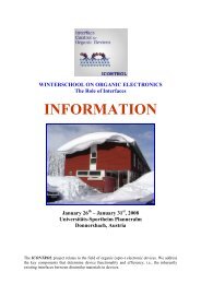
FIGURE 1-26: Typical Digital Electrometer
Amps
Coulombs
Function/Range
Digital Multimeters (DMMs)
Most DMMs include five measurement functions: DC volts, AC volts, ohms,
DC amps, and AC amps. As shown in Figure 1-27, various signal processing
circuits are used to convert the input signal into a DC voltage that can be
converted to digital information by the A/D converter.
The DC and AC attenuator circuits provide ranging for the AC and DC
functions. The AC converter changes AC signals to DC, while the ohms con-
Microprocessor
Display
IEEE-488
Interface
Volts
Ohms
A/D
Converter
Input
HI
LO
Zero
Check
–
A
+
Ranging
Amplifier
2V Analog
Output
Preamp
Output
Volts, Ohms
Guard
Output
Amps, Coulombs
1.5.6 Complete Instruments
Digital Electrometers
Figure 1-26 is a block diagram of a typical digital electrometer. The analog
section is similar to the circuitry discussed previously. An electrometer preamplifier
is used at the input to increase sensitivity and raise input resistance.
The output of the main amplifier is applied to both the analog output
and the A/D converter. Range switching and function switching, instead of
being performed directly, are controlled by the microprocessor.
The microprocessor also controls the A/D converter and supervises all
other operating aspects of the instrument. The input signal to the A/D converter
is generally 0–2V DC. After conversion, the digital data is sent to the
display and to the digital output port (IEEE- 488 or RS-232).
Low Level DC Measuring Instruments 1-29

FIGURE 1-27: DMM Block Diagram
AC
Attenuator
AC
Converter
Digital
Display
HI
INPUT
Amps
AC
DC
Ohms
DC
Attenuator
Ohms
Converter
AC
DC
Ohms
A/D
Converter
Precision
Reference
Digital
Output
Ports
(IEEE-488,
RS-232,
Ethernet)
Precision
Shunts
LO
verter provides a DC analog signal for resistance measurements. Precision
shunts are used to convert currents to voltages for the amps functions.
Once the input signal is appropriately processed, it’s converted to digital
information by the A/D converter. Digital data is then sent to the display
and to the digital output port (IEEE-488, RS-232, or Ethernet).
Nanovoltmeters
A nanovoltmeter is a sensitive voltmeter optimized to measure very low voltages.
As shown in Figure 1-28, the nanovoltmeter incorporates a low noise
preamplifier, which amplifies the signal to a level suitable for A/D conversion
(typically 2–3V full scale). Specially designed preamplifier circuits
ensure that unwanted noise, thermoelectric EMFs, and offsets are kept to an
absolute minimum.
FIGURE 1-28: Typical Nanovoltmeter
HI
DCV Input
LO
Low-Noise
Preamplifier
Range
Switching
A/D
Converter
Display
IEEE-488,
RS-232
Offset
Compensation
Microprocessor
1-30 SECTION 1

In order to cancel internal offsets, an offset or drift compensation circuit
allows the preamplifier offset voltage to be measured during specific
phases of the measurement cycle. The resulting offset voltage is subsequently
subtracted from the measured signal to maximize measurement
accuracy.
Once the preamplifier amplifies the signal, it’s converted to digital
information by the A/D converter. Digital data is then sent to the display and
the IEEE-488 interface.
SMUs
The SMU provides four functions in one instrument: measure voltage, measure
current, source voltage and source current. Generally, such instruments
can simultaneously source voltage and measure current or simultaneously
source current and measure voltage.
When configured to Source I and Measure V (as shown in Figure 1-29),
the SMU will function as a high impedance current source with voltage
measure (and voltage limit) capability.
Selecting either local or remote sense determines where the voltage
measurement will be made. In local sense, the voltage is measured at the
output of the SMU. In remote sense, the voltage is measured at the device
under test, eliminating any voltage drops due to lead resistance.
The driven guard (×1 Buffer) ensures that the Guard and Output HI terminals
are always at the same potential. Proper use of Guard virtually eliminates
leakage paths in the cable, test fixture, and connectors. When configured
to Source V and Measure I (as shown in Figure 1-30), the SMU will
function as a low impedance voltage source with current measure (and current
limit) capability.
SourceMeter Instrument
Like an SMU, a SourceMeter instrument can source current, source voltage,
measure current and measure voltage. However, the SourceMeter instrument
also has a sixth terminal, guard sense, which allows making more
accurate measurements of networks. When configured to source current as
shown in Figure 1-31, the SourceMeter unit functions as a high impedance
current source with voltage limit capability and it can measure current, voltage,
or resistance.
For voltage measurements, the sense selection (two-wire local or fourwire
remote) determines where the measurement is made. In local sense,
voltage is measured at the IN/OUT terminals of the instrument. In four-wire
remote sense, voltage is measured directly at the device under test using the
Sense terminals. This eliminates any voltage drops due to lead resistance.
When configured to source voltage as shown in Figure 1-32, the
SourceMeter instrument functions as a low impedance voltage source with
current limit capability and it can measure current, voltage, or resistance.
Low Level DC Measuring Instruments 1-31

FIGURE 1-29: Source I Mode of SMU
×1
Buffer
Guard
Output HI
Guard
Local
Remote
Sense HI
Guard
I Source
V Meter
Remote
Local
Sense LO
Output LO
Output LO
FIGURE 1-30: Source V Mode of SMU
I Meter
Output HI
Guard
Local
Remote
Sense HI
V Source
Measur e
Output
Adjust
V Source
(Feedback)
V Meter
Remote
Guard
Sense LO
Local
Output LO
Output LO
1-32 SECTION 1

Sense circuitry is used to monitor the output voltage continuously and
adjust the V Source as needed.
FIGURE 1-31: Source I Mode of a SourceMeter Instrument
+
×1 Guard
—
Guard Sense
I Meter
In/Out HI
Local
Remote
Sense HI
I Source
V Meter
Remote
Sense LO
Local
In/Out LO
FIGURE 1-32: Source V Mode of a SourceMeter Instrument
+
—
Guard
Guard Sense
I Meter
In/Out HI
Local
Remote
Sense HI
V Source
Sense
Output
Adjust
V Source
(Feedback)
V Meter
Remote
Sense LO
Local
In/Out LO
Low Level DC Measuring Instruments 1-33

SECTION 2
Measurements from
High Resistance
Sources

2.1 Introduction
As described in Section 1 of this handbook, measurements made from high
resistance sources include low DC voltage, low DC current, high resistance,
and charge measurements. The instruments used to make these high
impedance measurements include electrometers, picoammeters, and
source-measure units (SMUs). While Section 1 described the basic circuits
of these instruments and their measurement functions, Section 2 offers
more detailed information about these functions, various interferences and
error sources, and ways to maximize the accuracy of measurements made
from high resistance sources. For easier reference, the information in
Section 2 is organized into these subsections:
2.2 High Impedance Voltage Measurements: A discussion of loading errors
and the use of guarding to minimize these errors, as well as information
on insulating materials used for making high impedance measurements.
2.3 Low Current Measurements: Information about making successful low
current measurements is described with such topics as leakage current
and guarding, noise and source impedance, zero drift, generated currents,
voltage burden, overload protection, and using a coulombmeter
to measure low current.
2.4 High Resistance Measurements: Describes the constant-voltage and
constant-current methods for measuring high resistance. It also
includes information on high valued resistors.
2.5 Charge Measurements: A discussion of the error sources and ways to
minimize them, zero check, and extending the range of the charge function.
2.6 General Electrometer Considerations: A discussion of techniques and
error sources that affect high impedance measurements in general.
Some of the topics include measurement connections, electrostatic
interference and shielding, environmental factors, speed considerations,
etc.
2.2 Voltage Measurements from High Resistance Sources
Measurements from voltage sources with high internal resistance are subject
to a number of errors, such as loading errors from the voltmeter’s input
resistance and input bias current, as well as from external shunt resistance
and capacitance. The following paragraphs discuss these error sources and
ways to minimize their effects. For a discussion of errors due to improper
connections and electrostatic interference, see Section 2.6.
2.2.1 Loading Errors and Guarding
Input Resistance Loading
Voltage measurements from high resistance sources are subject to loading
errors from the meter input resistance, as well as the leakage resistance of
2-2 SECTION 2

the connecting cable. A practical voltmeter may be represented by an ideal
infinite input-resistance voltmeter (V M ) in parallel with a resistor equal to
the specified input resistance (R IN ), as shown in Figure 2-1. When a source
whose Thevenin equivalent is V S in series with R S is connected to the input,
the voltage (V M ) appearing across the meter input terminals is reduced by
the voltage divider action of R S and R IN as follows:
R
V IN
M = V S ––––––––––
( RS + R IN
)
For example, assume R S = 100kΩ and R IN = 10MΩ. If V S = 5V, the actual
voltage measured by the meter is:
10
V 7
M = 5 –––––––––––
( 105 + 10 7 )
V M = 4.95V
Thus, input resistance loading would result in an error of 1% in this
example.
The meter input resistance should be much higher than the source
resistance. For example, if the desired accuracy is 1%, then the meter resistance
must be more than 100 times the source resistance. For higher accuracy,
this ratio must be correspondingly higher.
The connecting cable ordinarily isn’t a factor, but with very high source
resistances (>10GΩ) or under extreme environmental conditions, it can
FIGURE 2-1: Effects of Input Resistance Loading on Voltage Measurement Accuracy
HI
R S
V S
R IN
Input
Resistance
V M
LO
Voltage Source
Voltmeter Measuring V S
Indicating V M
V M = V S
R IN
R IN + R S
Measurements from High Resistance Sources 2-3

cause significant loading errors. It may be possible to guard the cable and
thus reduce its loading on the measurement. This is discussed in the paragraphs
on Shunt Resistance Loading and Guarding.
Input Bias Current Loading
Another consideration when measuring voltages from high resistance
sources is the input bias current of the voltmeter. The input bias current
flows at the instrument input due to internal instrument circuitry and the
internal bias voltage. As shown in Figure 2-2, the input bias current (I BIAS )
develops an error voltage across the source resistance (R S ). Thus, the actual
measured voltage (V M ) differs from the source voltage (V S ) as follows:
V M = V S ±I OFFSET R S
For example, assume the following parameters:
I OFFSET = 1pA R S = 10GΩ V S = 10V
The actual voltage measured by the meter is:
V M = 10 ± (10 –12 · 10 10 )
V M = 10 ± 0.01
V M = 9.99V or 10.01V (depending on the offset current polarity)
Thus, the error caused by input offset current would be about 0.1% in
this example.
Figure 2-2: Effects of Input Bias Current on Voltage Measurement Accuracy
HI
R S
I BIAS
Input
Bias
Current
V M
V S
LO
Voltage Source
Voltmeter Measuring V S
Indicating V M
V M = V S – I BIAS R S
DMMs and nanovoltmeters have bias currents from 1pA to 1nA, although
DMM bias currents are not always specified. Electrometers are
2-4 SECTION 2

known for their low input bias current, which is usually a few femtoamps.
Picoammeters and SMUs also have very low input bias currents, although
usually not as low as an electrometer’s.
Although input bias current is a common source of this type of error,
currents generated by external circuits can also result in errors due to voltage
drops across the source resistance. Typical sources of such offset currents
are insulators and cables.
Shunt Resistance Loading and Guarding
External shunt resistances, such as leaky cables and dirty insulators, may
also cause loading errors.
Any external shunt resistance across the voltage source will attenuate
the measured voltage, as shown in Figure 2-3. As in the case of input resistance
voltage loading, the shunt resistance (R SHUNT ) and the source resistance
(R S ) form a voltage divider that reduces the measured voltage (V M ) as
follows:
R SHUNT
V M = V S ––––––––––––––
( RSHUNT + R S
)
For example, assume R S = 10GΩ and R SHUNT = 100GΩ. If V S has a value
of 10V, the measured voltage (V M ) is:
10
V 11
M = 10
( 10)
–––––––––––– 10
11
+ 10
V M = 9.09V
In this instance, the error due to shunt loading is approximately 9%.
FIGURE 2-3: Effects of Shunt Resistance on Voltage Measurement Accuracy
HI
R S
V S
Shunt
Resistance
R SHUNT
V M
LO
Voltage Source
Voltmeter Measuring V S
Indicating V M
V M = V S
R SHUNT
R S + R SHUNT
Measurements from High Resistance Sources 2-5

Cable leakage resistance is a common source of shunt resistance loading,
as shown in Figure 2-4. In this case, the measured voltage (V M ) is attenuated
by the voltage divider formed by R S and the cable resistance (R L ):
R
V L
M = V S –––––––––
( RS + R L
)
To reduce errors due to shunt resistance, use cables, connectors, and
test fixturing with the highest possible insulation resistance. In addition, the
use of guarding will eliminate any residual errors.
FIGURE 2-4: Effect of Cable Leakage Resistance on Voltage Measurement Accuracy
Connecting Cable
R S
R L
Cable
Shield
HI
V S
Cable
Leakage
Resistance
V M
LO
Voltage Source
Voltmeter Measuring V S
Indicating V M
V M = V S
R L
R S + R L
The error due to cable leakage can be greatly reduced by the use of
guarding, as shown in Figure 2-5. In the guarded configuration, the cable
shield is now connected to the output of the guard buffer instead of the
meter LO terminal. R G represents the resistance from the cable shield to
meter LO, and I G is the current through R G as a result of driving the shield
to the same potential as the input HI terminal. This current is supplied by
the guard buffer, not the voltage source. Since the voltage across R L is now
many decades lower, the leakage current will be negligible in most cases.
By definition, a guard is a low impedance point in the circuit that’s at
nearly the same potential as the high impedance input terminal.
In modern electrometers, the preamplifier output terminal is such a
point, and can be used to reduce the effect of cable leakage, as shown in
Figure 2-5. An additional benefit is that the effective cable capacitance is
2-6 SECTION 2

FIGURE 2-5: Guarded Configuration
Connecting Cable
R S
V S
HI
Cable
Shield
R L
GUARD
R G I G
V M
+
A GUARD
–
LO
Voltage Source
Voltmeter with Guard Buffer
also reduced, making the response speed of the circuit much faster. This is
discussed in detail in the paragraphs on Shunt Capacitance Loading and
Guarding.
The source-measure unit (SMU) can also be used to measure voltages
from a high resistance source and the Guard terminal will make a similar
improvement.
The circuit of the electrometer when used as a voltmeter is actually as
shown in Figure 2-6. The guard amplifier is a unity-gain amplifier with very
high input impedance. The open-loop gain, A GUARD , ranges from 10 4 to 10 6 .
The leakage resistance (R L ) is multiplied by this gain and the measured voltage
becomes:
A GUARD R
V L
M = V S –––––––––––––––––
( RS + A GUARD R L
)
Example: Assume R S has a value of 10GΩ and R L is 100GΩ. If we assume
a mid-range value of 10 5 for A GUARD and a value of 10V for V S , the voltage
measured by the meter is:
10
( 16
1.000001 × 10
16 )
V M = 10 ––––––––––––––––––
V M = 9.99999V
Thus, we see the loading error with guarding is less than 0.001%. In
contrast, the unguarded error voltage with this combination of source and
shunt resistances would be about 9%.
Shunt Capacitance Loading and Guarding
The settling time of a voltage measurement depends both on the equivalent
source resistance and the effective capacitance at the input of the voltmeter;
Measurements from High Resistance Sources 2-7

FIGURE 2-6: Guarding Leakage Resistance
HI
+
R S
R L
V M
A GUARD
–
GUARD
V S
LO
Voltage Source
Voltmeter with Guard Buffer
A GUARD = 10 4 to 10 6
V M = V S
A GUARD R L
R S + A GUARD R L
FIGURE 2-7: Shunt Capacitance Loading
HI
Q IN
R S
V S
Shunt
Capacitance
C SHUNT
V M
LO
Voltage Source
Voltmeter
V M = V S (1 – e –t/R SC SHUNT )
Q IN = V S C SHUNT
2-8 SECTION 2

this input capacitance consists of the meter input capacitance in parallel
with the input cable capacitance. Even a small amount of shunt capacitance
can result in long settling times if the source resistance is high. For example,
a shunt capacitance of 100pF (including the input cable) and a source
resistance of 20GΩ will result in an RC time constant of two seconds. Ten
seconds must be allowed for the measurement to settle to within 1% of the
final value.
Figure 2-7 demonstrates the effects of shunt capacitance loading on the
input of a typical high impedance voltmeter. The signal source is represented
by V S and R S , the shunt capacitance is C SHUNT , and the measured voltage
is V M . Initially, the switch is open, and C SHUNT holds zero charge.
When the switch is closed, the source voltage (V S ) is applied to the
input, but the measured voltage across C SHUNT doesn’t rise instantaneously
to its final value. Instead, the voltage rises exponentially as follows:
V M = V S (1 – e t/RSCSHUNT )
Also, the charge (Q IN ) transferred to the capacitor is:
Q IN = V S C SHUNT
The charging of C SHUNT yields the familiar exponential curve shown in
Figure 2-8. After one time constant (τ = RC), the measured voltage rises to
within 63% of its final value; final values for various time constants are summarized
in Table 2-1.
FIGURE 2-8: Exponential Response of Voltage Across Shunt Capacitance
100
90
80
70
63 60
50
Percent of 40
Final Value 30
(V S ) 20
10
0
Time
0 1.0 2.0 3.0 4.0 5.0
R S C SHUNT
TABLE 2-1: Settling Times to Percent of Final Value
Time Constant (τ*) Percent of Final Value
1 63 %
2 86 %
3 95 %
4 98 %
5 99.3 %
*τ = RC, where R = resistance (ohms), C = capacitance (farads)
Measurements from High Resistance Sources 2-9

Example: Assume R S = 10GΩ and C SHUNT = 100pF. This combination
results in an RC time constant of one second. Thus, it would take five seconds
for the circuit to settle to within less than 1% of final value. With a 10V
change in V S , a total of 1nC of charge would be transferred to C SHUNT .
While the primary advantage of guarding is a reduction in the effects of
shunt resistance, another important aspect is the reduction in the effects of
shunt capacitance. As shown in Figure 2-9, the guard buffer significantly
reduces the charging time of C SHUNT because of the open-loop gain
(A GUARD ), which is typically 10 4 to 10 6 .
With guarding, the rise time of the measured voltage (V M ) now
becomes:
V M = V S (1 – e –tAGUARD/RSCSHUNT )
and the charge transferred to C SHUNT is:
V S C
Q SHUNT
IN = –––––––––––
( AGUARD )
Example: Assume R S = 10GΩ and C SHUNT = 100pF, as in the unguarded
example given previously. With a nominal value of 10 5 for A GUARD , we can
see the guarded RC settling time is reduced to approximately 5s/10 5 = 50µs,
an insignificant period of time compared to the time it typically takes an
instrument to process a single reading. Note that with a 10V change in V S ,
the charge transferred (Q IN ) is only 10fC, a reduction of 10 5 :1.
FIGURE 2-9: Guarding Shunt Capacitance
R S
V S
Voltage Source
HI
+
A GUARD
–
C SHUNT V M
GUARD
LO
Voltmeter with Guard Buffer
A GUARD = 10 4 to 10 6
V M = V S (1 – e –tA GUARD/R S C SHUNT)
C SHUNT
Q IN = V S A GUARD
2-10 SECTION 2

2.2.2 Insulation Resistance
Electrometers and some SMUs as voltmeters are characterized by high input
resistance. High resistance insulation in the test circuits is one of the first
requirements of making successful electrometer measurements. Thus, a
knowledge of the various types of insulating materials and how to apply
them properly is important. To measure voltages from high resistance
sources accurately, the insulation leakage resistance of the test fixtures, test
leads, and measuring voltmeter must be several orders of magnitude higher
than the Thevenin equivalent resistance of the circuit under test, depending
on the number of decades of precision, resolution, or accuracy
required. If the insulation resistances aren’t decades higher, the shunting
effects of the insulation will reduce the source voltage being measured, as
discussed previously.
Detecting inferior insulation in test setups is difficult because the erroneous
reading can appear well-behaved and steady. Therefore, it’s prudent
to measure the insulation resistance of the test fixtures and cables periodically
with an electrometer ohmmeter to ensure their integrity. If deficiencies
are discovered, either cleaning or replacement of the defective insulator is
in order.
Choosing the Best Insulator
In evaluating an insulating material, consider these material properties:
• Volume resistivity: leakage of current directly through the material.
• Surface resistivity: leakage across the surface, a function primarily
of surface contaminants.
• Water absorption: leakage dependent on the amount of water that
has been absorbed by the insulator.
• Piezoelectric or stored charge effects: the creation of charge
unbalances (and thus current flow or voltage shift) due to mechanical
stress.
• Triboelectric effects: the creation of charge unbalance due to frictional
effects when materials rub against each other.
• Dielectric absorption: the tendency of an insulator to store/release
charge over long periods.
Table 2-2 summarizes important characteristics of insulators, while
Figure 2-10 shows their resistivity ranges. Insulator characteristics are
described further in the following paragraphs.
Teflon ®
Teflon is the most satisfactory and commonly used insulator for the impedance
levels encountered in measurements of currents greater than 10 –14 A.
It has high volume resistivity and water vapor films don’t form readily on its
surface. Its insulating properties, therefore, aren’t severely impaired by
humid air. Teflon is chemically inert, is easily machined, and can be readily
Measurements from High Resistance Sources 2-11

TABLE 2-2: Properties of Various Insulating Materials
________________________________ PROPERTY
________________________________
Material
Volume
Resistivity
(Ohm-cm)
Resistance
to Water
Absorption
Minimal
Piezoelectric
Effects 1
Minimal
Triboelectric
Effects
Minimal
Dielectric
Absorption
Sapphire >10 18 + + 0 +
Teflon ® PTFE >10 18 + – – +
Polyethylene 10 16 0 + 0 +
Polystyrene >10 16 0 0 – +
Kel-F ® >10 18 + 0 – 0
Ceramic 10 14 –10 15 – 0 + +
Nylon 10 13 –10 14 – 0 – –
Glass Epoxy 10 13 – 0 – –
PVC 5 × 10 13 + 0 0 –
KEY: + Material very good in regard to the property.
0 Material moderately good in regard to the property.
– Material weak in regard to the property.
1
Stored charge effects in non-piezoelectric insulators.
FIGURE 2-10: Approximate Resistivity of Various Insulating Materials
10 18
Volume Resistivity (Ω-cm)
10 17
10 16
10 15
10 14
10 13
10 12
10 11
10 10
10 9
FR-4
Epoxy
Board
Paper
Teflon
Ceramics
Nylon
PVC
Sapphire
Polystyrene
Polyethylene
10 8 Insulating Material
2-12 SECTION 2

cleaned. Teflon PTFE is the type of Teflon most commonly used in electronics.
Teflon’s principal shortcoming is that charges appear internally when
it’s deformed, causing spurious voltages and currents. With ordinary care,
however, these characteristics aren’t serious for currents greater than
10 –13 A.
Polystyrene
Polystyrene is much less expensive than Teflon, and was the general purpose
standard before Teflon was available. It machines easily, but internal
crazing often develops. This characteristic doesn’t impair its insulating
properties unless the cracks reach the surface. The volume resistivity of
polystyrene is similar to that of Teflon, but water vapor films form on its surface
when humidity becomes high, significantly reducing its surface
resistance.
Kel-F ®
Kel-F has volume and surface characteristics nearly as good as Teflon, it
machines easily, and it doesn’t craze.
Polyethylene
Polyethylene has excellent volume resistivity and surface characteristics similar
to polystyrene. Because it’s flexible, it’s used extensively for insulating
coaxial and triaxial cable. These cables are excellent for general-purpose
electrometer work because the surface leakage in this application is relatively
unimportant. However, polyethylene melts at a relatively low temperature,
so leads into ovens should use Teflon insulation rather than polyethylene.
Glass and Ceramics
Glass and ceramics also have high volume resistivity, but poor surface properties
at high humidity and often-poor piezoelectric properties. Glass or
ceramic cleaned with methanol and dipped in boiling paraffin has a good,
but not durable, insulating surface. Various silicone varnishes can also be
baked or air-dried onto glass or ceramic surfaces, but even after this treatment,
handling can easily spoil the insulators. Glass and ceramics are difficult
to machine, although they can be molded. They are used principally
when their mechanical properties are mandatory.
Sapphire
Sapphire is one of the best insulators. Very little charge is generated in it
when it’s stressed mechanically. It’s used most often in measuring currents
in the 10 –18 A to 10 –15 A range. The use of sapphire is restricted by its cost and
because the material is difficult to machine and form.
Measurements from High Resistance Sources 2-13

Quartz
Quartz has properties similar to sapphire, but considerably higher piezoelectric
output, so it’s rarely used in electrometer circuits.
Other Insulating Materials
Practically all other insulating materials have unacceptably low volume
resistivity or unsatisfactory surface characteristics for electrometer use.
Vinyl, nylon, and Lucite ® are markedly inferior to Teflon, polystyrene, polyethylene,
sapphire, or quartz.
Keeping Insulators Clean
As with any high resistance device, mishandling can destroy the integrity of
insulators. Oils and salts from the skin can degrade insulator performance,
and contaminants in the air can be deposited on the insulator surface,
reducing its resistance. Therefore, insulator handling should be minimized;
under no circumstances should the insulator be touched with the hand or
with any material that might contaminate the surface.
If the insulator becomes contaminated, either through careless handling
or from deposits, it can be cleaned with a foam tipped swab dipped in
methanol. After cleaning, the insulator should be allowed to dry for several
hours at low humidity before use or be dried using dry nitrogen.
2.3 Low Current Measurements
A number of error sources can have serious impacts on low current measurement
accuracy. For example, the ammeter may cause measurement
errors if not connected properly. (Refer to Sections 2.6.1 and 2.6.2 for more
information on how to make properly shielded connections.) The ammeter’s
voltage burden and input offset current may also affect measurement
accuracy. The source resistance of the device under test will affect the noise
performance of a feedback ammeter. External sources of error can include
leakage current from cables and fixtures, as well as currents generated by
triboelectric or piezoelectric effects. Section 2.3 addresses low current
measurement considerations in detail and outlines methods for minimizing
the effects of error sources. It also includes information on using the electrometer’s
coulomb function to make very low current measurements.
2.3.1 Leakage Currents and Guarding
Leakage currents are generated by stray resistance paths between the measurement
circuit and nearby voltage sources. These currents can degrade the
accuracy of low current measurements considerably. To reduce leakage currents,
use good quality insulators, reduce the level of humidity in the test
environment, and use guarding. Guarding will also reduce the effect of
shunt capacitance in the measurement circuit.
Using good quality insulators when building the test circuit is one way
to reduce leakage currents. Teflon, polyethylene, and sapphire are examples
2-14 SECTION 2

of good quality insulators, but avoid materials like phenolics and nylon.
Refer to Section 2.2.2 for further discussion on choosing the best insulating
materials.
Humidity may also degrade low current measurements. Different types
of insulators will absorb varying amounts of water from the air, so it’s best
to choose an insulator on which water vapor doesn’t readily form a continuous
film. Sometimes, this is unavoidable if the material being measured
absorbs water easily, so it’s best to make the measurements in an environmentally
controlled room. In some cases, an insulator may have ionic
contaminants, which can generate a spurious current, especially in high
humidity.
Guarding is a very effective way to reduce leakage currents. A guard is a
low impedance point in the circuit that’s at nearly the same potential as the
high impedance lead being guarded. The guard on the electrometer ammeter
and picoammeter differs from the guard on the SMU ammeter. The use
of guarding can best be explained through examples.
The Use of Guarding Using an Electrometer Ammeter or
Picoammeter
The guard terminal of the electrometer ammeter or picoammeter is the LO
input terminal. The guard can be used to isolate the high impedance input
lead of the ammeter from leakage current due to voltage sources. Figures
2-11 and 2-12 illustrate examples of guarding.
Figure 2-11 illustrates guarding as applied to measuring the ion current
(I C ) from an ionization chamber. An unguarded ionization chamber
and the corresponding equivalent circuit are shown in Figure 2-11a. The
equivalent circuit shows that the full bias voltage appears across the insulator
leakage resistance (R L ), therefore, a leakage current (I L ) will be added to
the measured ion current (I M = I C + I L ). The leakage resistance is due to
the insulator of the ionization chamber and the coax cable.
In Figure 2-11b, a metal guard ring is added to the ionization chamber.
This guard circuit splits the leakage resistance into two parts. The voltage
across R L1 is the picoammeter voltage burden, normally less than one millivolt,
so the resulting current will be quite small. The full bias voltage
appears across R L2 . A leakage current will flow around this loop, but won’t
affect the measurement.
Guarding may also be necessary to prevent leakage current due to test
fixturing. Figure 2-12 shows a high mega-ohm resistor (R DUT ) supported on
two insulators mounted in a metal test fixture.
Figure 2-12a is the unguarded circuit. The leakage current (I L ) through
the stand-off insulators will be added to the measured current (I M ).
As illustrated in Figure 2-12b, this circuit is guarded by connecting the
LO of the picoammeter (I M ) to the metal mounting plate. This will put the
bottom of the right insulator at almost the same potential as the top. The
Measurements from High Resistance Sources 2-15

FIGURE 2-11: Guarding as Applied to an Ionization Chamber
a) Unguarded Ionization Chamber Equivalent Circuit
I M = I C + I L
HI
HI
I M
I M
LO
I C
R L
I L
LO
b) Guarded Ionization Chamber Equivalent Circuit
I M = I C
HI
HI
R L1
I M
R L2
I M
Guard
Connection
LO
I C
Guard
I L
LO
voltage difference is equal to the voltage burden of the picoammeter. The
voltage burden is small, less than 200µV. The top and bottom of the insulator
are at nearly the same potential, so no significant current will flow
through it, and nearly all the current from the device under test will flow
through the ammeter as desired.
The Use of Guarding with an SMU Ammeter
The guard terminal of an SMU is usually the inside shield of the triax connector.
This guard is driven by a unity-gain, low impedance amplifier. By
definition, the guard terminal is nearly at the same potential as the high
impedance terminal, so the guard terminal will be at the same potential as
the magnitude of the voltage source.
Figure 2-13 illustrates how a driven guard prevents the leakage resistance
of a cable from degrading the low current measurements. In the
unguarded circuit of Figure 2-13a, the leakage resistance of the coax cable
2-16 SECTION 2

FIGURE 2-12: Guarding to Reduce Leakage Currents
a) Unguarded Circuit
Metal Shielded Test Fixture
I DUT
I M = I DUT + I L
Standoff
R DUT
V
HI
R L
I L
R L
HI
I M
LO
LO
Metal Mounting Plate
Connection for
Electrostatic Shielding
b) Guarded Circuit
Metal Shielded Test Fixture
I DUT
I M = I DUT
Standoff
R DUT
V
HI
LO
R L
R L
I L
Metal Mounting Plate
0V
HI
I M
LO
Shield Connection
(LO Terminal to
Metal Shield of
Test Fixture)
Guard Connection
(LO Terminal to
Metal Mounting
Plate)
is in parallel with the DUT (R DUT ), creating an unwanted leakage current
(I L ). This leakage current will degrade very low current measurements.
In the guarded circuit shown in Figure 2-13b, the inside shield of the
triax cable is connected to the guard terminal of the SMU. Now this shield
is driven by a unity-gain, low impedance amplifier (Guard). The difference
Measurements from High Resistance Sources 2-17

FIGURE 2-13: Guarding the Leakage Resistance of a Cable with an SMU
a) Unguarded Circuit
Force/Output HI
I DUT
I M
×1
Guard
Z
I L
R L
Coax
Cable
R DUT
V
Force/Output LO
SMU
R L = Coax Cable Leakage Resistance
I L = Leakage Current
R DUT = Resistance of Device Under Test
I M =I DUT + I L
b) Guarded Circuit
Force/Output HI
I DUT
I M
×1
Guard
Z
0V
R L1
Triax
Cable
R DUT
V
R L2
Force/Output LO
SMU
R L1 = Triax Cable Inside Shield Leakage Resistance
R L2 = Leakage Resistance Between Shields
R DUT = Resistance of Device Under Test
I M =I DUT
in potential between the Force/Output HI terminal and the Guard terminal
is nearly 0V, so the leakage current (I L ) is eliminated.
Figure 2-14 shows how the guard can eliminate the leakage current
that may flow through the stand-off insulators in a test fixture. In Figure
2-14a, leakage current (I L ) flows through the stand-off insulators (R L ). This
2-18 SECTION 2

FIGURE 2-14: Test Fixture Guarding with an SMU
a) Unguarded Circuit
Metal Shielded Test Fixture
Force/Output HI
I DUT
I M = I DUT + I L
I M
V
×1
Guard
Z
Standoff
Insulators
R DUT
R L R L
I L
Metal Mounting Plate
Force/Output LO
SMU
b) Guarded Circuit
Metal Shielded Test Fixture
Force/Output HI
I DUT
I M = I DUT
R DUT
I M
V
×1
Guard
Z
0V
R L R L
I L = 0
Metal Mounting Plate
Force/Output LO
SMU
leakage current is added to the current from the DUT (I DUT ) and is measured
by the SMU ammeter (I M ), adversely affecting the accuracy of the low
current measurement.
In Figure 2-14b, the metal mounting plate is connected to the guard
terminal of the SMU. The voltages at the top and the bottom of the standoff
insulator are nearly at the same potential (0V drop), so no leakage current
will flow through the standoffs and affect the measurement accuracy.
For safety purposes, the metal shield must be connected to earth ground
because the metal mounting plate will be at the guard potential.
2.3.2 Noise and Source Impedance
Noise can seriously affect sensitive current measurements. This section discusses
how source resistance and source capacitance affect noise performance.
Measurements from High Resistance Sources 2-19

FIGURE 2-15: Simplified Model of a Feedback Ammeter
Z F
C F
Z S
R F
C S
V S
R S
—
+
V NOISE
V O
Current Source
Feedback Ammeter
Source Resistance
The source resistance of the DUT will affect the noise performance of a feedback
ammeter. As the source resistance is reduced, the noise gain of the
ammeter will increase.
Figure 2-15 shows a simplified model of a feedback ammeter. R S and
C S represent the source resistance and source capacitance, V S is the source
voltage, and V NOISE is the noise voltage of the ammeter. Finally, R F and C F
are the feedback resistance and capacitance respectively.
The noise gain of the circuit can be given by the following equation:
Output V NOISE = Input V NOISE (1 + R F /R S )
Note that as R S decreases in value, the output noise increases. For example,
when R F = R S , the input noise is multiplied by a factor of two. Too low
a source resistance can have a detrimental effect on noise performance, so
there are usually minimum recommended source resistance values based
on the measurement range. Table 2-3 summarizes minimum recommended
source resistance values for various measurement ranges for a typical
feedback ammeter. Note that the recommended source resistance varies by
measurement range because the R F value also depends on the measurement
range. Refer to the instruction manual for the instrument to be used for the
appropriate minimum recommended source resistances.
2-20 SECTION 2

TABLE 2-3: Minimum Recommended Source Resistance Values for a Typical
Feedback Ammeter
Minimum Recommended
Range
Source Resistance
pA
1 GΩ
nA
1 MΩ
µA 1 kΩ
mA 1 Ω
Source Capacitance
DUT source capacitance will also affect the noise performance of a feedback
type ammeter. In general, as source capacitance increases, so does the noise
gain.
To see how changes in source capacitance can affect noise gain, let’s
again refer to the simplified ammeter model in Figure 2-15. The elements
of interest for this discussion are the source capacitance (C S ) and the feedback
capacitance (C F ). Taking into account the capacitive reactance of these
two elements, our previous noise gain formula must be modified as follows:
Output V NOISE = Input V NOISE (Z F /Z S )
Here, Z F represents the feedback impedance made up of C F and R F ,
while Z S is the source impedance formed by R S and C S . Furthermore,
and
Z F =
Z S =
R F
(2πf R F C F ) 2 + 1
R S
(2πf R S C S ) 2 + 1
Note that as C S increases in value, Z S decreases in value, thereby
increasing the noise gain. Again, at the point where Z S = Z F , the input noise
is amplified by a factor of two.
Most picoammeters will have a maximum recommended value for C S .
Although it is usually possible to measure at higher source capacitance values
by inserting a resistor in series with the ammeter input, remember that
any series resistance will increase the voltage burden by a factor of
I IN · R SERIES . Any series resistance will also increase the RC time constant of
the measurement. A series diode, or two diodes in parallel back-to-back, can
serve as a useful alternative to a series resistor for this purpose. The diodes
can be small-signal types and should be in a light-tight enclosure. See
Section 4.3.1 for a further discussion of the use of a series diode.
2.3.3 Zero Drift
Zero drift is a gradual change of the indicated zero offset with no input signal.
Unless it’s corrected by “zeroing,” the resulting offset produces an error
by adding to the input signal. Drift is normally specified as a function of
Measurements from High Resistance Sources 2-21

time and/or temperature. Zero offset over a time period and temperature
range will stay within the specified limits. Offset due to step changes in temperatures
may exceed the specification before settling. Typical room temperature
rates of change (1°C/15 minutes) won’t usually cause overshoot.
Most electrometers include a means to correct for zero drift. A ZERO
CHECK switch is used to configure most electrometers and picoammeters
to display any internal voltage offsets. This feature allows fast checking and
adjustment of the amplifier zero. Typically, the instrument is zero corrected
while zero check is enabled. This procedure may need to be performed
periodically, depending on ambient conditions. Electrometers perform this
function with the touch of a button or upon command from the computer.
In a picoammeter or electrometer ammeter, note that ZERO CHECK
and ZERO CORRECT functions are used to correct for internal voltage offsets.
SUPPRESS or REL controls are used to correct for external current offsets.
For optimum accuracy, zero the instrument on the range to be used for
measurement. Refer to Section 2.3.4 for a discussion of correcting for internal
offset current.
2.3.4 Generated Currents
Any extraneous generated currents in the test system will add to the desired
current, causing errors. Currents can be internally generated, as in the case
of instrument input offset current, or they can come from external sources
such as insulators and cables. The following paragraphs discuss the various
types of generated currents.
Figure 2-16 summarizes the magnitudes of a number of generated currents
discussed in this section.
Offset Currents
Offset currents can be generated within an instrument (input offset current)
or can be generated from external circuitry (external offset current).
Input Offset Current
The ideal ammeter should read zero when its input terminals are left open.
Practical ammeters, however, do have some small current that flows when
the input is open. This current is known as the input offset current, and it’s
caused by bias currents of active devices as well as by leakage currents
through insulators within the instrument. Offset currents generated within
picoammeters, electrometers, and SMUs are included in the instrument’s
specifications. As shown in Figure 2-17, the input offset current adds to the
measured current so the meter measures the sum of the two currents:
I M = I S +I OFFSET
Input offset current can be determined by capping the input connector
and selecting the lowest current range. Allow about five minutes for the
instrument to settle, then take a reading. This value should be within the
instrument’s specification.
2-22 SECTION 2

FIGURE 2-16: Typical Magnitudes of Generated Currents
Typical Current Generated (A)
10 —7
10 —8
Standard
10 —9 cable
10 —10
10 —11
10 —12 Low
10 —13 noise
cable
10 —14
10 —15
Teflon
Ceramics
Dirty
surface
Epoxy
board
Clean
surface
10 9 Ω
10 12 Ω
Triboelectric
Effects
Mechanical
Stress
Effects
Electrochemical
Effects
Resistor
noise in 1Hz
bandwidth
Current-Generating Phenomena
FIGURE 2-17: Effects of Input Offset Current on Current Measurement Accuracy
I S
HI
R S
I M
V S
I OFFSET
LO
DMM, Electrometer, SMU,
or Picoammeter
Current Source
Measuring Current I S
Indicating I M
I M = I S + I OFFSET
If an instrument has current suppression, the input offset current can
be partially nulled by enabling the current suppress function with the input
terminals disconnected and ZERO CHECK open.
Another way to subtract the input offset current from measurements is
to use the relative (REL or zero) function of the ammeter. With the input
Measurements from High Resistance Sources 2-23

open-circuited, allow the reading to settle and then enable thr REL function.
Once the REL value is established, subsequent readings will be the difference
between the actual input value and the REL value.
External Offset Current
External offset currents can be generated by ionic contamination in the
insulators connected to the ammeter. Offset currents can also be generated
externally from such sources as triboelectric and piezoelectric effects. As
shown in Figure 2-18, the external offset current also adds to the source
current, and the meter again measures the sum of the two.
FIGURE 2-18: Effects of External Offset Current on Current Measurement Accuracy
I S
HI
R S
I OFFSET
I M
V S
LO
DMM, Electrometer, SMU,
or Picoammeter
Current Source
Measuring Current I S
Indicating I M
I M = I S + I OFFSET
External offset currents can be suppressed with the current suppression
feature (if available) of the instrument or they can be nulled by using a suitably
stable and quiet external current source, as shown in Figure 2-19. With
this arrangement, the current measured by the meter is:
I M = I S +I OFFSET – I SUPPRESS
Assuming I OFFSET and I SUPPRESS are equal in magnitude but opposite in
polarity,
I M = I S
The advantage of using an external current source is that I OFFSET can be
as large or larger than the full-range value, and only I OFFSET – I SUPPRESS need
be small.
Triboelectric Effects
Triboelectric currents are generated by charges created between a conductor
and an insulator due to friction. Here, free electrons rub off the con-
2-24 SECTION 2

FIGURE 2-19: Using External Current Source to Suppress Offset Current
I S
HI
R S
I OFFSET
I SUPPRESS
I M
V S
LO
Current Source
DMM, Electrometer, SMU,
or Picoammeter
Measuring Current I S
Indicating I M
I M = I S + I OFFSET – I SUPPRESS
When I OFFSET = I SUPPRESS , I S = I M
ductor and create a charge imbalance that causes the current flow. A typical
example would be electrical currents generated by insulators and conductors
rubbing together in a coaxial cable, as shown in Figure 2-20.
FIGURE 2-20: Triboelectric Effect
Frictional motion at
boundary due to
cable motion
+ +
Insulation
I
I
Inner
conductor
– –
Outer
jacket
Outer
shield
Coaxial
cable
Conductive
lubricant in
low noise cable
“Low noise” cable greatly reduces this effect. It typically uses an inner
insulator of polyethylene coated with graphite underneath the outer shield.
The graphite provides lubrication and a conducting equipotential cylinder
Measurements from High Resistance Sources 2-25

to equalize charges and minimize charge generated by frictional effects of
cable movement. However, even low noise cable creates some noise when
subjected to vibration and expansion or contraction, so all connections
should be kept short, away from temperature changes (which would create
thermal expansion forces), and preferably supported by taping or tying the
cable to a non-vibrating surface such as a wall, bench, or other rigid
structure.
There are a variety of other solutions to movement and vibration problems:
• Removal or mechanical decoupling of the source of vibration.
Motors, pumps, and other electromechanical devices are the usual
sources.
• Stabilization of the test hookup. Securely mount or tie down electronic
components, wires, and cables. Shielding should be sturdy.
Triboelectric effects can also occur in other insulators and conductors
that touch each other. Therefore, it’s important to minimize contact
between insulators as well as conductors in constructing test fixtures and
connections for low current and high impedance.
Table 2-2 in Section 2.2.2 summarizes the triboelectric effects of various
insulating materials.
Piezoelectric and Stored Charge Effects
Piezoelectric currents are generated when mechanical stress is applied to
certain crystalline materials when used for insulated terminals and interconnecting
hardware. In some plastics, pockets of stored charge cause the
material to behave in a manner similar to piezoelectric materials. An example
of a terminal with a piezoelectric insulator is shown in Figure 2-21.
To minimize the current due to this effect, it’s important to remove
mechanical stresses from the insulator and use insulating materials with
minimal piezoelectric and stored charge effects. Section 2.2.2 and Table
2-2 summarize the piezoelectric properties of various insulating materials.
This effect is independent of the capacitance change between the plate
and terminals. Charges are moved around, resulting in current flow.
In practice, it may be quite difficult to distinguish stored charge effects
(in insulators) from piezoelectric effects. Regardless of the phenomenon
involved, it’s important to choose good insulating materials and make connecting
structures as rigid as possible.
Contamination and Humidity
Error currents also arise from electrochemical effects when ionic chemicals
create weak batteries between two conductors on a circuit board. For example,
commonly used epoxy printed circuit boards, when not thoroughly
cleaned of etching solution, flux or other contamination, can generate currents
of a few nanoamps between conductors (see Figure 2-22).
2-26 SECTION 2

FIGURE 2-21: Piezoelectric Effect
Applied
force
+
Metal
terminal
I
I
Piezoelectric
insulator
– –
+
Conductive plate
FIGURE 2-22: Electrochemical Effects
Printed
Wiring
Epoxy Printed
Circuit Board
I
+
–
Flux or
other chemical
“track” and
moisture
I
Insulation resistance can be dramatically reduced by high humidity or
ionic contamination. High humidity conditions occur with condensation or
water absorption, while ionic contamination may be the result of body oils,
salts, or solder flux.
While the primary result of these contaminants is the reduction of insulation
resistance, the combination of both high humidity and ionic contamination
can form a conductive path, or they may even act as an electrochemical
cell with high series resistance. A cell formed in this manner can
source picoamps or nanoamps of current for long periods of time.
To avoid the effects of contamination and humidity, select insulators
that resist water absorption, and keep humidity to moderate levels. Also, be
sure all insulators are kept clean and free of contamination.
Measurements from High Resistance Sources 2-27

If insulators become contaminated, apply a cleaning agent such as
methanol to all interconnecting circuitry. It’s important to flush away all
contaminants once they’re dissolved in the solvent, so they won’t be redeposited.
Use only very pure solvents for cleaning; lower grades may contain
contaminants that leave an electrochemical film.
Dielectric Absorption
Dielectric absorption in an insulator can occur when a voltage across that
insulator causes positive and negative charges within the insulator to polarize
because various polar molecules relax at different rates. When the voltage
is removed, the separated charges generate a decaying current through
circuits connected to the insulator as they recombine.
To minimize the effects of dielectric absorption on current measurements,
avoid applying voltages greater than a few volts to insulators being
used for sensitive current measurements. In cases where this practice is
unavoidable, it may take minutes or even hours in some cases for the current
caused by dielectric absorption to dissipate.
Table 2-2 in Section 2.2.2 summarizes the relative dielectric absorption
of various insulating materials.
2.3.5 Voltage Burden
An ammeter may be represented by an ideal ammeter (I M ) with zero internal
resistance, in series with a resistance (R M ), as shown in Figure 2-23.
When a current source whose Thevenin equivalent circuit is a voltage (V S )
in series with a source resistance (R S ) is connected to the input of the
ammeter, the current is reduced from what it would be with the ideal
ammeter (R M = 0Ω). This reduction is caused by the internal resistance
(R M ), which creates an additional voltage drop called the voltage burden
(V B ).
The voltage burden is specified for a full-scale input. Therefore, the
voltage burden at a given current can be calculated by:
V B(I) =
V B
I S
I FS
where I FS is full scale current and I S is the magnitude of the current source.
Taking into account the voltage burden, the measurement error can be
calculated as follows:
I M =
V S – V B
R S
I S
I FS
2-28 SECTION 2

FIGURE 2-23: Effects of Voltage Burden on Current Measurement Accuracy
HI
R S
R M
V B
V S
I M
LO
Current Source
DMM, Electrometer, SMU,
or Picoammeter
V S –V B
I M =
R S
or
V S
I M = RS
V B
1 –
V S
The percent error in the measured reading due to voltage burden is:
% error =
V B
V S
I S
I FS
× 100%
Example: In this circuit, V S = 0.7V, I S = 100µA, and I FS = 200µA.
Assuming R S = 10kΩ and the voltage burden at full scale is 200mV:
100µA
0.7V – 0.2V
200µA
I M =
= 60µA
10kΩ
compared to the ideal case,
I M = 0.7V
10kΩ = 70µA
Thus, the ammeter reading is 60µA vs. the ideal case of 70µA—an error
of 14%.
In comparison, if a picoammeter is used and the voltage burden is
200µV:
0.7V – 0.0002V
I M =
10kΩ
100µA
200µA = 69.99µA
Thus, the picoammeter reading is 69.99µA vs. the ideal measurement of
70µA—an error of only 0.01%.
Measurements from High Resistance Sources 2-29

The input resistance of a feedback picoammeter or electrometer ammeter
is less than the ratio of the specified voltage burden to the full-scale
current:
Voltage Burden
Input Resistance < _____________________
Full Scale Current
When determining the voltage burden of an SMU, the offset voltage on
the voltage source range being used must be included. Therefore, it’s best
to use the lowest possible voltage source range in order to minimize error.
2.3.6 Overload Protection
Electrometers, picoammeters, and SMUs may be damaged if excessive voltage
is applied to the input. Most instruments have a specification for the
maximum allowable voltage input. In some applications, this maximum
voltage may be unavoidably exceeded. Some of these applications may
include leakage current of capacitors, reverse diode leakage, or insulation
resistance of cables or films. If the component or material breaks down, all
the voltage would be applied to the ammeter’s input, possibly destroying it.
In these cases, additional overload protection is required to avoid damaging
the input circuitry of the instrument.
Electrometer or Picoammeter Overload Protection
Figure 2-24 shows a protection circuit for an electrometer ammeter or
picoammeter, consisting of a resistor and two diodes (1N3595). The leakage
of the 1N3595 diode is generally less than one picoampere even with 1mV
of forward bias, so the circuit won’t interfere with measurements of 10pA or
more. This diode is rated to carry 225mA (450mA repeated surge). Since the
voltage burden of the electrometer ammeter or picoammeter is less than
1mV, the diodes won’t conduct. With two diodes in parallel back to back, the
circuit will provide protection regardless of the signal polarity.
FIGURE 2-24: Overload Protection Circuit for Electrometers and Picoammeters
HI
LO
R
HI
To Feedback
Ammeter
LO
The resistor (R) must be large enough to limit the current through the
diodes to prevent damage to the diodes. It also must be large enough to
withstand the supply voltage. A good rule of thumb is to use a large enough
resistor to cause a 1V drop at the maximum current to be measured.
The protection circuit should be enclosed in a light-tight shield because
the diodes are photosensitive. The shield should be connected to the low of
the ammeter.
2-30 SECTION 2

SMU Overload Protection (in Force Voltage, Measure Current Mode)
Figure 2-25 illustrates an overload protection circuit for an SMU in the
ammeter mode. This circuit consists of two zener diodes (D3 and D4) connected
between the Guard and LO (or Common) terminals, a current limiting
resistor (R) in series with the HI terminal, and two low leakage diodes
(D1 and D2) between the HI and Guard terminals.
FIGURE 2-25: Overload Protection Circuit for the SMU in Force Voltage, Measure
Current Mode
R
HI
D1
D2
To DUT
D3
GUARD
To Output
of SMU
D4
LO*
*For SMUs that have the outside
shield connected to ground, link the
LO terminal to the ground terminal.
The two zener diodes are used to clamp the guard to LO (or the
Common terminal). These should be rated slightly higher than the SMU’s
maximum measurable voltage. Since the leakage current through the zener
diodes results in a voltage drop across the resistor, low leakage zener
devices are desirable.
The resistor (R) is used to limit the current through the diodes (D1 and
D2). The resistance value should be large enough to limit the current flowing
through the diodes to one-tenth of their forward current rating, thereby
preventing diode damage. The resistor must also be rated high enough to
meet the power dissipation requirements while the zeners are conducting.
If an overload occurs, one of the diodes (D1 or D2) will conduct and
prevent the input from being damaged. The 1N3595 diode is a good choice
for this function because it has low leakage current, typically less than 1pA,
even with a forward bias of 1mV.
High impedance circuit construction, such as Teflon standoffs, must be
used. The protection circuit should be built into a light-tight, metal-shielded
enclosure with the shield connected to the LO terminal of the SMU.
2.3.7 AC Interference and Damping
When measuring low current, electrostatic shielding (as discussed in
Section 2.6.2) is the most common way to reduce noise due to AC interfer-
Measurements from High Resistance Sources 2-31

ence. However, in some cases, shielding the device under test or the connecting
cabling isn’t practical. For these applications, a variable damping
control may reduce the AC pickup enough to make meaningful measurements.
A damping circuit is a type of low pass filter that reduces the electrometer’s
AC response so the low DC current can be measured accurately. The
damping circuit may already be built into the electrometer or may be an
external circuit. Refer to the instrument’s instruction manual for information
on a particular electrometer’s internal damping feature. However, it
may be necessary to increase the damping with an external circuit.
Figure 2-26 illustrates an example of an external damping circuit. This
circuit consists of a low leakage polystyrene or polyester capacitor (C) and
a potentiometer (R). The potentiometer is connected between the preamp
output and the common (or LO) terminal of the ammeter. The capacitor is
connected between the HI input terminal of the ammeter and the moving
arm of the potentiometer. The value of the capacitor depends on the current
range of the ammeter. Higher ranges require the use of higher magnitude
capacitors. However, typical values of the capacitor are in the range of
hundreds of picofarads. The value of the potentiometer should be chosen
to be high enough (>50kΩ) to avoid loading the preamp output, but still
reduce noise effectively.
FIGURE 2-26: External Damping Circuit
HI
LO
To Ranging
Amplifier
and A/D
–
Preamp Out
+
Common
R
C
Link Common
to GND
GND
Shielded Test Fixture
Electrometer
Some experimentation will be needed to choose the best values for the
capacitor and the resistance. Connect an oscilloscope to the analog output
and observe the AC waveform on the scope. Adjust the potentiometer to
make the AC signal as small as possible. If the noise can’t be suppressed
enough with the potentiometer, use a bigger capacitor.
The damping circuit should be built into a shielded enclosure.
2-32 SECTION 2

2.3.8 Using a Coulombmeter to Measure Low Current
In most cases, an ammeter or picoammeter is used to measure current.
However, for femtoamp-level currents, it may be better to use the coulombs
function of an electrometer to measure the change in charge over time, then
use those charge measurements to determine the current. A further discussion
of charge measurements can be found in Section 2.5.
Basic Charge Measurement Methods
Charge is difficult to measure directly; it must be related to an easily measured
quantity. One commonly used method of making this type of measurement
is to measure the voltage across a capacitor of known value. The
charge is related to capacitor voltage as follows:
Q = CV
where: Q = capacitor charge (coulombs)
C = capacitor value (farads)
V = voltage across capacitor (volts)
Once the rate of change in charge is known, the current can easily be
determined from the charge measurement. The instantaneous current (i) is
simply:
dQ
i = ____
dt
while the long-term average current is defined as:
∆Q
I AVG = ____
∆t
Thus, we see that charge can be measured and current can be determined
simply by making a series of voltage measurements.
Using a Feedback Coulombmeter to Measure Current
Charge can be measured directly with a feedback coulombmeter. Figure
2-27 shows a simplified model of a feedback type coulombmeter. The input
current to the circuit is I S , the output voltage is V OUT , and the feedback
capacitor is C F .
The current (I S ) is applied to the input of the feedback coulombmeter.
The circuit is an integrator, so the charge is determined by integrating the
current:
Q M = ∫ i dt
The coulombmeter determines charge from the output voltage and the
value of the feedback capacitor:
Q M = C F V OUT
From the measured charge (Q M ), the user can calculate current:
Measurements from High Resistance Sources 2-33

FIGURE 2-27: Feedback Coulombmeter Equivalent Circuit
C F
—
A
I S +
V OUT
Q M = C F V OUT
i M = C F (dV OUT /dt) = dQ M /dt
∆V OUT C
I F
AVG = = ∆Q M
∆t ∆t
i M = C F (dV OUT /dt) = dQ M /dt
The long-term average current (I AVG ) can be calculated from the change
in output voltage over a specific time period:
∆V OUT C F ∆Q
I AVG = __________ = ____
∆t ∆t
To make calculations easier, set a one-second measurement interval
time in the one-shot trigger mode. The “REL” or zero function of the electrometer
may be used to reset the readings.
Fixed Integration Time Period Method
The fixed integration time method shown in Figure 2-28 can be used to
determine current and is a variation of the feedback coulombmeter technique.
In this instance, the increasing charge value is measured at specific
time intervals of equal length. The average current (I AVG ) during a given period
can be determined from the slope of the line and is calculated as follows:
∆Q
I AVG = ____
∆t
This method gives the average current during the time interval and produces
readings at a steady rate determined by the integration period. This
method can be accomplished automatically in software by determining the
difference between successive readings.
Fixed Threshold Method
The fixed threshold method, which is shown in Figure 2-29, is somewhat
similar to the fixed integration time method just described. In this case,
2-34 SECTION 2

FIGURE 2-28: Fixed Integration Time Method of Determining Current from Charge
Q
∆Q
∆t
∆Q
I AVG =
∆t
t
Fixed time intervals
FIGURE 2-29: Fixed Threshold Method of Determining Current from Charge
Fixed threshold
Q
∆Q
I AVG =
∆t
∆Q
t
t 1 t 2
∆t
however, the charge measurement begins at time t 1 and continues until the
charge value reaches some predetermined threshold value at time t 2 . The
current is then calculated as follows:
∆Q
I AVG = ____ where ∆t = t 2 – t 1
∆t
Note that the voltage coefficient of the coulombmeter capacitor has little
effect on overall current measurement accuracy. As long as the threshold
point and time periods are accurately known, current measurement accuracy
will be quite good. However, readings won’t be evenly spaced when current
levels vary, and the interval between readings can be quite long when
the average current for a given time period is small.
Measurements from High Resistance Sources 2-35

Advantages of Using a Coulombmeter to Measure Current
There are several advantages to using a coulombmeter instead of an ammeter
for measuring current in certain situations:
• Lower Current Noise: The ammeter uses a feedback resistor, which
will have significant Johnson noise. For charge measurement, this
resistor is replaced by a capacitor, which theoretically has no
Johnson noise. Consequently, the charge method of current measurement
results in lower noise than measuring currents directly
with a feedback ammeter. Thus, the charge method is preferable
when current noise performance less than 1fA p-p is required. (Refer
to Figure 2-52 in Section 2.6.5 and note that feedback resistances
higher than 10 12 Ω aren’t very practical.)
• Faster Settling Times: The speed of a feedback ammeter is limited
by the time constant of its feedback circuit (R F C F ). For example, for
feedback resistances greater than 10GΩ, stray capacitance limits
response times to tens of milliseconds. In contrast, a feedback integrator
will respond immediately and is limited only by the speed of
the operational amplifier.
• Random Pulses Can Be Integrated: The average charge transferred
per unit time of random pulse trains can be evaluated by integrating
the current pulse train for a given period of time. The average current
amplitudes can then be expressed as the total charge divided by
the time period involved in the measurement. This technique is
especially useful when averaging very small, unsteady currents. If the
duty cycle is known, the pulse height can also be determined.
• The Noise Effects of Input Shunt Capacitance are Minimized:
Noise gain is mainly determined by C IN /C F , and C F is much larger in
a coulombmeter than in an ammeter, so much larger input capacitance
values can be tolerated. This characteristic is beneficial when
measuring from high capacitance sources or when long connecting
cables are used.
2.4 High Resistance Measurements
When resistances greater than 1GΩ must be measured, an electrometer,
SMU, or picoammeter/voltage source are usually required. An electrometer
may measure high resistance by either the constant-voltage or the constantcurrent
method. Some electrometers allow the user to choose either
method. The constant-voltage method uses an ammeter and a voltage
source, while the constant-current method uses an electrometer voltmeter
and a current source. A description of these techniques follows.
2.4.1 Constant-Voltage Method
To make high resistance measurements using the constant-voltage method,
an instrument that can measure low current and a constant DC voltage
2-36 SECTION 2

source are required. Some electrometers and picoammeters have voltage
sources built into the instrument and automatically can calculate the
unknown resistance.
The basic configuration of the constant-voltage method using an electrometer
or picoammeter is shown in Figure 2-30a. As shown in Figure
2-30b, an SMU can also be used for making high resistance measurements
using the constant voltage method.
In this method, a constant voltage source (V) is placed in series with the
unknown resistor (R) and an ammeter (I M ). Since the voltage drop across
the ammeter is negligible, essentially all the test voltage appears across R.
The resulting current is measured by the ammeter and the resistance is calculated
using Ohm’s Law (R= V/I).
High resistance is often a function of the applied voltage, which makes
the constant-voltage method preferable to the constant-current method. By
testing at selected voltages, a resistance vs. voltage curve can be developed
and a “voltage coefficient of resistance” can be determined.
Some of the applications that use this method include testing two terminal
high resistance devices, measuring insulation resistance, and determining
the volume and surface resistivity of insulating materials. See
Section 4 for descriptions of these applications.
The constant-voltage method requires measuring low current, so all the
techniques and error sources described in Section 2.3 (Low Current
Measurements) apply to this method. The two most common error sources
when measuring high resistance are electrostatic interference and leakage
current. As described in Section 2.6.2, electrostatic interference can be minimized
by shielding the high impedance circuitry. Interferences due to leakage
current can be controlled by guarding as described in Section 2.3.1.
2.4.2 Constant-Current Method
High resistance measurements using the constant-current method may be
made using either an electrometer voltmeter and current source or just an
electrometer ohmmeter. An SMU that has a voltmeter with high input impedance
and low current source ranges may also be used. Using the electrometer
voltmeter with a separate current source or an SMU allows the user to
make a four-wire measurement and to control the amount of current through
the sample. The electrometer ohmmeter makes a two-wire resistance measurement
at a specific test current, depending on the measurement range.
Using The Electrometer Voltmeter and an External Current Source
The basic configuration for the constant-current method is shown in Figure
2-31. Current from the source (I) flows through the unknown resistance (R)
and the voltage drop is measured by the electrometer voltmeter (V). Using
this method, resistances up to about 10 12 Ω can be measured. Even though
the basic procedure seems simple enough, some precautionary measures
must be taken. The input impedance of the voltmeter must be high enough
Measurements from High Resistance Sources 2-37

FIGURE 2-30: Constant-Voltage Method for Measuring High Resistance
a) Using an Electrometer or Picoammeter
and a Voltage Source
R
V
I M
HI
LO
Electrometer or
Picoammeter
b) Using an SMU
Force/Output HI
I M
R
V
Force/Output LO
SMU
FIGURE 2-31: Constant-Current Method Using a Separate Current Source and
Voltmeter
HI
I
HI
Current
Source
R
V
Voltmeter
LO
LO
2-38 SECTION 2

compared with a source resistance to keep the loading error within acceptable
limits. Typically, the input impedance of an electrometer voltmeter is
about 10 14 Ω. Also, the output resistance of the current source must be
much greater than the unknown resistance for the measurement to be linear.
The voltage across the sample depends upon the sample resistance,
which makes it difficult to account for voltage coefficient when using the
constant-current method. If voltage coefficient is a concern, it’s best to use
the constant-voltage method. When using the electrometer voltmeter to
make high resistance measurements, all the techniques and error sources
described in Section 2.2 (Voltage Measurements from High Resistance
Sources) apply to these measurements. The electrometer voltmeter and a
separate current source are used when determining high resistivity of semiconductor
materials using the four-point probe or van der Pauw technique.
These methods of determining the resistivity of semiconductor materials are
described in more detail in Section 4.4.3.
Using an SMU in the Source I, Measure V Mode
An SMU can measure high resistance in the source current/measure voltage
mode by using either a two-wire (local sense) or four-wire (remote sense)
method. Figure 2-32 illustrates an SMU in four-wire mode.
FIGURE 2-32:
Using the SMU in the Four-Wire Mode to Measure High Resistance
Source I, Measure V Mode
Force HI
Sense HI
V
R
Sense LO
Force LO
SMU
The four-wire method is used to eliminate contact and lead resistance,
which is especially important when measuring resistivity of semiconductor
materials. These measurements usually involve measuring low voltages. The
resistance of the metal probe to semiconductor contact can be quite high.
When using remote sense, the voltage difference between high force
and high sense, and between low force and low sense is usually limited to
a specified value. Exceeding this voltage difference can result in erratic
measurements. Check the instruction manual of the SMU for further information
on this limitation.
Measurements from High Resistance Sources 2-39

In addition to the voltage drop limitation, some SMUs have automatic
remote sensing resistors located between the HI Force and HI Sense terminals
and between the LO Force and LO Sense terminals. This may further
limit the use of a single SMU in remote mode for certain applications, such
as semiconductor resistivity. If this is the case, use the SMU as a current
source in the two-wire mode, and use a separate voltmeter(s) to measure
the voltage difference. See Section 4.4.3 for further information.
Using the Electrometer Ohmmeter
When using the electrometer ohmmeter, measurement accuracy can be
affected by a variety of factors. In the following paragraphs, we will discuss
the most important considerations for making accurate high resistance
measurements.
Basic Configuration
Figure 2-33 shows the electrometer ohmmeter measuring a resistance (R).
The ohmmeter uses an internal current source and electrometer voltmeter
to make the measurement. It automatically calculates and displays the measured
resistance. Notice that this is a two-wire resistance measurement compared
to using the electrometer voltmeter and external current source,
which can make a four-wire measurement. This is because the current
source is internally connected to the voltmeter and cannot be used
separately.
FIGURE 2-33:
Electrometer Ohmmeter for Measuring High Resistance
Electrometer Ohmmeter
HI
R
V
I
LO
Guarding
As with high impedance voltage measurements and current measurements,
guarding high resistance test connections can significantly reduce the
effects of leakage resistance and improve measurement accuracy.
Consider the unguarded resistance measurement setup shown in
Figure 2-34a. Here, an electrometer ohmmeter is forcing a current (I R )
through the unknown resistance (R S ) and then measuring the voltage (V M )
2-40 SECTION 2

across the DUT. If we assume that the meter has infinite input resistance, the
measured resistance is then computed from Ohm’s Law:
V
R M
M = ____
I R
However, since the cable leakage resistance (R L ) is in parallel with R S ,
the actual measured resistance (R M ) is reduced, as shown in the parallel
equivalent circuit of Figure 2-34b. The measured resistance now becomes:
R M = R S
____________ R
(
L
RS + R L
)
The loading effects of cable resistance (and other leakage resistances)
can be virtually eliminated by driving the cable shield with a unity-gain
amplifier, as shown in Figure 2-34c. Since the voltage across R L is essentially
zero, all the test current (I R ) now flows through R S , and the source
resistance value can be accurately determined. The leakage current (I G )
through the cable-to-ground leakage path (R G ) may be considerable, but
that current is supplied by the low impedance output of the ×1 amplifier
rather than by the current source (I R ).
Settling Time
The settling time of the circuit is particularly important when making high
resistance measurements. The settling time of the measurement is affected
by the shunt capacitance, which is due to the connecting cable, test fixturing,
and the DUT. As shown in Figure 2-35, the shunt capacitance (C SHUNT )
must be charged to the test voltage by the current (I S ). The time period
required for charging the capacitor is determined by the RC time constant
(one time constant, τ = R S C SHUNT ), and the familiar exponential curve of
Figure 2-36 results. Thus, it becomes necessary to wait four or five time
constants to achieve an accurate reading. When measuring very high resistance
values, the settling time can range up to minutes, depending on the
amount of shunt capacitance in the test system. For example, if C SHUNT is
only 10pF, a test resistance of 1TΩ will result in a time constant of 10 seconds.
Thus, a settling time of 50 seconds would be required for the reading
to settle to within 1% of final value.
In order to minimize settling times when measuring high resistance values,
keep shunt capacitance in the system to an absolute minimum by keeping
connecting cables as short as possible. Also, guarding may be used to
decrease settling times substantially. Finally, the source voltage, measure
current method of resistance measurement is generally faster because of
reduced settling times.
Measurements from High Resistance Sources 2-41

FIGURE 2-34a: Effects of Cable Resistance on High Resistance Measurements
HI
R L
V M I R
R S
R M
LO
Unknown
Resistance
of DUT
Electrometer Ohmmeter
Measuring R S
R L
Indicating R M = R S
R S + R L
FIGURE 2-34b:
Equivalent Circuit of Figure 2-34a Showing Loading Effect of Cable
Leakage Resistance R L .
R S
R L
R L R M R M = R S
R S + R L
FIGURE 2-34c: Guarding Cable Shield to Eliminate Leakage Resistance
HI
R L
R M
V M I R
R S
GUARD
×1
I G
R G
LO
Unknown
Resistance
of DUT
Electrometer Ohmmeter
Measuring R S
Indicating R M = V M / I R
2-42 SECTION 2

FIGURE 2-35: Settling Time is the Result of R S C SHUNT Time Constant
R S C SHUNT
V M
I S
Unknown
Resistance
of DUT
τ = R S C SHUNT
Ohmmeter
FIGURE 2-36: Exponential Settling Time Caused by Time Constant of Shunt
Capacitance and Source Resistance
99
Percent
of Final
Value
63
0
Time
0 1.0 2.0 3.0 4.0 5.0
τ = R S C SHUNT
2.4.3 Characteristics of High Ohmic Valued Resistors
Resistors with values of 1GΩ or more are often referred to as high megohm
resistors. Their high resistances make these components very unusual
devices, so take several considerations into account when measuring them:
voltage and temperature coefficients, the effects of mechanical shock, and
contamination.
Two types of high megohm resistors are widely used: carbon-film and
metal-oxide. When compared with conventional resistors, carbon-film high
megohm resistors are noisy, unstable, have high temperature coefficients,
display high voltage coefficients, and are very fragile. Recent developments
in metal-oxide types have resulted in resistors with much lower voltage
coefficients, as well as improved temperature and time stability. Modern
devices exhibit voltage coefficients less than 5ppm/V and no significant drift
after five years of tests. Temperature coefficients are on the order of
0.01%/°C at 100MΩ, 0.025%/°C at 100GΩ.
Measurements from High Resistance Sources 2-43

Such devices require extreme care in handling. Mechanical shock may
significantly alter the resistance by dislodging particles of the conductive
material. It’s also important not to touch the resistance element or the glass
envelope that surrounds it; doing so could change its resistance due to the
creation of new current paths or small electrochemically generated currents.
The resistors are coated to prevent water films from forming on the surface.
Therefore, if a resistor acquires surface films from careless handling or
deposits from air contaminants, it should be cleaned with a foam-tipped swab
and methanol. After cleaning, the resistor should be dried in a low humidity
atmosphere for several hours to allow any static charges to dissipate.
2.5 Charge Measurements
Charge is the time integral of current, q = ∫ idt. Charge is often measured
on a quantity of particles, on a surface, or on a component such as a capacitor.
Sometimes, the charge is measured on a continuous basis, such as
when using the coulombmeter to measure very low current, as discussed in
Section 2.3.8.
An electrometer makes an ideal coulombmeter because it has very low
input offset current and high input resistance. The coulombmeter function
of the electrometer measures charge by integrating the input current. An
integrating capacitor is used in the feedback loop of the input stage. Refer
to Section 1.5.3 for a more detailed discussion of the coulombmeter circuit
of the electrometer.
2.5.1 Error Sources
Charge measurements made with an electrometer are subject to a number
of error sources, including input offset current, voltage burden, generated
currents, and low source impedance.
Input Offset Current
With an electrometer, the input offset current is very low. However, at low
charge levels, even this small current may be a significant error factor. Over
long time periods, the instrument will integrate the offset current, which
will be seen as a long-term drift in the charge measurement. Typical offset
current is 4fA, which will cause a change in the charge measurement of 4fC
per second. If the offset current is known, it’s possible to compensate for
this error simply by subtracting the charge drift due to offset current from
the actual reading. However, determining the offset current of the entire
system may be difficult.
Voltage Burden
The voltage burden of a feedback coulombmeter is generally quite low
(10µA, the voltage burden can exceed this level
momentarily. In an overload condition, the voltage burden can reach many
volts, depending on the input value.
2-44 SECTION 2

If the source voltage is at least 10mV, the typical electrometer in the
coulombs mode will integrate the current accurately. If the source voltage is
much lower, the voltage burden may become a problem, and the input stage
noise will be amplified so much that accurate measurements aren’t possible.
Generated Currents
Generated currents from the input cable or induced currents due to insufficient
shielding can cause errors in charge measurements, especially with
charge levels of 100pC or less. To minimize generated currents, use low
noise cable and electrostatically shield all connections and the DUT.
Source Impedance
The magnitude of the source impedance can affect the noise performance
of the feedback coulombmeter. Figure 2-37 shows a generalized feedback
circuit connected to a source impedance. In a coulombmeter, the feedback
impedance is a capacitor. From this diagram, the noise gain of the coulombmeter
can be calculated from the following equation:
Output Noise = Input Noise × (1 + Z F /Z S )
where:Z S is the source impedance
Z F is the feedback impedance of the coulombmeter
Input Noise is the noise of the input stage of the electrometer
FIGURE 2-37: Generalized Feedback Circuit
Input
Noise
—
+
Z S
Z F
Output
Noise
In general, as Z F becomes larger, the noise gain becomes larger. Refer
to the electrometer’s manual or specifications for the value of the feedback
impedance for a particular instrument.
2.5.2 Zero Check
Unlike a voltage measurement, a charge measurement can be a destructive
measurement. In other words, the process of making the measurement may
remove the charge stored in the device under test.
When measuring the charge on a device such as a capacitor, it’s important
to disable the zero check of the electrometer first, and then connect the
capacitor to the high impedance input terminal. Otherwise, some of the
Measurements from High Resistance Sources 2-45

charge will be lost through the zero check impedance and won’t be measured
by the electrometer. That’s because when zero check is enabled, the
input resistance of the electrometer is about 10MΩ.
Opening the zero check switch will produce a sudden change in charge
reading known as “zero hop.” To eliminate the effects of zero hop, take a
reading just after the zero check is disabled, then subtract this value from all
subsequent readings. An easy way to do this is to enable the REL function
after zero check is disabled, which nulls out the charge reading caused by
the hop.
2.5.3 Extending the Charge Measurement Range of the Electrometer
The charge measurement range of most electrometers can be extended
using external feedback. The external feedback mode allows an external
device to be used as the feedback element of the electrometer. Placing the
electrometer in the volts mode and then enabling external feedback switches
the feedback circuit from an internal network to a feedback circuit connected
to the preamp output.
To extend the coulombs ranges, an external capacitor is used as the
feedback element.
As illustrated in Figure 2-38, an external feedback capacitor is placed
between the preamp output terminal and the HI input terminal of the electrometer.
To prevent electrostatic interference, the capacitor is placed in a
shielded test fixture.
FIGURE 2-38: Connections for Using External Feedback Capacitor
Unknown
Charge
to be
Determined
Q
External
Feedback
Capacitor
Shielded Test Fixture
HI
LO
GND
Preamp Out
–
+
To Ranging
Amplifier
and A/D
Electrometer
When in the external feedback mode, the electrometer will display the
voltage across the feedback element. The unknown charge can be calculated
from the following formula:
Q = CV
2-46 SECTION 2

where: Q = charge (coulombs)
C = capacitance of the external feedback capacitor (farads)
V = voltage on display of electrometer (volts)
For example, using an external feedback capacitor of 10µF and measuring
5V on the display of the electrometer, the calculated charge is 50µC.
The capacitance of the feedback element should be at least 10pF to
avoid errors due to stray capacitance and noise gain.
To ensure low leakage current and low dielectric absorption, the feedback
capacitor should be made of a suitable dielectric material such as polystyrene,
polypropylene, or Teflon.
More information on the measurement procedure can be found in the
instruction manual of the electrometer.
2.6 General Electrometer Considerations
So far, we have discussed considerations specific to voltage, current, resistance,
and charge measurements. The following paragraphs examine considerations
that apply to all types of electrometer and SMU measurements
on high resistance sources.
2.6.1 Making Connections
To avoid measurement errors, it’s critical to make proper connections from
the electrometer, SMU, or picoammeter to the device under test. Always
connect the high resistance terminal of the meter to the highest resistance
point of the circuit under test.
Figure 2-39 shows an electrometer connected to a current source that
consists of a voltage source in series with a resistor. An AC powered source
usually has a significant level (often several volts) of line frequency common
mode voltage. As shown in Figure 2-40, this will cause a current (i) to flow
through the low to ground capacitance of the electrometer (I M ). This circuit
FIGURE 2-39: Connecting the HI Terminal of the Ammeter to High Resistance
Current Source
R
HI
I M
LO
Measurements from High Resistance Sources 2-47

FIGURE 2-40: Proper Connection
Current Source
R
HI
I M
LO
i
FIGURE 2-41: Improper Connection
Current Source
R
LO
I M
i
HI
is connected properly, so this current doesn’t flow through the electrometer
measurement circuitry and, therefore, doesn’t cause any measurement
errors. However, when the HI terminal of the electrometer is connected to
the low impedance power supply, this AC current (i) flows through the electrometer
(I M ), as illustrated in Figure 2-41. This current may affect the
measurement accuracy, especially at low signal levels.
2-48 SECTION 2

See Section 2.6.6 for details on appropriate cabling and connector types
for electrometer measurements.
2.6.2 Electrostatic Interference and Shielding
Electrostatic coupling or interference occurs when an electrically charged
object approaches the input circuit under test. At low impedance levels, the
effects of the interference aren’t noticeable because the charge dissipates
rapidly. However, high resistance materials don’t allow the charge to decay
quickly, which may result in unstable measurements. The erroneous readings
may be due to either DC or AC electrostatic fields, so electrostatic
shielding will help minimize the effects of these fields.
DC fields can produce noisy readings or undetected errors. These fields
can be detected when movement near an experiment (such as the movement
of the person operating the instrument or others in the immediate
vicinity) causes fluctuations on the electrometer’s display. To perform a
quick check for interference, place a piece of charged plastic, such as a
comb, near the circuit. A large change in the meter reading indicates insufficient
shielding.
AC fields can be equally troublesome. These are caused most often by
power lines and RF fields. If the AC voltage at the input is large, part of this
signal is rectified, producing an error in the DC signal being measured. This
can be checked by observing the analog output of the electrometer or
picoammeter with an oscilloscope. A clipped waveform indicates a need to
improve electrostatic shielding. Figure 2-42 illustrates a clipped waveform
taken from the 2V analog output of an electrometer. In this example, the
amount of clipping reduced the DC current reading by nearly 50%.
FIGURE 2-42: Clipped Waveform from the Analog Output of an Electrometer Caused
by AC Pickup
For an SMU, check for AC pickup by connecting the oscilloscope
between the guard terminal and common.
Measurements from High Resistance Sources 2-49

Figure 2-43 shows an example of AC electrostatic coupling. An electrostatic
voltage source in the vicinity of a conductor, such as a cable or trace
on a PC board, generates a current proportional to the rate of change of the
voltage and of the coupling capacitance. This current can be calculated with
the following equation:
i = C dV/dt + V dC/dt
For example, two conductors, each with 1cm 2 area and spaced 1cm
apart by air, will have almost 0.1pF of capacitance. With a voltage difference
of 100V between the two conductors and a vibration causing a change of
capacitance of 0.01pF/second (a 10% fluctuation between them), a current
of 1pA AC will be generated.
To reduce the effects of the fields, a shield can be built to enclose the
circuit being measured. The easiest type of shield to make is a simple metal
box or meshed screen that encloses the test circuit. Shielded boxes are also
available commercially.
C
Coupling
capacitance
i
i = C
dV
dt
Ground
Referenced
Signal
Conductor
+ V
dC
dt
V
Electrostatic
voltage source
FIGURE 2-43: Electrostatic Coupling
Figure 2-44 illustrates an example of shielding. Made from a conductive
material, the shield is always connected to the low impedance input of
the electrometer or picoammeter or to the output LO (or common) terminal
of the SMU. If circuit LO is floating above ground, observe special safety
precautions to prevent anyone from touching the shield. These safety precautions
are discussed in Section 2.6.8.
The cabling between the HI terminal of the meter and the device under
test also requires shielding. Capacitive coupling between an electrostatic
noise source and the signal conductors or cables can be greatly reduced by
surrounding those conductors with a metal shield connected to LO, as
shown in Figure 2-45. With this shield in place, the noise current generated
by the electrostatic voltage source and the coupling capacitance flows
through the shield to ground rather than through the signal conductors.
2-50 SECTION 2

FIGURE 2-44: Shielding a High Impedance Device
R
V
I M
HI
LO
FIGURE 2-45: Electrostatic Shielding
Shield
Shield
HI
LO
Shield-to-cable
capacitance
Source-to-shield
capacitance
Electrostatic
voltage source
V
Noise
current
To summarize, follow these guidelines to minimize error currents due
to electrostatic coupling:
• Keep all charged objects (including people) and conductors away
from sensitive areas of the test circuit.
• Avoid movement and vibration near the test area.
• When measuring currents

fering voltage or current. A guard doesn’t necessarily provide shielding.
Guarding is described further in Section 2.2.1 for voltmeters, Section 2.3.1
for ammeters, and Section 2.4.2 for ohmmeters.
2.6.3 Environmental Factors
A stable test environment is essential when making accurate low level measurements.
This section addresses important environmental factors that may
affect the accuracy of low level measurements.
Temperature and Temperature Stability
Varying temperatures can affect low level measurements in several ways,
including causing thermal expansion or contraction of insulators and producing
noise currents. Also, a temperature rise can cause an increase in the
input bias current of the meter. As a general rule, JFET gate leakage current
doubles for every 10°C increase in temperature, but most electrometers are
temperature compensated to minimize input current variations over a wide
temperature range.
To minimize errors due to temperature variations, operate the entire
system in a thermally stable environment. Keep sensitive instruments away
from hot locations (such as the top of a rack) and allow the complete system
to achieve thermal stability before making measurements. Use the
instrument’s zero or suppress feature to null offsets once the system has
achieved thermal stability. Repeat the zeroing process whenever the ambient
temperature changes. To ensure optimum accuracy, zero the instrument
on the same range as that to be used for the measurement.
Humidity
Excess humidity can reduce insulation resistance on PC boards and in test
connection insulators. A reduction in insulation resistance can, of course,
have a serious effect on high impedance measurements. In addition, humidity
or moisture can combine with any contaminants present to create electrochemical
effects that can produce offset currents.
To minimize the effects of moisture, reduce the humidity in the environment
(ideally

Ionization Interference
Current measurements made at very low levels (

esponse is the rise time of the instrument. Bandwidth or rise time may be
used to describe the instrument’s response to time-varying signals.
Rise time of an analog instrument (or analog output) is generally
defined as the time necessary for the output to rise from 10% to 90% of the
final value when the input signal rises instantaneously from zero to some
fixed value. This relationship is shown in Figure 2-46. In Figure 2-46a, a
step function with an assumed rise time of zero is shown, while Figure
2-46b shows the instrument’s response and the associated rise time. Rise
time, frequency response, and the RC time constant of a first order system
are related. The 3dB point is given by the relationship:
1
f 3dB = _______
2πRC
Rise time (t r ) is related to the RC time constant as follows:
t r = t 90 – t 10
where: t 90 = 2.3RC
t 10 = 0.1RC
Thus, t r = 2.2RC.
FIGURE 2-46: Instrument Response to Step Input
a: Step Input Function
Max.
0
Time
b: Instrument Response
Max.
90%
10%
Time
0 RC 2RC 3RC 4RC 5RC
t r
t 10 t 90
2-54 SECTION 2

For example, the rise time of a circuit with a source resistance of 1TΩ
and capacitance of 100pF will be approximately:
t r = (2.2) (10 12 ) (100 × 10 –12 ) = 220 seconds
Using this with the above relationship between RC and f 3dB , we see that:
2.2 0.35
t r = ________ or t r = _______
2πf 3dB
f 3dB
Thus, the 1TΩ source resistance and 100pF capacitance limit the bandwidth
to:
0.35 0.35
f 3dB = ______ = _____ = 0.0016Hz
t r 220
Rise time affects the accuracy of the measurement when it’s of the same
order of magnitude as the period of the measurement. If the length of time
allowed before taking the reading is equal to the rise time, an error of
approximately 10% will result, since the signal will have reached only 90%
of its final value. To reduce the error, more time must be allowed. To reduce
the error to 1%, about two rise times must be allowed, while reducing the
error to 0.1% would require roughly three rise times (or nearly seven time
constants).
Beyond the 0.1% error level (and occasionally the 1% level), secondorder
effects come into play. For example, more than four rise times are
generally required to settle to within 0.01% of final value, due to dielectric
absorption in insulators and other second-order effects.
In summary, an analog instrument’s response (or the analog output
response of most digital instruments) to a changing input signal is a function
of its bandwidth, since frequency response and rise time are directly
related. To ensure accurate measurements, sufficient settling time must be
allowed for the source, the connection to the instrument, and the instrument
itself to settle after the input signal is applied.
Effects of Input Capacitance on Rise Time and Noise
Voltage Measurements
In voltage measurements from high impedance sources (Figure 2-47),
capacitance (C IN ) across the voltmeter (V M ) must be charged through R S .
The equation for the output voltage as a function of time is:
V M = V S (1 – e –t/RSC )
where: V M = voltmeter reading at t seconds
V S = step function source
t = time in seconds after step occurs
R S = equivalent series resistance in ohms
C IN = equivalent shunt capacitance in farads
(instrument plus cable capacitance)
Measurements from High Resistance Sources 2-55

FIGURE 2-47: Shunt Capacitance Effect of High Impedance Voltage Measurement
R S
C IN
Thus, the familiar exponential curve of Figure 2-48 results, in which it
becomes necessary to wait four or five time constants to achieve an accurate
reading. In the case of large resistors and capacitance, the rise time can
range up to minutes. While increased shunt capacitance causes rise time to
increase, it does filter out noise produced in the source and interconnecting
cable simply by reducing the effective bandwidth of the voltmeter.
FIGURE 2-48: Exponential Response to Step Input
V S V M
1
1/e = 0.63
V M
V S
Time
0 1.0 2.0 3.0 4.0 5.0
R S C
Shunt Current Measurements
The effects of input capacitance on current measurements using a shunt
type ammeter (Figure 2-49) are similar to those for voltage measurements.
A shunt ammeter can be modeled as a voltmeter with a resistor across the
input. The circuit shows that the input capacitance (C IN ) must be charged
to I S R S volts, at an exponential rate of the R S C time constant. Note that C IN
is the sum of the source, connecting cable, and meter capacitance.
Feedback Current Measurements
The effect of input capacitance on current meters employing negative feedback
is different than the effect on the shunt ammeter. The circuit for this
mode is shown in Figure 2-50.
2-56 SECTION 2

FIGURE 2-49: Shunt Type Ammeter
I S C IN
R S
V M
Shunt Ammeter
FIGURE 2-50: Feedback Electrometer Ammeter
R FB
I IN
Input
C IN
+
V S
–
A
V O
Output
If A, the gain of the amplifier, is large, then V O = –I IN R FB . In such an
arrangement, C IN doesn’t shunt R FB , and has only a fraction of the effect it
would have with a shunt picoammeter. The resulting speed-up comes from
the reduction of the input impedance of the picoammeter due to negative
feedback. In other words, only V S = –V O /A volts is developed across C IN
instead of the V O that would occur in a shunt picoammeter. Thus, even large
values of capacitance shunting the input will have negligible effect on
rise time.
Rise time in a feedback picoammeter is a function of the physical or
stray capacitance shunting the feedback resistance (R FB ). Electrometers,
SMUs, and picoammeters can be used with relatively large values of source
capacitance. It’s important to realize that increasing values of input shunt
capacitance (the parallel combination of source, cable and input capacitances)
will degrade the signal-to-noise ratio of a given measurement. See
Sections 2.3.2 and 4.3.1 for more information on noise and source
impedance.
Measurements from High Resistance Sources 2-57

Resistance Measurements (Constant-Current Method)
Input capacitance also affects resistance measurements (Figure 2-51) in the
same manner. Again, C IN must be charged by the current (I R ), hence, the
same equation applies. (See Section 2.4.2 for more information on the constant-current
method.)
FIGURE 2-51: Constant-Current Resistance Measurement
R S
C IN
I R
V M
Electrometer Ohmmeter
Electrometer Rise Time Summary
For most measurements of high resistance sources, rise time considerations
require minimizing the capacitance shunting the meter input. Earlier, it was
shown that doing so also minimizes noise gain. In broader terms, the source
impedance should be large compared to the feedback impedance of the
meter.
The most effective method of minimizing input capacitance is to connect
the electrometer, SMU, or picoammeter to the signal source with a
shielded cable that is as short as possible. When measuring a voltage from a
high source resistance, or when measuring high resistance, guarding can
minimize the effects of input capacitance by driving the inner shield of a
triax cable or an enclosure surrounding the input with a potential to minimize
the effective capacitance, as discussed in Section 2.2.1.
2.6.5 Johnson Noise
The fundamental limit to measurement is Johnson noise in the source resistance.
In any resistance, thermal energy produces motion of charged particles.
This charge movement results in noise, which is often called Johnson
or thermal noise. The power available from this motion is given by:
P = 4kTB
where: k = Boltzmann’s constant (1.38 × 10 –23 J/K)
T = absolute temperature in K
B = noise bandwidth in Hz
2-58 SECTION 2

Metallic conductors approach this theoretical noise limit, while other
materials produce somewhat higher noise. Johnson voltage noise (E) developed
in a resistor (R) is:
E = 4kTRB volts, rms
and Johnson current noise (I) developed by a resistor (R) is:
I =
4kTRB amperes, rms
R
Statistical considerations show that peak-to-peak noise will be within
five times the rms noise more than 99% of the time; therefore, the rms level
is commonly multiplied by five to convert to peak-to-peak. At room temperature
(300K), the previous equations become:
E p-p = 6.4 × 10 –10
I p-p = 6.4 × 10 –10
RB
B
R
All real voltage and current sources contain an internal resistance;
therefore, they exhibit Johnson noise. Figure 2-52 shows Johnson noise
voltage versus source resistance for various bandwidths (or rise times) at
room temperature.
For current measurements, Figure 2-53 shows the current noise generated
by various resistances at various bandwidths. Note that current noise
decreases with increasing resistance, while voltage noise increases.
Johnson noise imposes a theoretical limit to achievable voltage or current
resolution. The previous equations suggest several means for reducing
Johnson noise. It might be possible to reduce the bandwidth, the source
temperature, or the source resistance.
Bandwidth
Johnson noise is uniformly distributed over a wide frequency range, so
reducing the noise bandwidth effectively decreases the noise in the measurement.
Note that noise bandwidth isn’t necessarily the same as signal
bandwidth. The high frequency noise cutoff point is approximately equal to
the smallest of:
• π/2 times the upper 3dB frequency limit of the analog DC measuring
circuitry
• 0.35/t r where t r is the instrument’s 10%–90% rise time
• 1Hz if an analog panel meter is used for readout or
• 0.314/t INT where t INT is the integration period of the A/D converter in
a digital instrument.
In high resistance circuits, the noise bandwidth is often limited by the
time constant of the source resistance and input capacitance, and this value
Measurements from High Resistance Sources 2-59

FIGURE 2-52: Noise Voltage vs. Bandwidth at Various Source Resistances
Noise Voltage (p-p)
Rise Time (seconds)
3.5s 350ms 35ms 3.5ms 350µs 35µs 3.5µs
10 0
10 –1
10 –2
10 –3
10 –4
10 –5
10 –6
10 –7
10 –8
10 –9
10 –10 0.1 1 10 100 1k 10k 100k
R = 10 12 Ω
R = 10 10 Ω
R = 10 8 Ω
R = 10 6 Ω
R = 10 4 Ω
R = 10 2 Ω
R = 10 0 Ω
Bandwidth (Hz)
represents the smallest of the above alternative noise bandwidth calculations.
In this case, noise bandwidth is:
π
B NOISE = (f 3dB )
2
1
= π 2 2πR EFFECTIVE C IN
1
=
4R EFFECTIVE C IN
where R EFFECTIVE is the source resistance in parallel with the input resistance
of the measuring device, and C IN is the sum of all capacitance shunting the
input to the instrument (input capacitance, cable capacitance, etc.) Note
that this analysis assumes a simple first-order system with one dominant
time constant.
2-60 SECTION 2

FIGURE 2-53: Noise Current vs. Bandwidth at Various Source Resistances
Noise Current (p-p)
Rise Time (seconds)
3.5s 350ms 35ms 3.5ms 350µs 35µs 3.5µs
10 –9
10 –10
10 –11
10 –12
10 –13
10 –14
10 –15
10 –16
10 –17
10 –18
10 –19 0.1 1 10 100 1k 10k 100k
R = 10 6 Ω
R = 10 8 Ω
R = 10 10 Ω
R = 10 12 Ω
R = 10 14 Ω
R = 10 16 Ω
R = 10 18 Ω
Bandwidth (Hz)
To reduce noise, the bandwidth (B) may be reduced artificially by averaging
an analog meter reading by eye over an extended period, or by averaging
a number of digital readings with a computer, or by internal digital filtering.
Using low pass filters before the readout device may also reduce
bandwidth. There is a practical limit to reducing bandwidth since very longterm
measurements become susceptible to other errors, such as time and
temperature drift.
Temperature
Reducing the temperature of the signal source from room temperature to
–270°C (3K) decreases noise voltage by a factor of about ten. Similarly, a
reduction from room temperature to liquid nitrogen levels (77K) reduces
noise by a factor of two. In some applications, the inconvenience and
expense of cryogenic operation may be justified and feasible. However,
most experiments are designed to operate within a certain temperature
range, which in turn determines the noise to be expected from the source.
Measurements from High Resistance Sources 2-61

Source Resistance
After the bandwidth and temperature, the remaining factor in determining
the system noise is the effective source resistance. The effective source
resistance includes the device under test as well as the measurement instrument.
Changing the source resistance is usually impractical for noise reduction.
However, if a change can be made, the equations show that R should
be lowered to decrease voltage noise or raised to decrease current noise.
In voltage measurements, the voltage source resistance is in parallel
with the voltmeter input resistance (see Figure 2-1). The input resistance is
normally much larger than the source resistance; hence, the source resistance
value usually determines the Johnson noise voltage.
In current measurements, the source resistance and the sensing resistance
both contribute noise. The effective resistance is the parallel combination
of the source resistance and the feedback (or shunt) sensing resistance.
Feedback ammeters with high value sensing resistors in the feedback loop
have lower Johnson current noise and thus greater sensitivity than shunt
ammeters with lower resistance shunts.
Excess Current Noise
The Johnson noise of a resistor is related only to the resistance, the temperature,
and the bandwidth. When current passes through a resistor, the
noise will increase above the calculated Johnson noise. This increase in
noise is sometimes referred to as “excess current noise.” A wirewound
resistor is nearly ideal and the noise increase is negligible. Metal film resistors
have somewhat greater noise and carbon composition resistors are significantly
noisier still. In all cases, this excess noise is directly proportional
to the current through the resistor.
2.6.6 Device Connections
Although instrument accuracy is of great importance when making low level
measurements, the integrity of device connections is equally important. The
complete signal path from connectors, through the cables, and into the test
fixture must degrade the measured signal as little as possible. The following
paragraphs discuss cable and test fixture requirements and types of connectors
generally used when making low level measurements.
Cable Requirements
Although DMMs often use unshielded test leads, such connection schemes
are generally inadequate for low level measurements made with picoammeters,
electrometers, and SMUs. These instruments generally use either
coaxial or triaxial cables.
A coaxial cable consists of a single conductor surrounded by a shield
(Figure 2-54a), while a triaxial cable adds a second shield around the first
(Figure 2-54b). With triax cable, the inner shield can be driven at guard
potential in order to reduce cable leakage and minimize circuit rise times.
2-62 SECTION 2

FIGURE 2-54: Coaxial and Triaxial Cables
a. Coaxial Cable
Outer
jacket
Insulation
Center
Shield conductor
b. Triaxial Cable
Outer
jacket
Outer
shield
Insulation
Inner
shield
Insulation
Center
conductor
The outer shield is usually connected to chassis ground or, in some cases,
to the common terminal. In either case, the outer shield must not be
allowed to float more than 30Vrms (42.4V peak) above chassis ground for
safety considerations. Always use a cable with a tightly woven shield to protect
against electrostatic interference.
Both coaxial and triaxial cables are available in low noise versions,
which should be used for low level measurements. Low noise cables have
internal graphite coatings to minimize current generated by triboelectric
effects. (See Section 2.3.4.) In some cases, ordinary coaxial cable such as
RG-58 may be adequate, although both leakage and noise currents will be
higher than with low noise cables.
When measuring high resistance, the insulation resistance of the cable
is important. Good quality triaxial cables use polyethylene insulators and
have a typical conductor-to-shield insulation resistance of about 1TΩ/ft.
Refer to Section 2.2.2 for more information on insulation characteristics.
Parameters like cable resistance, capacitance, and leakage currents
change as cable length increases. Thus, it’s important to keep all connecting
cables as short as possible. For example, a ten-foot cable with 1TΩ/ft
resistance and 100pF/ft capacitance will have an insulation resistance of
100GΩ and a capacitance of 1000pF.
Connector Types
Two general types of connectors are used for electrometer, picoammeter,
and SMU measurements. The BNC connector shown in Figure 2-55 is a
type of coaxial connector. It includes a center conductor and shell or shield
connection, while the triax connector shown in Figure 2-56 includes a center
conductor, an inner shield, and an outer shield.
Measurements from High Resistance Sources 2-63

a. Configuration
Shield
Center
conductor
b. Connections
Center conductor (HI)
Shield (LO or ground)
FIGURE 2-55: BNC Connector
a. Configuration
Outer
shield
Slot (1 of 3)
Inner
shield
Center
conductor
b. Connections
Center conductor (HI)
Inner shield (LO or GUARD)
Outer shield (chassis ground or LO)
FIGURE 2-56: Three-Slot Triaxial Connector
The center conductor of the BNC connector is connected to input HI,
while the outer shell is input LO. Note that the shell may be connected
directly to chassis ground at the instrument.
The center conductor of the triax connector is connected to HI. The
inner shield is either LO or guard, while the outer shield is usually connected
to chassis ground. However, with some SMUs, the outside shield is
connected to the LO terminal (common) and is allowed to float off ground.
See the discussion that follows for more information on triaxial cable and
guarding.
To maintain high insulation resistance, use proper insulating material
between the various conductors of all connectors. Towards that goal, most
2-64 SECTION 2

quality BNC and triax connectors use Teflon ® insulation between conductors.
Triaxial connectors are available in both two-slot and three-slot configurations.
The three-slot design is a more recent development intended to
avoid connector damage that could occur when attempting to mate BNC
and triax connectors. Most newer equipment uses the three-slot design.
Adapters are available to convert between the two types.
Triaxial Cabling and Guarded Connections
As discussed previously, connecting a guard voltage to the shield of a coaxial
cable can present a safety hazard if the guard voltage is >30Vrms. Triaxial
cabling avoids this problem by surrounding the guard shield with an outer
shield connected to earth ground or LO.
For unguarded operation of an electrometer, triaxial cabling is normally
connected as follows:
• Center Conductor: High impedance lead (HI)
• Inner Shield: Low impedance lead (LO)
• Outer Shield: Ground (GND)
This arrangement provides the capability of safely carrying two signals,
neither of which is at ground potential, while maintaining high impedance
integrity by shielding both leads and maintaining a high resistance between
each conductor and ground.
When an electrometer is in the guarded mode or if an SMU is used, a
triaxial cable is connected in the following manner:
• Center Conductor: HI
• Inner Shield: GUARD
• Outer Shield: Ground or LO
With an electrometer, the guard connection is useful when measuring
high resistance or when measuring voltage from a high source resistance.
It’s not needed when measuring low current, because the guard in a feedback
ammeter circuit of an electrometer is always LO. Newer electrometers
provide internal switching to change between guarded and unguarded connections.
When using an SMU to measure low current, the guard terminal is used
to reduce leakage current of the cable and test fixturing.
Test Fixture Requirements
Test fixtures used for low level measurements have several important
requirements:
• Insulation Resistance: The insulation resistance of all connectors,
internal wiring, terminals, and sockets should be as high as possible.
Generally, a good-quality fixture will use Teflon insulation in all connectors
and sockets.
Measurements from High Resistance Sources 2-65

• Shielding and Guarding: The fixture should provide adequate
shielding for sensitive circuits. For high impedance measurements,
provisions should be included to carry guard into the fixture as close
to the DUT as possible.
• Light: A light-tight fixture is a necessity when testing light-sensitive
components.
• Special Fixture Requirements: Special applications, such as high
resistance or very low current measurements, often require fixtures
designed with good insulation characteristics, which may only be
possible by using special materials, such as sapphire.
2.6.7 Analog Outputs
Some electrometers have two analog outputs, a 2V analog output as well as
a preamplifier, or unity gain output. The 2V analog output is useful for connecting
to recorders while the preamp output is useful for buffering, guarding,
and external feedback. This section discusses these outputs and possible
loading errors when using these outputs. Refer to Section 2.6.8 for
details on using the analog output with a floating input.
2V Analog Output
The typical analog output is ±2V for a full scale input signal. Depending on
the instrument design and function, the output may be inverting or noninverting.
The output resistance may range from 1Ω to 10kΩ. Any device
connected to the output, such as a chart recorder or oscilloscope, will have
a finite input resistance and will attenuate the analog output. See the section
on Loading Errors for more information.
Preamp Output
The preamp output follows the signal amplitude applied to the input terminal
of the electrometer. The preamp out is the guard voltage for volts and
ohms (constant-current method only). It’s useful for buffering the input signal.
It may be inverting or non-inverting, depending on the function
selected.
Loading Errors
Although the output resistance of a typical analog output is low, it isn’t zero,
so consider the possibility of loading by external instrumentation. In principle,
the concepts of analog output loading are identical to those for
source loading, discussed in Section 2.2.1.
Figure 2-57 demonstrates how loading can affect the accuracy of the
analog output. A voltage to be measured (V S ) is applied to the electrometer
input. The signal is amplified by an amplifier (A) with output resistance
(R O ), then connected to a recording device. The input resistance of the
recording device (R L ) and the analog output resistance (R O ) form a voltage
divider that attenuates the output signal. For a typical analog output resistance
of 1kΩ, the recording device must have an input resistance of at least
2-66 SECTION 2

FIGURE 2-57: Analog Output Loading
Electrometer
R O
R L V M
A
Analog
Output
Recording Device
V S
V OUT
V M = V OUT
R L
R L + R O
1MΩ if error due to loading is to be kept under 0.1%. This error can be calculated
using the equation shown in Figure 2-57.
2.6.8 Floating Input Signals
The majority of electrometer or picoammeter applications involve an input
signal referred to earth ground. However, in some applications, it’s necessary
that the electrometer or picoammeter be biased off ground. Examples
of such applications include the flame ionization detector of a gas chromatograph
and the Faraday cup in a mass spectrometer.
In a typical low level test setup, shielding is required to reduce noise,
as shown in Figure 2-58. In most cases, this “noise” shield is connected to
the LO input terminal of the meter. If the LO terminal must be biased more
than 30V with respect to earth ground, the noise shield will be at a hazardous
voltage and will pose a shock hazard. To avoid shock hazards with
FIGURE 2-58: Safety Shielding with Floating Circuits
HI
Signal
Source
LO
I M
LO
V BIAS
Grounded
Safety Shield
Measurements from High Resistance Sources 2-67

floating circuits, a second grounded safety shield must be added to enclose
the noise shield completely.
Most picoammeters and electrometers use a triaxial input connector
with the outside shield connected to earth ground for safety. By using a triaxial
connector at the safety shield and a triaxial cable between the test
setup and the instrument, a completely shielded and safe system will result.
Note: Maximum float voltage ratings must be observed to prevent breakdown
between the inner conductors and the outer grounded shield.
For SMUs with the outside shield connected to LO and for picoammeters
with a coax input, the input should not be allowed to float more than
30Vrms (42V peak) from ground.
2.6.9 Electrometer Verification
All measuring instruments require periodic recalibration, typically once per
year. It may be desirable to check the functions of the instrument more frequently.
This section describes simple tests to verify electrometer functions.
Amperes
First, turn the power on and allow the meter to warm up for the time specified
in the service manual. Then place a shield cap over the input connector
and link the low impedance input terminal to ground. The zero check
should be enabled. Next, set the meter to the most sensitive current range,
zero the meter, and then disable the zero-check switch. After several seconds,
the meter reading should settle to within a few digits. The indicated
current is the input offset. If it exceeds the instrument specification by 25%
or so, leave the power on overnight and repeat the test. If the current is still
excessive, the instrument should be repaired.
The ammeter input should never be short-circuited because it
will then have no negative feedback. While no damage will occur, the
result will be meaningless.
Volts
A single flashlight cell or a 9V battery will give a rough check on the voltage
function. (Be sure to try both polarities.)
Ohms
The ohms function can be checked with almost any known resistor, but it’s
best to use as high a resistance as possible.
Coulombs
The coulombs function can be checked using a low leakage capacitor and a
voltage source. A known capacitor in the range of 100pF to 1000pF can be
charged to a known voltage via a flashlight cell. The capacitor is then connected
to the electrometer input after setting the meter to coulombs and
disabling the zero check switch. Conversely, this procedure can be used to
determine the value of the capacitor.
2-68 SECTION 2

SECTION 3
Measurements from
Low Resistance
Sources

3.1 Introduction
Low voltage and low resistance measurements are often made on devices
and materials with low source impedance. While Section 1 described instruments
for measuring low voltage and low resistance, Section 3 describes
how to use these instruments to make accurate measurements, including a
discussion of various error sources and ways to minimize their effect on
measurement integrity:
3.2 Low Voltage Measurements: Discussion of potential error sources and
how to minimize their impact on low voltage measurement accuracy.
These error sources include offset voltages, noise and common-mode
current, and reversal errors.
3.3 Low Resistance Measurements: Topics include lead resistance, thermoelectric
EMFs, non-ohmic contacts, device heating, dry circuit testing,
and measuring inductive devices.
3.2 Low Voltage Measurements
Significant errors may be introduced into low voltage measurements by offset
voltages and noise sources that can normally be ignored when measuring
higher voltage levels. The following paragraphs discuss factors that can
affect low voltage measurement accuracy.
3.2.1 Offset Voltages
Ideally, when a voltmeter is connected to a relatively low impedance circuit
in which no voltages are present, it should read zero. However, a number
of error sources in the circuit may be seen as a non-zero voltage offset.
FIGURE 3-1: Effects of Offset Voltages on Voltage Measurement Accuracy
V OFFSET
HI
R S
V M
V S
LO
Voltage Source
Voltmeter
V M = V S ± V OFFSET
3-2 SECTION 3

These sources include thermoelectric EMFs, offsets generated by rectification
of RFI (radio frequency interference), and offsets in the voltmeter input
circuit.
As shown in Figure 3-1, any offset voltage (V OFFSET ) will add to or subtract
from the source voltage (V S ) so that the voltage measured by the meter
becomes:
V M = V S ±V OFFSET
The relative polarities of the two voltages will determine whether the
offset voltage adds to or subtracts from the source voltage.
For example, assume V S = 5µV and V OFFSET = 250nV. If the voltage
polarities are in opposition, the voltmeter reading will be:
V M = (5 × 10 –6 ) – (250 × 10 –9 )
V M = 4.75 × 10 –6
V M = 4.75µV (an error of –5%)
Steady offsets can generally be nulled out by shorting the ends of the
test leads together, then enabling the instrument’s zero (relative) feature.
Note, however, that cancellation of offset drift may require frequent rezeroing,
particularly in the case of thermoelectric EMFs.
FIGURE 3-2: Thermoelectric EMFs
A
T 1
B
A
T 2
HI
E AB
LO
Nanovoltmeter
The thermoelectric voltage developed by dissimilar
metals A and B in a series circuit is:
E AB = Q AB ( T 1 – T 2 )
Temperature of the A to B
junction in °C
Temperature of the B to A
junction in °C
Seebeck coefficient of
material A with respect
to B, µV/°C
Measurements from Low Resistance Sources 3-3

Thermoelectric EMFs
Thermoelectric voltages (thermoelectric EMFs) are the most common
source of errors in low voltage measurements. These voltages are generated
when different parts of a circuit are at different temperatures and when
conductors made of dissimilar materials are joined together, as shown in
Figure 3-2. The Seebeck coefficients (Q AB ) of various materials with respect
to copper are summarized in Table 3-1.
TABLE 3-1: Seebeck Coefficients
Paired Materials* Seebeck Coefficient, Q AB
Cu - Cu
Cu - Ag
Cu - Au
Cu - Pb/Sn
Cu - Si
Cu - Kovar
Cu - CuO
≤0.2 µV/°C
0.3 µV/°C
0.3 µV/°C
1–3 µV/°C
400 µV/°C
~40–75 µV/°C
~1000 µV/°C
* Ag = silver Au = gold Cu = copper CuO = copper oxide
Pb = lead Si = silicon Sn = tin
Constructing circuits using the same material for all conductors minimizes
thermoelectric EMF generation. For example, connections made by
crimping copper sleeves or lugs on copper wires results in copper-tocopper
junctions, which generate minimal thermoelectric EMFs. Also, connections
must be kept clean and free of oxides. Crimped copper-to-copper
connections, called “cold welded,” do not allow oxygen penetration and
may have a Seebeck coefficient of ≤0.2µV/°C, while Cu-CuO connections
may have a coefficient as high as 1mV/°C.
Minimizing temperature gradients within the circuit also reduces thermoelectric
EMFs. A technique for minimizing such gradients is to place corresponding
pairs of junctions in close proximity to one another and to
provide good thermal coupling to a common, massive heat sink. Electrical
insulators having high thermal conductivity must be used, but, since most
electrical insulators don’t conduct heat well, special insulators such as hard
anodized aluminum, beryllium oxide, specially filled epoxy resins, sapphire,
or diamond must be used to couple junctions to the heat sink.
Allowing test equipment to warm up and reach thermal equilibrium in
a constant ambient temperature also minimizes thermoelectric EMF effects.
The instrument zero feature can compensate for any remaining thermoelectric
EMF, provided it is relatively constant. To keep ambient temperatures
constant, equipment should be kept away from direct sunlight,
exhaust fans, and similar sources of heat flow or moving air. Wrapping connections
in insulating foam (e.g., polyurethane) also minimizes ambient
temperature fluctuations caused by air movement.
3-4 SECTION 3

Connections to Avoid Thermoelectric EMFs
Connections in a simple low voltage circuit, as shown in Figure 3-3, will
usually include dissimilar materials at different temperatures. This results in
a number of thermoelectric EMF sources, all connected in series with the
voltage source and the meter. The meter reading will be the algebraic sum
of all these sources. Therefore, it is important that the connection between
the signal source and the measuring instrument doesn’t interfere with the
reading. The following paragraphs provide tips on making good connections
to minimize thermoelectric voltages.
FIGURE 3-3: Connections from Voltage Source to Voltmeter
V EMF1
V EMF2
R S
V M
V S
V EMF4
V EMF3
Voltage Source
Voltmeter
V EMF1 —V EMF4 represent thermoelectric EMF
sources at various points in the circuit.
If all the connections can be made of one metal, the amount of thermoelectric
EMF added to the measurement will be negligible. However, this
may not always be possible. Test fixtures often use spring contacts, which
may be made of phosphor-bronze, beryllium-copper, or other materials with
high Seebeck coefficients. In these cases, a small temperature difference
may generate a large enough thermoelectric voltage to affect the accuracy of
the measurement.
If dissimilar metals cannot be avoided, an effort should be made to
reduce the temperature gradients throughout the test circuit by use of a
heat sink or by shielding the circuit from the source of heat.
Measurements of sources at cryogenic temperatures pose special problems
since the connections between the sample in the cryostat and the voltmeter
are often made of metals with lower thermal conductivity than copper,
such as iron, which introduces dissimilar metals into the circuit. In
addition, since the source may be near zero Kelvin while the meter is at
300K, there is a very large temperature gradient. Matching the composition
of the wires between the cryostat and the voltmeter and keeping all dissimilar
metal junction pairs at the same temperature allows making very low
voltage measurements with good accuracy.
Measurements from Low Resistance Sources 3-5

Reversing Sources to Cancel Thermoelectric EMFs
When measuring a small voltage, such as the difference between two standard
cells or the difference between two thermocouples connected back-toback,
the error caused by stray thermoelectric EMFs can be canceled by
taking one measurement, then carefully reversing the two sources and taking
a second measurement. The average of the difference between these
two readings is the desired voltage difference.
In Figure 3-4, the voltage sources, V a and V b , represent two standard
cells (or two thermocouples). The voltage measured in Figure 3-4a is:
V 1 = V emf + V a – V b
The two cells are reversed in Figure 3-4b and the measured voltage is:
V 2 = V emf + V b – V a
The average of the difference between these two measurements is:
________ V 1 – V 2 V emf + V a – V b – V emf – V b + V =
____________________________________ a or Va – V
2 2
b
FIGURE 3-4: Reversing Sources to Cancel Thermoelectric EMFs
a. Measure V1 b. Measure V2
V emf
V
HI
a
V M
V b LO
V emf
V
HI
b
V M
V a LO
Notice that this measurement technique effectively cancels out the thermoelectric
EMF term (V emf ), which represents the algebraic sum of all thermoelectric
EMFs in the circuit except those in the connections between V a
and V b . If the measured voltage is the result of a current flowing through an
unknown resistance, then either the current-reversal method or the offsetcompensated
ohms method may be used to cancel the thermoelectric EMFs.
These methods are described in Section 3.3.2.
RFI/EMI
RFI (Radio Frequency Interference) and EMI (Electromagnetic Interference)
are general terms used to describe electromagnetic interference over a wide
range of frequencies across the spectrum. Figure 3-5 shows the general fre-
3-6 SECTION 3

FIGURE 3-5: Voltage Noise Frequency Spectrum
10 6
10 5
10 4
10 3
10 2
10 1
10 0
Temperature
Variations
Radar Pulse Repetition Rates
Mechanical
Vibration
Hum
Power Line
Pickup
Typical Spectral
Envelope of Pulsed
Interference
Ripple
White Noise Level
1/f Noise
Saturated
Transformers Contact Arcing
and SCR Switching
Power Supply
Switching
Frequencies
AM/FM Broadcasts
10 –3 10 –2 10 –1 10 0 10 1 10 2 10 3 10 4 10 5 10 6 10 7 10 8
Frequency (Hz)
TV and
Radar
Relative Amplitude
Measurements from Low Resistance Sources 3-7

quency spectrum of these interference sources in comparison with other
noise signals such as 1/f and thermal noise.
RFI or EMI can be caused by sources such as TV or radio broadcast signals
or it can be caused by impulse sources, as in the case of high voltage
arcing (see Figure 3-5). In either case, the effects on the measurement can
be considerable if enough of the unwanted signal is present.
RFI/EMI interference may manifest itself as a steady reading offset or it
may result in noisy or erratic readings. A reading offset may be caused by
input amplifier overload or DC rectification at the input.
RFI and EMI can be minimized by taking several precautions when making
sensitive measurements. The most obvious precaution is to keep all
instruments, cables, and DUTs as far from the interference source as possible.
Shielding the test leads and the DUT (Figure 3-6) will often reduce
interference effects to an acceptable level. Noise shields should be connected
to input LO. In extreme cases, a specially constructed screen room may
be necessary to attenuate the troublesome signal sufficiently.
FIGURE 3-6: Shielding to Attenuate RFI/EMI Interference
Metal
Noise Shield
Metal
Safety Shield
HI
DUT
LO
Shielded
Cable
HI
LO
Measuring
Instrument
Connecting
safety shield to
earth ground
WARNING
Safety shield is required when
the noise shield is more than
30V DC or rms off earth ground.
Connecting
noise shield to
LO
If all else fails to prevent RF interference from being introduced into the
input, external filtering of the device input paths may be required, as shown
in Figure 3-7. In many cases, a simple one-pole filter may be sufficient; in
more difficult cases, multiple-pole notch or band-stop filters may be
required. In particular, multiple capacitors of different values may be connected
in parallel to provide low impedance over a wide frequency range.
Keep in mind, however, that such filtering may have other detrimental
effects, such as increased response time on the measurement.
3-8 SECTION 3

FIGURE 3-7: Shielded Connections to Reduce Inducted RFI/EMI
Metal
Shield
DUT
HI
LO
Measuring Instrument
Decouple RFI
to earth ground
Internal Offsets
Nanovoltmeters and nanovolt preamplifiers will rarely indicate zero when
no voltage is applied to the input, since there are unavoidable voltage offsets
present in the input of the instrument. A short circuit can be connected
across the input terminals and the output can then be set to zero, either
by front panel zero controls or by computer control. If the short circuit has
a very low thermoelectric EMF, this can be used to verify input noise and
zero drift with time. Clean, pure copper wire will usually be suitable.
However, the zero established in this manner is useful only for verification
purposes and is of no value in the end application of the instrument.
If the instrument is being used to measure a small voltage drop resulting
from the flow of current through a resistor, the following procedure will
result in a proper zero. First, the instrument should be allowed to warm up
for the specified time, usually one to two hours. During this time, the connections
should be made between the device under test and the instrument.
No current should be supplied to the device under test to allow the temperature
gradients to settle to a minimum, stable level. Next, the zero
adjustment should be made. In some instruments, this is done by pressing
REL (for Relative) or ZERO button. The instrument will now read zero.
When the test current is applied, the instrument will indicate the resulting
voltage drop.
In some applications, the voltage to be measured is always present and
the preceding procedure cannot be used. For example, the voltage difference
between two standard cells is best observed by reversing the instrument
connections to the cells and averaging the two readings. This same
technique is used to cancel offsets when measuring the output of differential
thermocouples. This is the same method used to cancel thermoelectric
EMFs and is described in more detail in the paragraph entitled, “Reversing
Sources to Cancel Thermoelectric EMFs.” See Figure 3-4.
Zero Drift
Zero drift is a change in the meter reading with no input signal (measured
with the input shorted) over a period of time. The zero drift of an instru-
Measurements from Low Resistance Sources 3-9

ment is almost entirely determined by the input stage. Most nanovoltmeters
use some form of chopping or modulation of the input signal to minimize
the drift.
The zero reading may also vary as the ambient temperature changes.
This effect is usually referred to as the temperature coefficient of the voltage
offset.
In addition, an instrument may display a transient temperature effect.
After a step change in the ambient temperature, the voltage offset may
change by a relatively large amount, possibly exceeding the published specifications.
The offset will then gradually decrease and eventually settle to a
value close to the original value. This is the result of dissimilar metal junctions
in the instrument with different thermal time constants. While one
junction will adjust to the new ambient temperature quickly, another
changes slowly, resulting in a temporary change in voltage offset.
To minimize voltage offsets due to ambient temperature changes in
junctions, make measurements in a temperature controlled environment
and/or slow down temperature changes by thermally shielding the circuit.
3.2.2 Noise
Significant errors can be generated by noise sources, which include Johnson
noise, magnetic fields, and ground loops. An understanding of these noise
sources and the methods available to minimize them is crucial to making
meaningful low voltage measurements.
Johnson noise
The ultimate limit of resolution in an electrical measurement is defined by
Johnson or thermal noise. This noise is the voltage associated with the
motion of electrons due to their thermal energy at temperatures above
absolute zero. All voltage sources have internal resistance, so all voltage
sources develop Johnson noise.
A plot of thermal noise voltage as a function of resistance and bandwidth
at a temperature of 290K is shown in Figure 3-8. This voltage is related
to the temperature, noise bandwidth, and the source resistance. The
noise voltage developed by a metallic resistance can be calculated from the
following equation:
V =
4kTBR
where: V = rms noise voltage developed in source resistance
k = Boltzmann’s constant, 1.38 × 10 –23 joule/K
T = absolute temperature of the source in kelvin
B = noise bandwidth in hertz
R = resistance of the source in ohms
For example, at room temperature (290K), a source resistance of 10kΩ
with a measurement bandwidth of 5kHz will have almost 1µV rms of noise.
3-10 SECTION 3

FIGURE 3-8: Thermal Noise Voltage as a Function of Resistance and Bandwidth
Thermal Noise
Voltage V t
100
10
V = 4kTBR
where 4kT = 1.6 × 10 –20
at 17°C (290K)
Bandwidth
1MHz
100kHz
10kHz
1.0
1kHz
100Hz
Reproduced from: 0.1
Henry W. Ott, Noise
Reduction Techniques in
Electronic Systems, 2nd
Edition, New York: Wiley-
Interscience, 1988
0.01
0.01 0.1 1.0 10 100 1000
Johnson noise may be reduced by lowering the temperature of the
source resistance and by decreasing the bandwidth of the measurement.
Cooling the sample from room temperature (290K) to liquid nitrogen temperature
(77K) decreases the voltage noise by approximately a factor of two.
If the voltmeter has adjustable filtering and integration, the bandwidth
can be reduced by increasing the amount of filtering and/or by integrating
over multiple power line cycles. Decreasing the bandwidth of the measurement
is equivalent to increasing the response time of the instrument, and
as a result, the measurement time is much longer. However, if the measurement
response time is long, the thermoelectric EMFs associated with
the temperature gradients in the circuit become more important. Sensitive
measurements may not be achieved if the thermal time constants of the
measurement circuit are of the same order as the response time. If this
occurs, distinguishing between a change in signal voltage and a change in
thermoelectric EMFs becomes impossible.
Johnson noise is discussed in more detail in Section 2.6.5.
Magnetic Fields
Magnetic fields generate error voltages in two circumstances: 1) if the field
is changing with time, and 2) if there is relative motion between the circuit
and the field. Voltages in conductors can be generated from the motion of
a conductor in a magnetic field, from local AC currents caused by components
in the test system, or from the deliberate ramping of the magnetic
Measurements from Low Resistance Sources 3-11

FIGURE 3-9: Low Voltages Generated by Magnetic Fields
Area A
(enclosed)
B
Voltmeter
The voltage developed due to a field passing
through a circuit enclosing a prescribed area is:
d
V B =
dt
d (BA) dA dB
= = B + A
dt dt dt
field, such as for magneto-resistance measurements. Even the earth’s relatively
weak magnetic field can generate nanovolts in dangling leads, so leads
must be kept short and rigidly tied down.
Basic physics shows that the amount of voltage a magnetic field induces
in a circuit is proportional to the area the circuit leads enclose and the rate
of change in magnetic flux density, as shown in Figure 3-9. The induced
voltage (V B ) is calculated as follows:
dφ d(BA) dA
V B = = = B + A dB
dt dt dt dt
where: V B = induced voltage
A = loop area
B = magnetic flux density
φ = BA = magnetic flux
The induced voltage is proportional both to the magnitude of A and
B, as well as to the rate of change in A and B, so there are two ways to minimize
the induced voltage:
• Keep both A and B to a minimum by reducing loop area and avoiding
magnetic fields, if possible; and
• Keep both A and B constant by minimizing vibration and movement,
and by keeping circuits away from AC and RF fields.
To minimize induced magnetic voltages, leads must be run close together
and magnetically shielded and they should be tied down to minimize
movement. Mu-metal, a special alloy with high permeability at low magnetic
flux densities and at low frequencies, is a commonly used magnetic
shielding material.
3-12 SECTION 3

FIGURE 3-10: Minimizing Interference from Magnetic Fields
a.
Source
Voltmeter
b.
Source
Voltmeter
Figure 3-10 shows two ways of locating the leads from the source to
the voltmeter. In Figure 3-10a, a large area is enclosed; thus, a large voltage
is developed. In Figure 3-10b, a much smaller area is enclosed because
the leads are twisted together, and the voltage induced is considerably
reduced. Twisted pair also cancels magnetically induced voltages because
each adjacent twist couples a small but alternating polarity (equal) voltage.
Conductors that carry large currents should also be shielded or run as
twisted pairs to avoid generating magnetic fields that can affect nearby circuits.
In addition to these techniques, AC signals from magnetic fields can
be filtered at the input of the instrument. If possible, the signal source and
the instrument should be physically relocated further away from the interfering
magnetic field.
Ground Loops
Noise and error voltages also arise from ground loops. When there are two
connections to earth, such as when the source and measuring instruments
are both connected to a common ground bus, a loop is formed as shown in
Figure 3-11a. A voltage (V G ) between the source and instrument grounds
will cause a current (I) to flow around the loop. This current will create an
unwanted voltage in series with the source voltage. From Ohm’s Law:
V G = IR
where V G = ground loop interfering voltage, R = the resistance in the signal
path through which the ground loop current flows, and I = the ground
loop current. A typical example of a ground loop can be seen when a number
of instruments are plugged into power strips on different instrument
racks. Frequently, there is a small difference in potential between the
ground points. This potential difference can cause large currents to circulate
and create unexpected voltage drops.
Measurements from Low Resistance Sources 3-13

FIGURE 3-11a: Multiple Grounds (Ground Loops)
Experiment
(source) V S
R
V IN
HI
Nanovoltmeter
LO
Ground 1
I
Ground bus
Ground 2
V G
Input voltage to the nanovoltmeter is:
V IN = V S + V G
where V G = IR, and
R = Resistance of input LO connection (typically
around 100mΩ)
I = Current passing through input LO connection
due to ground voltages (V G ) in the ground bus
(magnitude may be amperes)
V S = Source voltage (desired signal)
V G may exceed V S by orders of magnitude.
FIGURE 3-11b: Reduced Ground Loops
Experiment
(source) V S
R
V IN
HI
Nanovoltmeter
LO
I
Z CM
Ground bus
V G
V IN
≈ V S , since V G is now insignificant compared to V S .
Z CM = Common mode impedance of nanovoltmeter
The cure for such ground loops is to ground all equipment at a single
point. The easiest way of accomplishing this is to use isolated power sources
and instruments, then find a single, good earth-ground point for the entire
system. Avoid connecting sensitive instruments to the same ground system
3-14 SECTION 3

used by other instruments, machinery, or other high power equipment. As
shown in Figure 3-11b, ground loops can also be reduced by using a voltmeter
with high common mode impedance (Z CM ), also known as common
mode isolation.
3.2.3 Common-Mode Current and Reversal Errors
Excessive common-mode current can significantly affect low-level voltage
measurements. Although common-mode currents are most often associated
with noise problems, they can result in large DC offsets in some cases. In
the following paragraphs, we will briefly discuss the basic principles behind
errors generated by common-mode currents and ways to avoid lead reversal
errors.
Common-Mode Current
Common-mode current is the current that flows between the instrument’s
LO terminal and chassis or earth ground. As shown in Figure 3-12, common-mode
current (I CM ) is caused by capacitive coupling (C COUPLING ) from
the power line through the power transformer. The amplitude of the common-mode
current is defined as:
I CM = 2πfC COUPLING (V 2 ± V 1 )
where f is the power line frequency.
Note that the common-mode current flows through the impedance
(Z CM ), which is present between input LO and chassis ground. As a result,
the amplitude of voltage (V CM ) depends on the magnitude of Z CM as well as
the value of I CM .
FIGURE 3-12: Common Mode Current Generation by Power Line Coupling
V 1 C COUPLING
V 2
I
V CM
CM
LO
Line
Z CM
Neutral
Voltmeter Power Supply
I CM = 2πf C COUPLING (V 2
± 1 )
Measurements from Low Resistance Sources 3-15

Common-Mode Reversal Errors
Reversing leads can result in errors caused by common-mode currents. As
shown in Figure 3-13, many low voltage sources have internal resistive
dividers, which attenuate an internal voltage source to the desired level. For
example, the output voltage from the source is defined as:
V OUTPUT = V S
_________ R
(
2
R1 +R 2
)
With the correct connection scheme shown in Figure 3-13a, the low or
chassis side of the voltage source is connected to input LO of the measuring
instrument. Any common-mode current (I CM ) that may be present flows
from the voltmeter input LO to instrument chassis common, through earth
ground to voltage source ground. Note that no common-mode current
flows through either of the two divider resistors of the voltage source when
this connection scheme is used.
If the input leads of the voltmeter are reversed, we have the situation
shown in Figure 3-13b. Now, the common-mode current (I CM ) flows
through R 2 , developing a voltage drop, which is added to the voltage to be
measured. This added voltage is mainly power line frequency and its effect
on the voltmeter reading will depend upon the normal-mode rejection
capability of the meter. The reading may become noisy or it may have a constant
offset. In some cases, the sensitivity of the meter may be reduced,
because the input stages are overloaded.
To minimize common-mode reversal errors, choose an instrument with
the lowest possible common-mode current. If possible, the voltage source
being measured should be isolated from ground.
3.3 Low Resistance Measurements
Aside from all the low voltage measurement considerations described in
Section 3.2, low resistance measurements are subject to additional error
sources, including lead resistance, non-ohmic contacts, and device heating.
This section describes these error sources and methods to eliminate or minimize
them. Other measurement considerations, including dry circuit testing
and testing inductive devices, are also described.
3.3.1 Lead Resistance and Four-Wire Method
Resistance measurements are often made using the two-wire method shown
in Figure 3-14. The test current is forced through the test leads and the
resistance (R) being measured. The meter then measures the voltage across
the resistance through the same set of test leads and computes the resistance
value accordingly.
The main problem with the two-wire method as applied to low resistance
measurements is that the total lead resistance (R LEAD ) is added to the
measurement. Since the test current (I) causes a small but significant volt-
3-16 SECTION 3

FIGURE 3-13: Effects of Reversing Leads on Common Mode Errors
a. With proper connections, I CM generates no noise or offset.
Low voltage source
using resistive divider
Voltmeter
V S
R 1
R 2
HI
LO
V M
I CM
I CM
b. With reversed connections, I CM generates noise and possible offset.
Low voltage source
using resistive divider
Voltmeter
HI
V S
R 1
R 2
LO
V M
I CM
I CM
Measurements from Low Resistance Sources 3-17

FIGURE 3-14: Two-Wire Resistance Measurement
DMM
I V M
HI
R LEAD
Test Current (I)
Lead
V M V R R Resistance
Resistances
Under Test
R LEAD
LO
V M = Voltage measured by meter
V R = Voltage across resistor
Measured Resistance =
V M = R + (2 × RLEAD )
I
FIGURE 3-15: Four-Wire Resistance Measurement
DMM or Micro-ohmmeter
Source HI
R LEAD
Test Current (I)
R
Sense HI
LEAD Sense Current (pA)
Lead
I V M V M V R R Resistance
Resistances
Under Test
R LEAD
Sense LO
Source LO
R LEAD
V M = Voltage measured by meter
V R = Voltage across resistor (R)
Because sense current is negligible, V M = V R
and measured resistance =
V M
I
V
= R
I
3-18 SECTION 3

age drop across the lead resistances, the voltage (V M ) measured by the
meter won’t be exactly the same as the voltage (V R ) directly across the test
resistance (R), and considerable error can result. Typical lead resistances lie
in the range of 1mΩ to 10mΩ, so it’s very difficult to obtain accurate twowire
resistance measurements when the resistance under test is lower than
10Ω to 100Ω (depending on lead resistance).
Due to the limitations of the two-wire method, the four-wire (Kelvin)
connection method shown in Figure 3-15 is generally preferred for low
resistance measurements. These measurements can be made using a DMM,
micro-ohmmeter, or a separate current source and voltmeter. With this configuration,
the test current (I) is forced through the test resistance (R)
through one set of test leads, while the voltage (V M ) across the DUT is measured
through a second set of leads called sense leads. Although some small
current may flow through the sense leads, it is usually negligible and can
generally be ignored for all practical purposes. The voltage drop across the
sense leads is negligible, so the voltage measured by the meter (V M ) is essentially
the same as the voltage (V R ) across the resistance (R). Consequently,
the resistance value can be determined much more accurately than with the
two-wire method. Note that the voltage-sensing leads should be connected
as close to the resistor under test as possible to avoid including the resistance
of the test leads in the measurement.
3.3.2 Thermoelectric EMFs and Offset Compensation Methods
Thermoelectric voltages, as described in Section 3.2.1, can seriously affect
low resistance measurement accuracy. The current-reversal method, the
delta method, and the offset-compensated ohms method are three common
ways to overcome these unwanted offsets.
Current-Reversal Method
Thermoelectric EMFs can be canceled by making two measurements with
currents of opposite polarity, as shown in Figure 3-16. In this diagram, a
voltmeter with a separate bipolar current source is used. With the positive
current applied as in Figure 3-16a, the measured voltage is:
V M+ = V EMF + IR
Reversing the current polarity as shown in Figure 3-16b yields the following
voltage measurement:
V M– = V EMF – IR
The two measurements can be combined to cancel thermoelectric
EMFs:
V M+ – V M– (V EMF + IR) – (V EMF – IR)
V M = ___________ = ____________________________ = IR
2 2
The measured resistance is computed in the usual manner:
V
R = ___ M
I
Measurements from Low Resistance Sources 3-19

FIGURE 3-16: Canceling Thermoelectric EMFs with Current Reversal
a. Measurement with Positive Polarity
b. Measurement with Negative Polarity
V EMF
V EMF
I V M+
R
I V M–
R
V M+ = V EMF + I R
V M– = V EMF – I R
V M =
V M+ – V M–
2
= I R
Note that the thermoelectric voltage (V EMF ) is completely canceled out
by this method of resistance calculation.
For the current-reversal method to be effective, it’s important to use a
low noise voltmeter with a response speed that is fast compared with the
thermal time constant of the circuit under test. If the response speed is too
slow, any changes in the circuit temperature during the measurement cycle
will cause changes in the thermoelectric EMFs that won’t be completely canceled,
and some error will result.
Delta Method
When the thermoelectric voltages are constant with respect to the measurement
cycle, the current-reversal method will successfully compensate for
these offsets. However, if changing thermoelectric voltages are causing inaccurate
results, then the delta method should be used. The delta method is
similar to the current-reversal method in terms of alternating the current
source polarity, but it differs in that it uses three voltage measurements to
make each resistance calculation. This method can best be explained
through an illustration and mathematical computations.
Figure 3-17 shows the voltage drop of a DUT as a function of time with
an alternating polarity current applied. A voltage measurement (V M1 , V M2 ,
V M3 , etc.) is taken each time the polarity is changed. Each voltage measurement
includes a constant thermal voltage offset (V EMF ) and a linearly changing
voltage offset (δV). The thermal voltage drift may be approximated as a
linear function over short periods, so the rate of change of voltage as a function
of time (δV) can also be treated as a constant. The first three voltage
measurements include the following voltages:
3-20 SECTION 3

FIGURE 3-17: Canceling Thermoelectric EMFs with Delta Method
V M3
DUT
Voltage
V EMF
V M1
δV = linearly changing
thermoelectric
voltages
V M2
Test
Current
Time
V M1 = V 1 + V EMF
V M2 = V 2 + V EMF + δV
V M3 = V 3 + V EMF + 2δV
where: V M1 , V M2 , and V M3 are voltage measurements
V M1 is presumed to be taken at time = 0
V 1 , V 2 , and V 3 are the voltage drop of the DUT due to the applied
current
V EMF is the constant thermoelectric voltage offset at the time the
V M1 measurement is taken
δV is the thermoelectric voltage change
Cancellation of both the thermoelectric voltage offset (V EMF ) term and
the thermoelectric voltage change (δV) term is possible through mathematical
computation using three voltage measurements. First, take one-half the
difference of the first two voltage measurements and call this term V A :
V M1 –V M2 (V 1 +V EMF ) – (V 2 +V EMF +δV) (V 1 –V 2 ) δV
V A = __________ = _______________________________ = ________ – ___
2 2 2 2
Then, take one-half the difference of the second (V M2 ) and third (V M3 ) voltage
measurements and call this term V B :
V M3 –V M2 (V 3 +V EMF +2δV) – (V 2 +V EMF +δV) (V 3 –V 2 ) δV
V B = __________ = _____________________________________ = ________ – ___
2 2 2 2
Measurements from Low Resistance Sources 3-21

Both V A and V B are affected by the drift in the thermoelectric EMF, but the
effect on V A and V B is equal and opposite. The final voltage reading is the
average of V A and V B and is calculated as:
V A – V B (V 1 + V 3 – 2V 2 )
V Final = ________ = _________________
2 4
Notice that both the V EMF and δV terms are canceled out of the final voltage
calculation.
In the delta method, each data point is the moving average of three voltage
readings. This additional averaging of the voltage measurements means
that the data resulting from the delta method has lower noise than the data
derived when the current-reversal method is used to calculate it, even when
both sets of data are taken over the same time period.
The success of the delta method depends on the linear approximation
of the thermal drift, which must be viewed over a short period.
Compensating successfully for changing thermoelectric voltages dictates
that the measurement cycle time must be faster than the thermal time constant
of the DUT. Therefore, an appropriately fast current source and voltmeter
must be used for the delta method to be successful. Refer to Section
4.7.2 for information on specific test equipment.
Offset-Compensated Ohms Method
Another offset-canceling method used by micro-ohmmeters and many
DMMs is the offset-compensated ohms method. This method is similar to
the current-reversal method except that the measurements are alternated
between a fixed source current and zero current.
As shown in Figure 3-18a, the source current is applied to the resistance
being measured during only part of the cycle. When the source current
is on, the total voltage measured by the instrument (Figure 3-18b) includes
the voltage drop across the resistor as well as any thermoelectric EMFs, and
it is defined as:
V M1 = V EMF + IR
During the second half of the measurement cycle, the source current is
turned off and the only voltage measured by the meter (Figure 3-18c) is any
thermoelectric EMF present in the circuit:
V M2 = V EMF
Given that V EMF is accurately measured during the second half of the
cycle, it can be subtracted from the voltage measurement made during the
first half of the cycle, so the offset-compensated voltage measurement
becomes:
V M = V M1 – V M2
V M = (V EMF + IR) – V EMF
V M = IR
3-22 SECTION 3

and,
V
R = ___ M
I
Again, note that the measurement process cancels the thermoelectric
EMF term (V EMF ).
a. Offset compensation
measurement cycle
On
One
measurement
cycle
Source
Current
Thermal offset
measurement
b. Voltage measurement with
source current on
c. Voltage measurement with
source current off
V EMF
V EMF
V M1
I
V M2
V M2 = V EMF
R
R
V M1 = V EMF + IR
V M = (V M1 – V M2 ) = IR
FIGURE 3-18: Offset-Compensated Ohms Measurement
3.3.3 Non-Ohmic Contacts
Non-ohmic contacts are evident when the potential difference across the
contact isn’t linearly proportional to the current flowing through it. Nonohmic
contacts may occur in a low voltage circuit as a result of oxide films
or other non-linear connections. A non-ohmic connection is likely to rectify
any radio frequency energy (RFI) present, causing an offset voltage to
appear in the circuit. (A further discussion on RFI can be found in Section
3.2.1.) There are several ways to check for non-ohmic contacts and methods
to reduce them.
Measurements from Low Resistance Sources 3-23

If using a micro-ohmmeter or DMM to make low resistance measurements,
change the range to check for non-ohmic contacts. Changing the
measurement range usually changes the test current as well. A normal condition
would indicate the same reading but with higher or lower resolution,
depending on whether the instrument was up or down ranged. If the reading
is significantly different, this may indicate a non-ohmic condition.
If using a separate current source and voltmeter to make low resistance
measurements, each instrument must be checked for non-ohmic contacts. If
the current source contacts are non-ohmic, there may be a significant difference
in the compliance voltage when the source polarity is reversed. If the
voltmeter contacts are non-ohmic, they may rectify any AC pickup present
and cause a DC offset error. If this is the case, the offset compensated ohms
method is preferred to the current-reversal method for canceling offsets.
To prevent non-ohmic contacts, choose an appropriate contact material,
such as indium or gold. Make sure the compliance voltage is high enough
to avoid problems due to source contact non-linearity. To reduce error due
to voltmeter non-ohmic contacts, use shielding and appropriate grounding
to reduce AC pickup.
3.3.4 Device Heating
Device heating can be a consideration when making resistance measurements
on temperature-sensitive devices such as thermistors. The test currents
used for low resistance measurements are often much higher than the
currents used for high resistance measurements, so power dissipation in the
device can be a consideration if it is high enough to cause the device’s resistance
value to change.
Recall that the power dissipation in a resistor is given by this formula:
P = I 2 R
From this relationship, we see that the power dissipated in the device
increases by a factor of four each time the current doubles. Thus, one way
to minimize the effects of device heating is to use the lowest current possible
while still maintaining the desired voltage across the device being tested.
If the current cannot be reduced, use a narrow current pulse and a fast
responding voltmeter.
Most micro-ohmmeters and DMMs don’t have provisions for setting the
test current. It is generally determined by the range. In those cases, alternate
means must be found to minimize device heating. One simple but
effective way to do so is to use the instrument’s one-shot trigger mode during
measurements. While in this mode, the instrument will apply only a single,
brief current pulse to the DUT during the measurement cycle, thereby
minimizing errors caused by device heating.
3-24 SECTION 3

3.3.5 Dry Circuit Testing
Many low resistance measurements are made on devices such as switches,
connectors, and relay contacts. If these devices are to be used under “drycircuit”
conditions, that is, with an open-circuit voltage less than 20mV and
a short-circuit current less than 100mA, the devices should be tested in a
manner that won’t puncture any oxide film that may have built up on the
contacts. If the film is punctured, the measured contact resistance will be
lower than if the film remains intact, compromising the validity of the
test results.
To avoid oxidation puncture, such measurements are usually made
using dry circuit testing, which typically limits the voltage across the DUT to
20mV or less. Some micro-ohmmeters and DMMs have this capability built
in, as shown in Figure 3-19. In this micro-ohmmeter, a precision shunt
resistor (R SH ) is connected across the source terminals to clamp or limit the
voltage across the DUT to

FIGURE 3-20: Dry Circuit Testing Using Current Source and Voltmeter
I
R C
R
V M
R C = Compliance limiting resistor
R = Unknown resistance to be measured
this circuit, R C is the resistor used to limit the voltage to 20mV and R is the
unknown resistance.
The value of R C must be chosen to limit the voltage at a given test current.
For example, if the voltage limit is 20mV and the test current is 200µA,
R C can be calculated as:
R C = 20mV/200µA = 100Ω
If the unknown resistance (R) is 250mΩ, then R C will cause a 0.25%
error in the measured resistance.
The exact value of the unknown resistance (R) can then be calculated
by the following equation:
(R MEASURED × R C )
R = ___________________
(R C – R MEASURED )
where R MEASURED is the calculated resistance measurement from the measured
voltage (V M ) and the source current (I).
3.3.6 Testing Inductive Devices
Inductive devices usually have a small resistance in addition to the inductance.
This small resistance is normally measured with a DMM or a microohmmeter.
However, the measurements are often difficult because of the
interaction between the inductance and the measuring instrument. This is
particularly true with high L/R ratios.
Some of the problems that may result include oscillations, negative
readings and generally unstable readings. An oscilloscope picture of an
unstable measurement of a 200H inductor is shown in Figure 3-21.
When problems occur, try to take measurements on more than one
range and check if the values correspond.
If possible, do not use offset compensation (pulsed current) because
inductive reaction to the current pulse may cause unstable measurements
or make autoranging difficult. Try using a higher resistance range when
possible.
3-26 SECTION 3

FIGURE 3-21
Check for oscillations by connecting an oscilloscope in parallel with the
device and the meter. Sometimes, a diode across the inductor may settle
down the oscillations by reducing the inductive kick.
Measurements from Low Resistance Sources 3-27

SECTION 4
Applications

4.1 Introduction
The applications for today’s low-level measurement instruments are no
longer limited to the calibration department or R&D lab. Low-level instruments
have proven invaluable in many other areas, including product
design, device characterization, quality assurance, and production test. This
section offers insights into this growing range of applications and the most
appropriate instruments and test techniques to solve specific test and measurement
challenges.
Section 4 covers a variety of low-level measurement applications:
4.2 Applications for Measuring Voltage from High Resistance Sources:
Capacitor dielectric absorption and electrochemical measurements.
4.3 Low Current Measurement Applications: Capacitor leakage measurements,
low current semiconductor measurements, light measurements
with photomultiplier tubes, and ion beam measurements.
4.4 High Resistance Measurement Applications: Surface insulation resistance
testing of printed circuit boards, resistivity measurements of insulating
materials, resistivity measurements of semiconductors, and voltage
coefficient testing of high ohmic value resistors.
4.5 Charge Measurement Applications: Capacitance measurements, static
charge measurements using a Faraday cup.
4.6 Low Voltage Measurement Applications: Standard cell comparisons,
high resolution temperature measurements, and microcalorimetry.
4.7 Low Resistance Measurement Applications: Contact resistance, superconductor
resistance measurements, and resistivity measurements of
conductive materials.
4.2 Applications for Measuring Voltage from
High Resistance Sources
Electrometer voltmeters and voltage measurements on high resistance
sources were described in Sections 1 and 2 respectively. In particular,
Section 2.2 discussed error sources and ways to minimize their effects.
Voltage measurements on high impedance sources include applications
such as capacitor dielectric absorption and some electrochemical experiments,
including pH measurements and other ion-selective electrodes.
4.2.1 Capacitor Dielectric Absorption
Overview
Dielectric absorption occurs when randomly oriented permanent dipoles of
molecules within a dielectric are aligned by an applied electric field. After a
capacitor is disconnected from a discharge circuit, a residual charge remains
on the capacitor, so a voltage is re-established across the capacitor
terminals.
4-2 SECTION 4

For timing and integrating applications, dielectric absorption (or a
residual capacitor voltage) can seriously degrade the accuracy of the circuit.
Thus, a capacitor’s dielectric absorption must be known and compensated
for in circuits where capacitance tolerance is a significant factor in circuit
accuracy.
Dielectric absorption can be expressed as a percentage of a residual
voltage as compared to a charging voltage. This percentage is determined by
first charging the capacitor to the rated voltage for a specified time interval,
then discharging it for a second time interval. Finally, the capacitor is opencircuited
and, after a third time interval, the residual voltage across the
capacitor is measured.
Using a Source-Measure Unit to Determine Dielectric Absorption
Residual capacitor voltage can be measured with a source-measure unit
(SMU), which must source voltage and then measure voltage with a high
input impedance. Dielectric absorption is calculated from the residual voltage
value, as described in the previous paragraph. Figure 4-1 illustrates the
basic circuit configuration using a Model 6430 Sub-Femtoamp Remote
SourceMeter ® instrument or other high impedance SMU, as well as a voltage
timing diagram.
The “soak” voltage is applied across the capacitor for the required soak
time (t 1 ). Next, the SMU is programmed to output 0V with a compliance of
100mA for the specified discharge interval (t 2 ). Finally, the SMU is programmed
to output a current of zero on as low a current range as possible
while simultaneously measuring voltage. The lower the current source
range, the higher the input resistance will be on the SMU voltmeter. The
residual voltage is measured after the prescribed time period (t 3 ). The
dielectric absorption is then determined from the residual voltage:
Residual Voltage
Dielectric Absorption = __________________ × 100%
Soak Voltage
Using an Electrometer to Determine Dielectric Absorption
An electrometer voltmeter is particularly useful for measuring dielectric
absorption because, like an SMU, it draws virtually no charge from the
capacitor during the measurement, nor does it put charge on the capacitor
being measured.
Figure 4-2 illustrates the basic circuit that uses an electrometer to
determine dielectric absorption. This application employs a Model 6517A
Electrometer, which can supply the test voltage and measure the residual
voltage.
Initially, the capacitor (C X ) is charged through R 1 for the required soak
time (typically one or two minutes). Next, the voltage source is turned off;
S 1 is opened and S 2 is closed, discharging the capacitor through R 2 for the
required discharge time. Next, S 2 is opened and the capacitor must remain
Applications 4-3

FIGURE 4-1:
Using an SMU to Measure Residual Voltage
a. Connections
Output HI
Output LO
C X
Capacitor
under test
Model 6430 or other
high impedance SMU
b. Equivalent Circuit
Output HI
V
Output LO
C X
Capacitor
under test
SMU
c. Voltage Waveform
Discharge
Soak
Recovery
V
t 1 t 2 t 3
Time
4-4 SECTION 4

FIGURE 4-2:
Using an Electrometer to Measure Dielectric Absorption
R 1
S 1
HI
Electrometer Input
S LO
2
C X
HI
LO
Model 6517A
Electrometer/Voltage Source
Voltage Source Output
R 2
undisturbed for the specified recovery time, at the end of which the electrometer
voltmeter is used to measure the residual voltage. The dielectric
absorption is then calculated using the equation given previously.
4.2.2 Electrochemical Measurements
Overview
To ensure the accuracy of measurements when determining the potentials
of electrochemical electrodes or cells, these measurements must be made
without drawing appreciable current from the cells. Otherwise, the current
drawn from the cell electrodes will cause a voltage drop across the internal
resistance of the electrode and may polarize the cell. Therefore, a voltmeter
with high input resistance, such as an electrometer, is required.
Electrometers are commonly used for pH measurements and other ionselective
electrodes to determine a specific ionic concentration. They are
also often used for measuring liquid conductivity. This section discusses a
number of measurement fundamentals related to these applications. Keep
in mind that these measurements typically require close temperature regulation.
Measurements with Ion-Selective Electrodes
These measurements are particularly useful where continuous measurements
of ionic activity are needed. Such monitoring is important to prevent
loss of valuable material or to detect possible pollutants in the effluents
from industrial processes.
The cell potential of an ion-selective electrode varies directly with the
logarithm of ionic activity. At room temperature, the potential of most ionselective
electrodes will change about 57mV when the activity of an equiva-
Applications 4-5

FIGURE 4-3:
Ion-Selective Electrode Measurements
Shielded Cable
Guard Output used
to drive shield
Ion-selective
Electrode
Test
Solution
Reference
Electrode
HI
LO
Model 6514 or
6517A Electrometer
lent ion is changed by a factor of ten. This log response enables constant
precision over dynamic ranges of ionic activity of up to eight orders of magnitude.
Figure 4-3 shows a typical circuit. Note that the ion-selective electrode
usually has higher impedance than the reference electrode and
should be connected to the HI terminal of the electrometer input with
shielded cable. The shield can be driven by the Guard (Preamp) Output to
improve the response speed. With the Model 6517A or Model 6514 electrometers,
this can be done by either an external connection to the preamp
output (as shown) or using the volts guard function on the front panel.
pH Measurements
Any pH electrode system (Figure 4-4) can be seen as a large resistor (from
10MΩ to 1GΩ) in series with a voltage source. This resistance is the sum of
the ion-selective electrode wall (typically glass) and the electrolyte, which
has low mobility. The potential in this system cannot be measured with an
ordinary DMM.
FIGURE 4-4:
pH Electrode System
Glass electrode
Reference electrode
HI
LO
Model 6514
Electrometer
Electrolyte
4-6 SECTION 4

If current flows, the electrodes will become polarized. Therefore, the
electrode potential should be measured with an electrometer, which draws
negligible current from the electrodes. The electrometer should not be
zero-checked while connected to the glass electrode; the instrument’s normally
near-infinite input resistance drops to 10MΩ in zero check and the
resulting current flow may polarize the electrodes.
If the approximate pH to be measured is known, the electrodes should
be standardized, using two values of buffer solutions to calibrate the system
at each end of the desired pH scale. This step is necessary to obtain the best
accuracy. For example, to measure from 6.5pH (29.6mV at 25°C) to 1pH
(355mV at 25°C), it is advisable to use one buffer solution with a pH of six
and another with a pH of one.
When placed in the buffer solution, the voltage reading from the electrodes
may differ from the theoretical value by several hundred microvolts.
The voltage is also highly temperature dependent. For a given cell and temperature,
the pH-to-voltage relationship is linear. For example, the theoretical
voltage with a pH of 4.0 is 177.5mV at 25°C, assuming the calomel cell
is used as the reference electrode. Other reference electrodes, such as the
silver/silver chloride cell, will give a slightly different voltage. The reference
electrode doesn’t change with pH, so its contribution to the measurement
can be corrected for by measuring known buffer solutions. The electrode
voltages measured by the electrometer may be converted to pH values by
using appropriate conversion data. Figure 4-5 is a typical plot of millivolt
difference versus pH value.
FIGURE 4-5:
Electrode Output Voltage at Various pH Values
14
12
10
pH
8
6
4
2
T = 25°C
T + T
T – T
0
–400 –200 0 200 400
mV
Applications 4-7

Conductivity Cells
Measuring the electrical conductivity of many chemical solutions is difficult
if the ionic concentration is very low. In these instances, an electrometer
voltmeter with a current source can be used to make this measurement;
Figure 4-6 shows a typical configuration.
FIGURE 4-6: Conductivity Cell Measurements
Current
Source
LO
HI
LO
HI
Model 6514
Electrometer
L
Solution
Electrode
of area “A”
The conductivity of a solution is sensitive to the presence of impurities,
so its value is meant to be more an index of impurity than a characteristic
constant. Therefore, high accuracy is unnecessary and the test equipment
need not be elaborate.
As with pH measurements, the current should be kept as low as possible.
Its polarity can be alternated to avoid electrode polarization.
The electrodes of the cell must be rigidly mounted to prevent vibration
and motion from creating noise and pickup. Additionally, shielding the
leads to the electrodes helps reduce interference.
Each cell arrangement has a particular constant, which is a function of
the volume of the conducting solution between the electrodes. Electrometers
can be very useful where electrode areas are very small and solution
conductivities are very low. Temperature control is essential to making reliable
measurements.
Conductivity is computed from the known value of current (I), the voltage
reading (V), and the area and spacing between the electrodes:
I L
σ = ___ · ___
V A
where: σ = conductivity (Siemens/cm)
A = surface area of the electrodes (cm 2 )
L = distance between the electrodes (cm)
4-8 SECTION 4

4.3 Low Current Measurement Applications
Electrometer ammeters and picoammeters and methods of making low current
measurements were described in Sections 1 and 2 respectively. In particular,
Section 2.3 discussed a number of error sources that can seriously
affect measurement accuracy. Low current measurement applications
include capacitor leakage, low current semiconductor, light, and ion beam
measurements.
4.3.1 Capacitor Leakage Measurements
Overview
Capacitors are essential components of virtually every type of electronic
equipment. They are widely used for bypassing, coupling, filtering, and tuning
electronic circuits. However, to be useful, they must be characterized for
capacitance value, voltage rating, temperature coefficient, and leakage
resistance. The capacitor manufacturer performs these tests; end users may
also perform them.
This application focuses on the measurement of leakage resistance
using either a Model 6487 Picoammeter/Source or a Model 6517A Electrometer.
This leakage resistance may be referred to as “IR” (Insulation Resistance)
and is expressed in megohm-microfarads (the resistance may be computed
by dividing the “IR” value by the capacitance). In other cases, leakage
may be expressed as a leakage current at a given voltage, usually the operating
voltage.
Description of Test Method
Capacitor leakage is measured by applying a fixed voltage to the capacitor
under test and measuring the resulting current. The leakage current will
decay exponentially with time, so it’s usually necessary to apply the voltage
for a known period (the “soak” time) before measuring the current.
Figure 4-7 depicts a general circuit for testing capacitor leakage. Here,
the voltage is placed across the capacitor (C X ) for the soak period, then the
ammeter measures the current after this period has elapsed. The resistor
(R), which is in series with the capacitor, is an important component in this
test system. The resistor has two functions:
1. The resistor limits the current in case the capacitor becomes shorted.
2. As discussed in Section 2.3.2, the decreasing reactance of the capacitor
with increasing frequency will increase the gain of the feedback ammeter.
The resistor limits this increase in gain to a finite value. A reasonable
value is one that results in an RC product from 0.5 to 2 seconds.
Even better performance will result if a forward-biased diode (D) is
included in the circuit, as shown in Figure 4-8. The diode acts like a variable
resistance, low when the charging current to the capacitor is high, then
increasing in value as the current decreases with time. The series resistor
can be much smaller since it is only needed to prevent overload of the volt-
Applications 4-9

FIGURE 4-7:
Simple Capacitor Leakage Test Circuit
S
R
Capacitor
Under Test
HI
V
C X
I M
LO
Voltage Source
Picoammeter
FIGURE 4-8:
Capacitor Leakage Test Circuit with Diode
S
R
D
C X
HI
V
I M
LO
Voltage Source
Picoammeter
age source and damage to the diode if the capacitor becomes short-circuited.
The diode should be a small signal diode, such as 1N914 or 1N3595, and
must be in a light-tight enclosure. For dual-polarity tests, use two diodes
back-to-back in parallel.
Test Circuit
For statistical purposes, a quantity of capacitors is often tested to produce
useful data. Obviously, it is impractical to perform these tests manually, so
some sort of automated test system is required. Figure 4-9 illustrates such
a system, which employs a Model 6487 Picoammeter/Voltage Source, Model
7158 Low Current Scanner Cards, and Model 7169A Form C Switch Cards.
The cards must be installed in a switching mainframe, such as a Model 7002.
A computer controls the instruments to perform the tests automatically.
In this test system, a single instrument, the Model 6487 Picoammeter/
Source, provides both the voltage sourcing and low current measurement
functions. This instrument is particularly useful for this application because
it can display either resistance or leakage current and will source up to 500V
4-10 SECTION 4

DC. The Model 6517A can also be used in this system for lower current
measurements.
Depending on the polarity of the voltage source, one of the two diodes
(D) in parallel is used to reduce noise while the other provides a discharge
path. The normally closed contact of the Model 7169A serves to discharge
the capacitor after it has been measured. Due to the limitation of the Model
7169A card, the amount of voltage sourced should not exceed 500V. If the
maximum test voltage is only 110V, the 7169A card can be replaced with the
Model 7111 Form C Switch Card.
FIGURE 4-9:
Capacitor Leakage Test System
Model 7169A
Form C Switch Card
R
C
Model 7158
Low Current Card
R
C
R
C
D
LO
Voltage Source Output
LO
Picoammeter Input
HI
HI
Model 6487 Picoammeter/Voltage Source
or
Model 6517A Electrometer/Voltage Source
One set of switches is used to apply the test voltage to each capacitor in
turn; a second set of switches connects each capacitor to the picoammeter
after a suitable soak period.
4.3.2 Low Current Semiconductor Measurements
Overview
Testing semiconductor devices and wafers often involves measuring a small
current. Some of these tests include a variety of leakage current measurements.
Other typical low current measurements on wafer level semicon-
Applications 4-11

ductors are related to the dielectric, either the oxide or compound quality.
These low current measurements are often made with an electrometer or
source-measure unit. This section describes measuring the leakage current
of diodes and the sub-threshold current of a MOSFET using a Source-
Measure Unit (SMU).
Leakage Current of Diodes
Ideally, the reverse current of a diode should be zero; however, a small
reverse current does flow. One measure of the quality of a diode is its leakage
current at a specified reverse bias voltage.
Figure 4-10 shows how a Model 236 or 6430 SMU can be used to test
the leakage current of a diode. The Model 236 SMU can measure the current
with 10fA resolution as well as source the required bias voltage. The
Model 6430 SMU has 10aA resolution. The Source-Measure Unit can also
test other diode parameters, including forward voltage drop and breakdown
voltage.
FIGURE 4-10: Connecting a Source-Measure Unit to the Diode
Output
HI
Model 236
Source-Measure
Unit or
Model 6430
I M
Diode in
shielded
test fixture
connected to
Output LO
Output
LO
To prevent errors from electrostatic interference, the diode should be
placed in a shielded test fixture. This will also provide light shielding, which
is essential because the diode junction is likely to be photosensitive.
Sub-Threshold Current of MOSFETs
Various MOSFET tests require making low current measurements. Some of
these tests include gate leakage, leakage current vs. temperature, substrateto-drain
leakage, and sub-threshold current.
The sub-threshold current test, which is often done at the wafer level,
is a measure of how quickly the device will turn on and off. Figure 4-11
shows a typical test set-up for measuring the sub-threshold current. In this
setup, a Model 4200 Semiconductor Characterization System equipped with
two SMUs and PreAmps uses one SMU to supply a constant drain-to-source
4-12 SECTION 4

voltage (V DS ) and measures the resulting drain current (I DS ). Another SMU
is used to sweep the gate-to-source voltage (V GS ). For this SMU, the current
compliance or measure current value should be set to the highest expected
gate current on a fixed measurement range.
FIGURE 4-11: Sub-Threshold Current Measurement Using Two SMUs
Drain
I DS
Force
HI
Gate
Substrate
Source
Force
HI
Model
4200-SCS
SMU #1
I M
I M
Model
4200-SCS
SMU #2
V GS
Force
LO
Force
LO
Figure 4-12 is a plot of I DS vs. V GS for an enhancement mode MOSFET,
which was generated by the Model 4200-SCS Semiconductor Characterization
System.
FIGURE 4-12: IDS vs. VGS for an Enhancement Mode MOSFET
1.0E–3
100.0E–6
10.0E–6
1.0E–6
100.0E–9
Drain
Current 10.0E–9
(A) 1.0E–9
100.0E–12
10.0E–12
1.0E–12
100.0E–15
n-MOSFET Sub-Threshold Voltage Sweep
–2.0E+0 –1.0E+0 0.0E+0 1.0E+0 2.0E+0
Gate Voltage (V)
Applications 4-13

4.3.3 Light Measurements with Photomultiplier Tubes
Overview
Applications such as measuring light with a photomultiplier tube generally
require the use of a picoammeter due to the low current levels involved.
A photomultiplier tube (PMT) is a device for converting light to electrical
current. The tube consists of a light-sensitive cathode that emits electrons
in proportion to the photons striking it. These electrons are then
accelerated to the next stage, where they impinge and cause the emission of
three to six secondary electrons. The process continues through six to fourteen
stages (called “dynodes”), depending on tube type. Overall gains of
one million or more are commonly attained.
Detailed Operation
Electrons are accelerated by making the voltage of each successive dynode
of the tube more positive than the previous one. The easiest way to accomplish
this is to apply a potential across the entire tube and tap the dynode
voltages off a voltage divider, as shown in Figure 4-13.
FIGURE 4-13: Voltage Supply for Photomultiplier Tube
Photomultiplier Tube
Cathode
Dynodes
Anode
R 1
R 2 R 3 R 4 R 5 R 6
— +
The voltages that should be applied to each dynode are a function of
PMT design and are specified for each tube type.
The total resistance of the dynode resistors should be such that the current
flowing through the series resistance is at least 100 times the expected
anode current of the tube:
Voltage, Anode-to-Cathode
R T = ______________________________
100 × Anode Current
Most photomultiplier tubes require anode-to-cathode potentials of
from 1000 to 3000V. The anode is the readout point, so it is usually operated
at near-ground potential and the cathode at a high negative potential.
4-14 SECTION 4

The Keithley Model 248 High Voltage Supply provides up to 5000V for such
applications.
The anode current of most photomultiplier tubes ranges from just
picoamps to 100µA. The picoammeter is commonly used as a readout
because of its high sensitivity. The low input voltage drop (voltage burden)
of such a picoammeter keeps the anode at virtually ground potential.
Figure 4-14 illustrates a typical test configuration using a Model 6485
FIGURE 4-14: Basic Photomultiplier Tube Connections
Photomultiplier Tube
R 1
Cathode
Dynodes
Anode
R 2 R 3 R 4 R 5 R 6
Model 6485
Picoammeter
HI
LO
– +
FIGURE 4-15: Reading Positive PMT Current
Photomultiplier Tube
Cathode
Dynodes
Anode
HI
LO
Model 6485
Picoammeter
– +
Applications 4-15

Picoammeter. If the PMT requires no more than 1000V, the 6517A
Electrometer/Source would provide a convenient solution because it can
measure the current as well as supply the voltage.
With this connection method, the picoammeter reads a negative current.
Occasionally, the current must be measured as a positive value. In such
cases, a simple re-arrangement and an additional power supply permit reading
positive current. The configuration for measuring positive PMT current
is shown in Figure 4-15. The picoammeter reads the current at the last dynode,
which is equal to the anode current minus the current flowing to the
previous dynode. In effect, a slight amount of PMT gain is sacrificed to make
the measurement.
A PMT usually has a small amount of current flowing even when the
cathode is not illuminated. This phenomenon is known as “dark current,”
and is insignificant in most measurements. In other cases, it can either be
subtracted from the reading by using the REL (zero) feature or simply canceled
out by using built-in zero suppression if the instrument has this
feature.
4.3.4 Ion Beam Measurements
Overview
Ion beams are used in a variety of applications, such as with mass spectrometers
and ion implanters. Ion beam current is usually very small (

FIGURE 4-16: Ion Collector with Grounded BNC Receptacle
Ion Beam
Model 6485
Picoammeter
HI
LO
I M
BNC Vacuum Feedthrough
(grounded to vacuum chamber wall)
FIGURE 4-17: Ion Collector with Triax Receptacle
Ion Beam
Model 6487
Picoammeter/
Source
HI
LO
I M
Guard
(if needed)
Triax Vacuum
Feedthrough
metal safety shield is connected to ground. Floating input signals are discussed
in detail in Section 2.6.8.
If the bias voltage is less than 42V off ground, the isolated BNC vacuum
feedthrough will not need a safety shield.
After the connections are made, verify the system is working properly by
turning the bias voltage on and taking a current measurement with no ion
beam current. If there is significant current compared to the current to be
measured, there must be a stray leakage path, which should be corrected.
Often, the beam current is plotted as a function of time. This can be
done by using either the analog output of the picoammeter or the IEEE-488
Applications 4-17

FIGURE 4-18: Ion Collector with BNC Receptacle
Model 6487
Picoammeter/
Source
HI
LO
I M
Floating BNC
Vacuum
Feedthrough
Ion Beam
Guard
(if needed)
Grounded metal shield to protect
against touching the BNC connector
bus or RS-232 output to collect readings, then plotting them with a graphical
programming software package (such as ExceLINX) or a spreadsheet.
4.3.5 Avalanche Photodiode Reverse Bias Current Measurements
Overview
An avalanche photodiode (APD) is a high sensitivity, high speed photodiode
that has an internal gain mechanism activated by applying a reverse voltage.
The gain of the APD can be controlled by the magnitude of the reverse bias
voltage. A larger reverse bias voltage results in a larger gain. APDs are operated
with an electric field strength such that an avalanche multiplication of
photocurrent occurs similar to a chain reaction. APDs are used in a variety
of applications requiring high sensitivity to light such as fiberoptic communications
and scintillation detectors.
Common electrical measurements of APDs typically include the breakdown
voltage, responsivity, and reversed bias current measurements. The
maximum current rating for a typical APD is 10 –4 to 10 –2 A, while the dark
current can be as low as the 10 –12 to 10 –13 A range. The maximum reverse
bias voltage will vary, depending on the material of the APD, but can be up
to 100V for InGaAs APDs or up to 500V for Si devices.
Test Description
Measuring the reverse bias current of an APD requires an instrument that
can measure current over a wide range as well as output a voltage sweep.
Because of these requirements, instruments such as the Model 6487
Picoammeter/Voltage Source or the Model 6430 Sub-Femtoamp Source-
Meter instrument are ideal for these measurements.
4-18 SECTION 4

Figure 4-19 shows a Model 6430 connected to a photodiode. The photodiode
is placed in an electrically shielded dark box. To shield the sensitive
current measurements from electrostatic interference, connect the box to
the LO terminal of the Model 6430.
FIGURE 4-19: APD Connected to a Model 6430 Sub-Femtoamp Remote SourceMeter
Instrument
HI
Shielded
Box
APD
I M
Model 6430
SourceMeter
Instrument
LO
Figure 4-20 shows a current vs. reverse voltage sweep of an InGaAs
APD, generated by the Model 6430 SourceMeter. Note the wide range of
current measurements. The avalanche region becomes more pronounced
with increasing light. The breakdown voltage will cause the current to flow
freely since electron-hole pairs will form without the need for light striking
the diode to generate current.
FIGURE 4-20: Current vs. Reverse Voltage Sweep of an InGaAs APD
1.0E–4
1.0E–5
1.0E–6
Current
(A)
1.0E–7
1.0E–8
1.0E–9
Breakdown
1.0E–10
1.0E–11
Avalanche
1.0E–12
0 10 20 30 40 50 60
Voltage (V)
Applications 4-19

4.4 High Resistance Measurement Applications
Electrometers can measure high resistance either by sourcing current and
measuring voltage or by sourcing voltage and measuring current. These
methods were discussed in Section 2.4. Picoammeters with voltage sources
can also measure high resistances. High resistance measurement applications
include surface insulation resistance testing, resistivity measurements
of insulators and semiconductors, and voltage coefficient testing of high
ohmic value resistors.
4.4.1 Surface Insulation Resistance Testing of Printed Circuit Boards
Overview
Low surface insulation resistance (SIR) of a printed circuit board (PCB) can
degrade the performance of the circuits on the board considerably. Factors
that affect a board’s surface insulation resistance include the board material
used, the presence of coatings such as solder masking or conformal coatings,
board cleanliness, and relative humidity.
The measured insulation resistance typically ranges from 10 7 Ω to
10 16 Ω, so an electrometer or picoammeter must be used to make this measurement.
This section describes surface insulation resistance measurements
using the Model 6517A Electrometer/Voltage Source. For some applications,
the Model 6487 Picoammeter/Voltage Source may be substituted for
the Model 6517A.
Basic Test Procedure
The procedure for insulation resistance testing consists of preparing, conditioning,
and measuring the sample. Details may vary, based on specific test
methods.
In preparation, the sample is inspected visually for defects. Then Teflon ® -
insulated leads are attached to the sample. One alternative method is to use
test boards with card edge connectors for easy connection to the test system.
Finally, the samples are cleaned and dried according to the requirements of
the test method used. After preparation, insulation resistance measurements
are typically made before, during, and after the samples are placed in an environment
with controlled temperature and humidity.
To make the measurement, a constant voltage is applied for a predefined
period, usually 60 seconds, and the resulting current is measured with
a picoammeter or electrometer.
Test Configuration
Figure 4-21 depicts a system to test the insulation resistance of ten test
sites. Each test site can be thought of as an isolated resistor. The Model
6517A Electrometer applies the bias voltage (V TEST ), measures the leakage
current, then calculates the resistance of each resistor. The Model 7001
Switch System switches the electrometer and voltage source to each test pattern,
X1 through X10. The voltage channels are switched with the Model
4-20 SECTION 4

FIGURE 4-21: SIR Test System to Measure Ten Test Sites
Card 1
Model 7111-S
Form C Switch Card
1
R L
X1
Card 2
Model 7158
Low Current Card
1
2
R L
X2
2
10
R L
X10
10
V TEST
X1 through X10 are SIR
Test Sites and may all
be on one PCB.
I M
HI
LO
Model 6517A
Electrometer/
Voltage Source or
Model 6487
Picoammeter/
Voltage Source
7111-S 40-Channel Form C Switch Card, while the current channels are
switched with the Model 7158 Low Current Scanner Card. Note that the
maximum source voltage is limited to 110V when using the Model 7111-S
Card.
To measure X1, Channel 1 on the 7111-S Card and Channel 1 on the
7158 Card are closed. This will bias the X1 resistor and, after a specified
“soak” time, the resulting current is measured. To measure the X2 resistor,
Channel 1 on both the 7111-S and 7158 cards is opened, and Channel 2 on
both cards is closed. Again, the current is measured after the desired soak
time.
The resistors (R L ) are current limiting resistors used to protect the
switches and electrometer from high current. These resistor values should
be such that the voltage drop at the maximum measured current will not
affect measurement accuracy.
Note that when a channel is opened, the corresponding resistor terminal
is connected to circuit LO. This allows any charge across the resistance
to be discharged to circuit LO when the resistance is not being measured.
Even though the system described here measures just ten test sites, it
can be expanded easily to test more sites by adding scanner cards and substituting
the Model 7002 Scanner Mainframe, which can control up to ten
scanner cards, for the Model 7001.
Applications 4-21

4.4.2 Resistivity Measurements of Insulating Materials
Overview
Resistivity is determined by measuring resistance, then converting to surface
or volume resistivity by taking geometric considerations into account. The
ideal way to measure the resistance of an insulating material is to apply a
known potential to the sample and measure the resulting current with an
electrometer or picoammeter. To account for the sample’s geometry, electrodes
with convenient dimensions should be used, such as Keithley’s
Model 8009 Resistivity Chamber. The electrodes follow the ASTM Standard
D257 entitled “DC Resistance or Conductance of Insulating Materials.” This
section details how to make surface and volume resistivity measurements
with these test fixtures, as well as the Alternating Polarity and Alternating
Voltage techniques for measuring resistivity.
Volume Resistivity Measurements
Volume resistivity is a measure of the leakage current directly through a
material. It is defined as the electrical resistance through a one-centimeter
cube of insulating material and is expressed in ohm-centimeters. When
measuring the volume resistivity, the test sample is placed between two
electrodes and a potential difference is applied between them. The resulting
current is distributed through the volume of the test sample and is
measured using a picoammeter or electrometer. The resistivity is calculated
from the geometry of the electrodes and the thickness of the sample:
K V V
ρ = ___ · ___
t I
where: ρ = volume resistivity (ohm-cm)
K V = test cell constant for volume resistivity based on cell
geometry (cm 2 )
V = applied voltage (volts)
I = measured current (amperes)
t = sample thickness (cm)
Figure 4-22 depicts a measurement configuration that complies with
ASTM D257 for volume resistivity measurements. In this circuit, the HI of
the ammeter is placed on the bottom electrode and the HI of the voltage
source to the top electrode. The LO of the ammeter and the LO of the
source are connected together. The bottom outside electrode is connected
to guard (LO of the ammeter) to prevent surface leakage currents from
being added into the measurement.
Surface Resistivity Measurements
Surface resistivity is defined as the electrical resistance of the surface of a
material and is expressed in ohms (usually referred to as ohms per square).
It is measured by placing two electrodes on the surface of the test sample,
4-22 SECTION 4

FIGURE 4-22: Volume Resistivity
Electrode
Model 8009
Resistivity
Chamber
(cross-sectional
view)
Model 6517A
Electrometer or
Model 6487
Picoammeter
Test Sample
HI
LO
I M
Guard
HI
LO
Voltage
Source
applying a potential difference between them, and measuring the resulting
current. The surface resistivity is calculated as follows:
V
σ = K S · ___
I
where: σ = surface resistivity (ohms)
K S = test cell constant for surface resistivity based on cell
geometry
V = applied voltage (volts)
I = measured current (amperes)
Figure 4-23 is a configuration for measuring surface resistivity. This
configuration is similar to the circuit for performing volume resistivity measurements,
except that the resistance is measured between the bottom two
FIGURE 4-23: Surface Resistivity
Electrode
Guard
Model 8009
Resistivity
Test Sample
Chamber
(cross-sectional
view)
Model 6517A
HI
Electrometer or I
Model 6487
M
Picoammeter
LO
HI
LO
Voltage
Source
Applications 4-23

electrodes. Note the top electrode is guarded, so that only current flowing
across the insulator is measured by the picoammeter.
Test Parameters
Volume and surface resistivity measurements are dependent on several factors.
First, they are functions of the applied voltage. Sometimes, the voltage
may be varied intentionally to determine the voltage dependence of an insulator.
The resistivity also varies as a function of the length of electrification
time. The longer the voltage is applied, the lower the measured current
becomes because the material continues to charge exponentially.
Humidity greatly affects the results of surface resistivity measurements
and, to a lesser degree, volume resistivity measurements, as well. Moisture
will cause the surface resistivity measurements to be lower than normal.
To make accurate comparisons between specific tests, the applied voltage,
electrification time, and environmental conditions should be kept constant
from one test to the next.
Using the Model 8009 Resistivity Chamber
No sample preparation is necessary when using the Model 8009 Resistivity
Chamber. This fixture ensures a standardized electrode configuration, eliminating
the need to paint electrodes on the sample or use mercury-filled
rings. The recommended sample size for using this test fixture is 2.5–4 inches
in diameter and up to 0.125 inch thick.
Some extremely rigid samples, such as glass epoxy and ceramics,
require an interface between stainless steel electrodes and the sample surface.
The Model 8009 includes conductive rubber for the top and bottom
electrodes to enhance surface contact between the sample and the fixture.
Care must be taken because the electrode area becomes the area of the contact
medium. If it is not the same configuration and size as the electrodes,
the conversion constants furnished with the system may be invalid.
The Model 8009 employs a safety interlock to prevent the high voltage
from being applied to the electrode until the test fixture lid is closed. This
fixture also shields the sample from electrostatic interference.
Offset Correction Techniques
When measuring materials with very high resistivity, background currents
may cause measurement errors. Background currents may be due to charge
stored in the material (dielectric absorption), static or triboelectric charge,
or piezoelectric effects. Background currents can be equal to or greater than
the current stimulated by the applied voltage. If the background current is
the same polarity as the measured current, the resultant measured current
value will be much higher than the true value. If the background current is
the opposite polarity, these unwanted currents could cause a reverse polarity
current reading. That is, the current polarity is opposite the polarity of
the applied voltage, so the calculated resistance will be negative. To counter
4-24 SECTION 4

these problems, the Alternating Polarity and Alternating Voltage Methods
can virtually eliminate the effects of background currents in the sample.
Alternating Polarity Method
The Alternating Polarity Method applies a bias voltage of positive polarity,
then the current is measured after a specified delay. Next, the polarity is
reversed and the current is measured again, using the same delay. The
polarity reversal process can be repeated any number of times. The resistance
is calculated based on a weighted average of the most recent current
measurements.
The Model 6517A Electrometer has the Alternating Polarity Method
built into a test sequence. With this method, the user enters the test voltage,
measurement time and the number of iterations. The final resistance value
is calculated and stored in memory.
The Model 6524 High Resistance Software enables the user to view the
actual current waveform that results from the applied alternating polarity
test voltage. A typical waveform is shown in Figure 4-24. Note the exponential
decay in the current using both a positive and a negative test voltage.
The marked Xs represent the calculated current based on a weighted
average of the last few measurements.
In addition to the Hi-R Test, the software includes three other programs.
The HI-R Step Response Program analyzes the current transient from
a single voltage step and can be used to determine the appropriate measure
FIGURE 4-24: Actual Current Waveform Resulting from Applied Alternating
Polarity Voltage
Applications 4-25

time for a given sample. The Hi-R Sweep Test will measure current or resistance
while sweeping one of the following parameters: Alternating Voltage,
Offset Voltage, or Measure Time. The Hi-R, T and RH program allows plotting
resistance vs. time as well as either temperature or relative humidity,
with appropriate probes.
Alternating Voltage Method
The Model 6487 Picoammeter/Voltage Source offers a built-in alternating
voltage ohms mode, which consists of taking two current measurements—
one at a user-specified test voltage and one at 0V. By determining the current
difference that results from the step voltage, this mode allows for
nulling out the effects of background current.
4.4.3 Resistivity Measurements of Semiconductors
Overview
Semiconductor materials may have high resistivities depending on the level
of doping. Several factors can complicate measuring the resistivity of these
materials, including problems in making good contact with the material.
Special probes have been designed for making resistivity measurements on
semiconductor wafers and bars. These probes typically use a hard metal
such as tungsten, which is ground to a sharp point. Contact resistance is
very high in these cases, so either a four-point collinear probe or four isolated
probes should be used. While two contacts supply a constant current,
the other two contacts measure the voltage drop across a portion of the
sample. The resistivity can be calculated by applying geometrical factors to
the measured resistance.
These measurements may seem straightforward, but certain precautions
should be observed. Good shielding of the contacts and electrical
leads is important for three reasons:
1. The circuit involves high impedance, so it’s susceptible to electrostatic
interference.
2. The contact points on the semiconductor material can cause a diode
action and, thus, rectify any pickup and display it as a DC offset.
3. The material is usually sensitive to light.
The following paragraphs discuss measuring semiconductor resistivity
using both the four-point collinear probe and van der Pauw techniques.
Four-Point Probe Technique
The four-point collinear probe resistivity measurement technique involves
bringing four equally spaced probes in contact with the material of
unknown resistance. The probe array is placed in the center of the material.
Figure 4-25 is a diagram of this technique.
4-26 SECTION 4

FIGURE 4-25: Four-Point Collinear Probe Method of Measuring Resistivity
HI
LO
Voltmeter
V
HI
LO
R R R
A known current is passed through the two outside probes and the voltage
is sensed at the two inside probes. The resistivity is calculated as follows:
π V
ρ = ____ × ___ × t × k
ln2 I
where: V
I
t
k
= the measured voltage (volts)
= the source current (amps)
= the wafer thickness (cm)
= a correction factor based on the ratio of the probe to wafer
diameter and on the ratio of wafer thickness to probe
separation
As shown in Figure 4-26, a more realistic circuit would include a contact
or spreading resistance at each probe (r 1 through r 4 ), the finite resistance
from LO to earth ground of both the current source (R C ) and the voltmeter
(R V ), and the input resistance of the voltmeter (R IN ). Depending upon
the material, the contact resistance (r) may be as much as 300 times or more
than the measured resistance (R 2 ). This requires the current source to have
considerably higher compliance voltage than might be expected and the
voltmeter must have a much higher input resistance.
The current source is not completely isolated from earth ground, so as
the sample resistance increases, it becomes increasingly necessary to use a
differential electrometer. The problem exists because the sample may have
a very high resistance (10 8 Ω or higher), which is of the same order of magnitude
as the isolation (Input LO to chassis, R V ) of the electrometer voltmeter.
As shown in Figure 4-26, an AC current will flow from the LO terminal
of the current source through the sample and to the voltmeter’s LO
terminal, then back to ground. The resulting voltage drop across r 3 will
cause erroneous results when the voltmeter measures the voltage drop
between probes 2 and 3.
Applications 4-27

FIGURE 4-26: Realistic Circuit of the Four-Point Collinear Probe Method
Current Source
R C
AC
HI
LO
Voltmeter
V
R V
Common-Mode
Current
R IN
AC
HI
LO
1 2 3 4
I
r 1 r 2 r 3 r4
R 1 R 2 R 3
FIGURE 4-27: Making Differential Four-Point Probe Measurements
HI
LO
Voltmeter
V
HI
HI
×1
Buffer
LO
HI
LO
×1
Buffer
LO
1 2 3 4
r 1
r 2
r 3
r 4
R 1
R 2
R 3
4-28 SECTION 4

Using two electrometers eliminates this problem, as shown in Figure 4-
27. The voltmeter will read the difference between the two electrometers’
buffer outputs, which is equal to the voltage across R 2 . The values (r 1 , r 2 , r 3 ,
and r 4 ) represent the resistance due to the probe in contact with the material.
The unity-gain buffers have very high input impedance, so little common-mode
current will flow through r 3 and the value of R 2 can be calculated
easily. The buffers can be a pair of JFET op amps or two electrometers
with unity-gain outputs.
To avoid leakage currents, use either isolated or guarded probes to
make contact with the sample. The current source should be in the guarded
mode. See Section 2.2.1 for a more detailed discussion of guarding.
van der Pauw Technique
The van der Pauw technique for measuring resistivity also employs a constant-current
method. This method is particularly useful for measuring very
small samples because the dimensions of the sample and the spacing of the
contacts are unimportant. This technique uses four isolated contacts on the
boundary of a flat, arbitrarily shaped sample. Eight measurements are made
around the sample, as illustrated in Figure 4-28.
Two values of resistivity, ρ A and ρ B , are then computed as follows:
π (V 2 + V 4 – V 1 – V 3 )
ρ A = ____ f A t
_____________________
ln2 s
4I
π (V 6 + V 8 – V 5 – V 7 )
ρ B = ____ f B t
_____________________
ln2 s
4I
where: ρ A and ρ B are resistivities in ohm-cm;
t s is the sample thickness in cm;
V 1 –V 8 represent the voltages measured by the voltmeter;
I is the current through the sample in amperes;
f A and f B are geometrical factors based on sample symmetry, and
are related to the two voltage ratios Q A and Q B as shown in the
following equations (f A = f B = 1 for perfect symmetry).
Q A and Q B can be calculated using the measured voltages as follows:
V 2 – V
Q 1
A = ________
V 4 – V 3
V 6 – V
Q 5
B = ________
V 8 – V 7
Also, Q and f are related as follows:
_______ Q – 1 f e 0.693/f
=
_______ arc cosh
_______
Q + 1 0.693 ( 2 )
Applications 4-29

FIGURE 4-28: van der Pauw Resistivity Measurement Conventions
1 2
1 2
4 3
4 3
V 1
V 2
V 3
1 2
4 3
V 4
1 2
4 3
V 5
V 6
1 2
1 2
4 3
4 3
1 2
1 2
V 7
V 8
4 3
4 3
4-30 SECTION 4

A plot of this function is shown in Figure 4-29. The value of f can be
found from this plot once Q has been determined.
FIGURE 4-29: Plot of f vs. Q
1.0
0.9
0.8
f
0.7
0.6
0.5
0.4
1 10
100
Note that if ρ A and ρ B are not within 10% of one another, the sample is
not sufficiently uniform to determine resistivity accurately, and should be
discarded.
Once ρ A and ρ B are known, the average resistivity (ρ AVG ) can be determined
as follows:
ρ A + ρ
ρ B
AVG = _________
2
As with the four-point collinear probe method, a differential measurement
may be required if the sample resistance is of the same magnitude as
the isolation (meter common to ground) of the voltmeter. As Figure 4-30a
shows, common-mode current may flow between terminals 4 and 3 of the
sample. Figure 4-30b illustrates how this problem can be resolved by using
unity-gain buffers and a differential measurement. Now, very little commonmode
current flows between terminals 4 and 3.
The system shown in Figure 4-31 employs the Keithley Model 7065
Hall Effect Card to make van der Pauw measurements. The system includes
the following instruments: Model 7065 Hall Card, Model 2000 DMM, Model
6220 Current Source, Model 6485 Picoammeter, and Model 7001 Switch
System. The current source and voltmeter are automatically switched to all
sides of the sample using the Hall Effect Card. This eliminates the need to
connect and disconnect the leads four times. Also, the card has built-in
unity-gain buffers, so differential measurements can be made easily on high
Q
Applications 4-31

FIGURE 4-30a: Erroneous Measurements Caused by Common-Mode Problems
HI
1 2
HI
Model 6220
Current Source
V
Model 6514
Electrometer
LO
4 3
LO
AC
I common mode
AC
Isolation
(Input LO
to chassis)
10 10 Ω, 500pF
FIGURE 4-30b: Eliminating Common-Mode Errors with a Differential Measurement
Model 6220
Current Source
HI
1 2
×1
LO
HI
DMM
LO
4 3
×1
LO
AC
LO
resistivity samples. With the addition of a controlled magnetic field, this system
can also be used to determine the Hall coefficient of the sample.
The Model 4200-SCS Semiconductor Characterization System can measure
resistivity using either the four-point collinear probe or van der Pauw
methods. Testing high resistance samples requires the use of voltmeters
with very high input impedance (>10 14 Ω) and a current source that can output
very small current (10 16 Ω) and accurate
low current sourcing.
A Model 4200-SCS configured with four SMUs and four preamps can be
used to make van der Pauw resistivity measurements. One SMU is connected
to each terminal of the sample, as shown in Figure 4-32. Interactive Test
Modules (ITMs) are used to control the functions of the SMUs.
4-32 SECTION 4

FIGURE 4-31: van der Pauw Measurement System
Model
7065
Card
1
1 2
Columns
Buffers
+
×1
–
LO R
HI R
3 4 5
2
Rows
3
4
+
×1
–
+
×1
–
+
×1
–
LO R
HI R
LO R
HI R
LO R
HI R
Model 6485
Picoammeter
HI
LO
1
4 2
3
Sample
Model 2000
DMM
HI
LO
HI
LO
Used for
bar type
samples
HI
LO
Model 6220
Current Source
Applications 4-33

FIGURE 4-32: Model 4200-SCS SMU Configurations for van der Pauw Measurements
ITM NAME:
I2_V34
Common Current Bias (+)
SMU1
SMU2
1 2
Common Current Bias (–)
SMU1
SMU2
1 2
4 3
4 3
SMU4
V34
SMU3
SMU4
V34
SMU3
Voltmeter
Voltmeter
Voltmeter
Voltmeter
ITM NAME:
I3_V41
Voltmeter
Common
Voltmeter
Common
SMU1
SMU2
SMU1
SMU2
1 2
1 2
V41
V41
4 3
4 3
SMU4
SMU3
Voltmeter Current Bias (+)
SMU4
SMU3
Voltmeter Current Bias (–)
ITM NAME:
I4_V12
Voltmeter
Voltmeter
Voltmeter
Voltmeter
SMU1
V12
SMU2
SMU1
V12
SMU2
1 2
1 2
4 3
4 3
SMU4
SMU3
SMU4
SMU3
Current Bias (+)
Common
Current Bias (–)
Common
ITM NAME:
I1_V23
Current Bias (+)
Voltmeter
Current Bias (–)
Voltmeter
SMU1
SMU2
SMU1
SMU2
1 2
1 2
V23
V23
4 3
4 3
SMU4
SMU3
SMU4
SMU3
Common
Voltmeter
Common
Voltmeter
4-34 SECTION 4

Through interactive programming, the function of each SMU can
change automatically from a current source, voltmeter, or common in order
to source current and measure voltage around all sides of the sample.
Changing the function of each SMU interactively makes it unnecessary to
use external switches to switch the current source and voltmeter to all terminals
of the sample.
Keithley’s Model 4200-SCS “project” for measuring van der Pauw resistivity
is available from Keithley. Figure 4-33 is a screen capture from that project.
In this example, SMU1 is configured as a common, SMU2 as a current
bias, and SMU3 and SMU4 are configured as voltmeters.
FIGURE 4-33: Screen Capture of van der Pauw Resistivity Application on
Model 4200-SCS
An electromagnet can be used with the Model 4200-SCS for determining
Hall coefficient.
4.4.4 Voltage Coefficient Testing of High Ohmic Value Resistors
Overview
Very high ohmic value resistors may exhibit a significant change in resistance
with a change in applied voltage. This effect is known as the voltage coefficient.
The voltage coefficient is the percent change in resistance per unit
change in applied voltage and is defined as follows:
(R 2 – R 1 ) 1
Voltage Coefficient (%/V) = __________ × __________ × 100%
R 1 (V 2 – V 1 )
Alternately, the voltage coefficient may be expressed in ppm as follows:
(R 2 – R 1 ) 1
Voltage Coefficient (ppm/V) = __________ × __________ × 10 6
R 1 (V 2 – V 1 )
where: R 1 = resistance calculated with first applied voltage (V 1 ).
Applications 4-35

R 2 = resistance calculated with second applied voltage (V 2 ).
V 2 >V 1
A typical voltage coefficient for a 10GΩ resistor can be about –0.008%/V
or –80ppm/V. Thus, if a high resistance is required in a measurement circuit,
the error analysis must account for the error due to the voltage coefficient
of the resistor, in addition to all other time and temperature error factors.
Using the Model 6517A to Determine Voltage Coefficient
Measuring the voltage coefficient of a high resistance requires sourcing a
voltage and measuring a low current. An electrometer, such as the Model
6517A, is required to make this measurement. The Model 6517A has a builtin
test sequence for determining voltage coefficient. This test makes resistance
measurements at two different voltage levels, then calculates the voltage
coefficient. The voltage coefficient is displayed as a percent change in
resistance per volt.
Figure 4-34 is a typical test configuration for voltage coefficient measurements
with the 6517A. To minimize noise and leakage resistance, the
resistor should be placed in a shielded, guarded test fixture. Connect the
shield of the test fixture to the LO of the electrometer and connect the LO
of the electrometer to the LO of the source. Connect the HI terminal of the
electrometer to one end of the resistor and the HI of the voltage source to
the other end.
FIGURE 4-34: Connecting the Model 6517A Electrometer for Voltage Coefficient
Testing
R
Model 6517A
Voltage
Source
HI
LO
I M
HI
LO
Model 6517A
Electrometer
The resistor is first measured with test voltage V 1 , giving R 1 . Next, it is
measured with test voltage V 2 (where V 2 is greater than V 1 ), giving R 2 . The
voltage coefficient for the resistor is then calculated using the equation
given in the overview.
4.5 Charge Measurement Applications
The coulombmeter and the techniques used to make charge measurements
were described in Sections 1 and 2 respectively. Charge measurements
include applications such as measuring capacitance and static charge on
4-36 SECTION 4

objects. As discussed in Section 2.3.7, charge measurement techniques can
also be used to measure very low currents (

After the reading has been recorded, reset the voltage source to 0V to
dissipate the charge from the device. Before handling the device, verify the
capacitance has been discharged to a safe level.
The unknown capacitance should be in a shielded test fixture. The
shield is connected to the LO input terminal of the electrometer. The HI
input terminal should be connected to the highest impedance terminal of
the unknown capacitance. For example, when measuring the capacitance of
a length of coaxial cable, connect the HI terminal of the electrometer to the
center conductor of the cable, allowing the cable shield to minimize electrostatic
interference to the measurement.
If the rate of charge is too great, the resulting measurement will be in
error because the input stage becomes temporarily saturated. To limit the
rate of charge transfer at the input of the electrometer, add a resistor in
series between the voltage source and the capacitance. This is especially
true for capacitance values >1nF. A typical series resistor would be 10kΩ to
1MΩ.
4.5.2 Using a Faraday Cup to Measure Static Charge on Objects
Overview
Insulators permit only a slight motion of electrons; therefore, electrostatic
charges can build up on a material and create hazards. The problem generally
is not the static charge itself on the object, but rather the spark generated
when the object discharges. Therefore, in order to understand and
control these problems, it’s necessary to measure the static electricity on an
object. This can be done by placing the object in a Faraday cup and measuring
the charge with an electrometer. The Faraday cup method can be used
to measure the charge on a wide range of substances and objects, such as
plastics, films, liquids, gases, and electronic components.
A Faraday cup (sometimes called a Faraday cage or icepail) is an enclosure
made of sheet metal or conductive mesh. The electric field within a
closed, empty conductor is zero, so the cup shields the object placed inside
it from any atmospheric or stray electric fields. This allows measuring the
charge on the object accurately.
Description of a Faraday Cup
Figure 4-36 illustrates a Faraday cup. It consists of two electrodes, one
inside the other, separated by an insulator. The inside electrode is connected
to the electrometer HI and the outside electrode is connected to the
electrometer LO. When a charged object is placed within the inside electrode,
an induced charge will flow into the electrometer.
A Faraday cup can have virtually any dimensions, depending on the size
and shape of the object to be tested. Cylindrical and spherical shapes are
typically the most convenient choices—simple containers like coffee or
paint cans are often used. The electrodes can be made of any conductive
4-38 SECTION 4

FIGURE 4-36: Faraday Cup
Outside Electrode
To Electrometer
Inside Electrode
Support Insulator
material. The support insulators should be made of materials with very high
resistance, such as Teflon ® or ceramic.
For convenience in making connections, mount a BNC connector on
the outside electrode. Connect the outer or shield connection of the BNC
connector to the outside electrode, then connect the inner conductor of the
BNC connector to the inside electrode. Use an adapter to connect the BNC
connector to the triax input of the electrometer.
Test Procedure
To perform the test, connect an electrometer to the Faraday cup using a
shielded cable. Turn on the electrometer, select the coulombs function,
then disable “Zero Check.” Press “Rel” to zero the display. Drop the charged
object to be tested into the Faraday cup. Note the charge reading on the
electrometer immediately; don’t wait for the reading to settle because the
input offset current of the electrometer will continue charging the input of
the meter. This is particularly important when the unknown charge is at the
pico-coulomb level. If the object is conductive, it will be discharged as soon
as it touches the electrode. Enable “Zero Check” to re-zero the meter in
preparation for the next measurement.
4.6 Low Voltage Measurement Applications
Nanovoltmeters and techniques for measuring low voltage were described
in Sections 1 and 3 respectively. In particular, Section 3.2 discussed a number
of error sources that can seriously affect precision measurements. Low
voltage measurement applications include standard cell comparisons and
high resolution temperature measurements and microcalorimetry.
4.6.1 Standard Cell Comparisons
Overview
Standard cells are electrochemical cells used as voltage references in many
electrical standards laboratories. If cared for properly, standard cells are very
Applications 4-39

stable. The voltage of the individual cell is determined by calculating the
present value, based on a series of measured cell differences, from an
accepted reference.
Because individual cells may differ by only a few microvolts, making
accurate measurements requires using a nanovoltmeter and low voltage
measurement techniques. This application describes comparing two standard
cells and comparing a standard cell with a precision voltage reference.
Comparing Two Standard Cells
Standard cell intercomparisons require measuring the potential difference
between a reference and an unknown standard cell. All cell differences are
determined in a series opposition configuration. As shown in Figure 4-37,
the negative terminals of the standard cells, V 1 and V 2 , are connected.
Copper conductors connect the cells to the voltmeter to minimize errors
due to thermoelectric EMFs (V EMF ).
FIGURE 4-37: Connections for Standard Cell Comparison, Reading #1
HI
LO
+ –
Model 2182A
Nanovoltmeter
V EMF
+
V 1
–
–
V 2
+
Unknown
Standard Cells
Reference
Reading #1 = V 1 – V 2 + V EMF
Once the measurement connections are made, take care to avoid errors
due to thermally generated potentials. To minimize the effects of thermoelectric
EMFs, a second measurement is taken with the cells reversed, as
shown in Figure 4-38. The small voltage difference is calculated by averaging
the absolute values of the two readings, as discussed in Section 3.2.1.
Throughout the entire intercomparison process, it’s desirable to establish
the stability of a measured cell difference by calculating a standard deviation
across several redundant readings.
Once stability is achieved, the voltage for each cell is calculated based
on the group mean. Several readings are usually averaged for each comparison.
This process of intercomparing cells is repeated at intervals established
by the standards laboratory. The results can be plotted and compared
over time. This process is useful for maintaining fewer than six cells. If more
cells must be maintained, an automated scanner with computer control can
be used to manage them more effectively.
4-40 SECTION 4

FIGURE 4-38: Connections for Standard Cell Comparison, Reading #2
HI
+ –
Model 2182A
Nanovoltmeter
LO
V EMF
–
V 1
+
+
V 2
–
Unknown
Standard Cells
Reference
Reading #2 = –V 1 + V 2 + V EMF
Comparing a Precision Voltage Source with a Standard Cell
A standard cell can be used to determine the value of a precision DC voltage
source, as shown in Figure 4-39. A precision divider box divides the
voltage source down to roughly the standard cell voltage. A nanovoltmeter
is used as a null detector to determine the difference between the divider
output and the standard cell. Once the divider ratio and the standard cell
voltage are known, the precision DC source voltage can be determined.
Take care to avoid drawing any current from the standard cell, which would
cause the cell voltage to drift.
FIGURE 4-39: Connections for Comparing Precision DC Source to Standard Cell
Precision
Voltage
Source
Precision
Divider Box
HI
LO
Model 2182A
Nanovoltmeter
Standard
Cell
The output impedance of the divider is likely to be much higher than
the standard cell impedance, so the nanovoltmeter HI terminal must be
connected to the divider output, as shown in Figure 4-39, to prevent common-mode
current from creating additional voltage drop to the resistive
divider.
Applications 4-41

4.6.2 High Resolution Temperature Measurements and
Microcalorimetry
Overview
Microcalorimetry measurements are used to determine various energy relationships.
Microcalorimetry techniques are often required when performing
calorimetric experiments with small sample sizes or slow heating rates. The
design of a microcalorimeter can vary greatly, depending on the specific
application, and many are custom made. When running tests, differential
thermometry techniques allow users to measure small changes in temperature.
Microcalorimetry experiments may require measuring temperature
changes as small as 100µ°C. This section describes two types of temperature
sensors and a microcalorimetry measurement system using thermocouples
and a Model 2182A Nanovoltmeter.
Temperature Sensors
Thermistors and thermocouples are common types of transducers used in
differential thermometry. The choice of transducer depends on the specific
microcalorimetry application.
Thermistors are temperature-sensitive resistors with good linearity and
accuracy characteristics. These devices require an excitation signal, so they
will dissipate power in the form of heat, which may lead to a measurement
error.
Thermocouples are the most widely used type of temperature sensor.
These rugged and inexpensive devices are formed by the junction of two
dissimilar metals. Several different types, covering a wide temperature
range, are available. Thermocouple linearity varies, depending on thermocouple
type and temperature range.
Description
Microcalorimeter design can vary greatly, depending on the experiment
being performed. The application described here uses a simple calorimeter
to perform microcalorimetry measurements. Temperature is measured with
a differential thermocouple thermometer. In the differential configuration,
one thermocouple is placed inside the calorimeter and the other is placed
outside the device. The difference voltage is proportional to the temperature
differential. Measurement sensitivity is approximately 25m°C/µV
(depending on the thermocouple type). Figure 4-40 shows a typical microcalorimeter
setup, which uses a Model 2182A Nanovoltmeter to make the
necessary voltage measurements.
The temperature inside the calorimeter need only be known with moderate
accuracy; however, to measure the small changes that occur during the
experiment, the greatest precision and resolution are essential. Measuring
the differential thermocouple’s signal to sub-millidegree resolution
demands a very sensitive voltmeter. The Model 2182A can detect temperature
changes of about 100µ°C, depending on the type of thermocouple
4-42 SECTION 4

FIGURE 4-40: Microcalorimeter with Differential Temperature Measurement
Constantan
Cu
Cu
HI
LO
T1
Model 2182A
Nanovoltmeter
T2 Ambient
Energy being
measured
1. Constantan wires are connected together.
2. Copper (Cu) wires are directly connected to the Model 2182A.
Result is there are no unwanted junctions formed.
used. Each thermocouple type is unique in terms of the amount of potential
for a given change in temperature.
The thermocouples may be calibrated in a separate apparatus or they
may be an integral part of the calorimeter and calibrated in place. Calibration
can be performed using a standardized thermometer at the approximate
temperature range of the test or with a fixed point reference (e.g., the
boiling point of oxygen).
Before a test can be performed, the heat capacity of the calorimeter
must be determined. This can be determined by directly measuring the temperature
increase associated with the introduction of a known quantity of
heat. Heat can be precisely determined by sourcing a current accurately
through a known resistance. Heat can also be introduced by a standard
chemical reaction.
Making low temperature measurements with thermocouples means
that low level voltages are being measured, so take special care to consider
the effects of both thermoelectric EMFs and magnetic fields on measurement
accuracy. See Section 3.2 for more details on these aspects.
Running the Test
For best results, set the Model 2182A for the 10mV range and for line cycle
integration (1NPLC) for maximum line frequency noise rejection. Enabling
the filter can reduce noise further. Take care that the response time of the
filter doesn’t cause errors in the peaks of the heat curve. A slow responding
filter will smooth the peaks of the data, which could allow vital temperature
information to be lost. The Model 2182A provides a selection of filter settings
to optimize system noise rejection and ensure proper peak detection.
Applications 4-43

The temperature inside and outside the calorimeter must be the same
before the experiment begins. A temperature difference of 0° corresponds to
a differential thermocouple output voltage of 0V. If a change in temperature
occurs, it’s assumed to be caused by the phenomena of the experiment.
After the test is complete, the data can be applied to the calibration
curve, converted to temperature, and analyzed. Figure 4-41 is a typical heat
curve graph of a chemical reaction. The final result is usually expressed as
heat (calories) or energy (joules).
FIGURE 4-41: Typical Heat Reaction Curve
Temperature Change
Time
4.7 Low Resistance Measurement Applications
Low resistance measurement applications include contact resistance, superconductor
resistance, and resistivity measurements of conductors. These
measurements can be made with either a micro-ohmmeter or a nanovoltmeter
with a current source. See Section 3.3 for a discussion of precision
low resistance measurement methods.
4.7.1 Contact Resistance
Overview
Contact resistance is the resistance to current flow through a closed pair of
contacts. These types of measurements are made on components such as
connectors, relays, and switches. This resistance is normally very small, ranging
from micro-ohms to a few ohms. Test procedures may vary, depending on
the type of device and the application. ASTM Method B539, “Measuring
Contact Resistance of Electrical Connections” and MIL-STD-1344 Method
3002, “Low-Signal Level Contact Resistance” are two published test procedures
commonly used to measure contact resistance. In general, certain
basic principles apply to four-terminal contact resistance measurements.
4-44 SECTION 4

Measurement Method
Figure 4-42 illustrates a basic configuration for testing contact resistance of
a contact. An ohmmeter with four-terminal measurement capability is used
to prevent lead resistance from being added to the measurement. The
source terminals are connected on either end of the contact pair. The sense
terminals are connected as closely as possible to the voltage drop across the
contact. This is intended to keep the voltage drop due to the test leads and
bulk resistance from being included in the measurement. The bulk resistance
is the resistance the total contact would have if it were a solid piece of
metal having an identical geometry so that the actual contact area had zero
resistance.
FIGURE 4-42: Using a Micro-ohmmeter or DMM to Measure Four-Wire Resistance
Across Contact
Sense
Model 580
Micro-ohmmeter,
Model 2010 DMM, or
Model 2750 DMM/
Data Acquisition
System
Source
Contact
(mated connector,
switch, relay)
It is sometimes difficult to make a four-wire connection to a device
designed for just two wires. The style of device will determine how to make
the connections. In general, devices should be prepared for testing as much
as possible as they would be used in a normal application. Voltage probes
should be placed on the sample in a manner that does not mechanically disturb
the contact. For instance, soldering the probes may cause unexpected
changes in the contact resistance. In some cases, however, soldering may be
unavoidable. Each connection point to the test contact can create thermoelectric
EMFs; however, these can be compensated for by using either the
current-reversal or offset-compensation method, which are described in
Section 3.3.2.
Dry Circuit Testing
Often, the purpose of the contact resistance test is to determine whether
contact oxidation or other surface film buildup has increased the resistance
of the device under test. If the voltage across the device is too high for even
a short time, the oxide layer or film will be ruptured, compromising the
validity of the test. The level of voltage required to break down a film usually
ranges from 30mV to 100mV.
Applications 4-45

Excessive current through the contacts during testing can cause a physical
change in the contact area on a microscopic level. Current can cause heating,
which can soften or melt the contact points and the surrounding area.
As a result, the contact area enlarges, resulting in a reduction in resistance.
To avoid these problems, the dry circuit method is usually employed for
contact resistance tests. A dry circuit is one in which the voltage and current
are limited to levels that can’t cause changes in the physical and electrical
condition of the contact junction. In general, that means the open circuit
voltage is 20mV or less and the short circuit current is 100mA or less.
Because of the low test current level used, a very sensitive voltmeter is
required to measure the voltage drop, which is usually in the microvolt
range. Because of the potential for physical or electrical changes to the contact
that other test methods pose, dry circuit measurements should be done
on the device before any other electrical tests are made.
Refer to Section 3.3.5 for further information on dry circuit testing.
Using a Micro-Ohmmeter or DMM
Figure 4-42 shows a basic configuration for making four-wire contact resistance
measurements with a Model 580 Micro-ohmmeter, Model 2010 DMM,
or Model 2750 DMM/Data Acquisition System. These instruments can automatically
compensate for thermoelectric offsets in the sense circuit by using
the Offset Compensation mode. They also have built-in dry circuit measurement
capability. For most applications, the micro-ohmmeter or DMM is
sufficient for contact resistance measurements. If the short circuit current or
measured resistance values are much smaller than the micro-ohmmeter’s or
DMM’s specifications, a nanovoltmeter and a current source must be used.
Using a Nanovoltmeter and Current Source
Figure 4-43 illustrates a test configuration that employs a Model 2182A
Nanovoltmeter and a Series 2400 SourceMeter instrument for contact resistance
measurements. The Series 2400 instrument forces a current through
the contact and the nanovoltmeter measures the voltage drop developed
across the contact. For dry circuit testing, the open circuit voltage is
clamped to 20mV by setting the SourceMeter compliance to 20mV. To
ensure the compliance voltage is measured only across the contact and not
across the test leads, the SourceMeter is configured for the four-wire mode.
This is especially important when higher currents are used because the voltage
drop across the test leads may be large compared to the voltage drop
across the contact. To prevent transients, always turn the source off while
switching contacts in and out of the test fixture. A resistor, such as 100Ω,
can be placed directly across the current source output terminals to reduce
transients still further.
The current-reversal method can be used to minimize thermoelectric
voltage offsets. The Model 2182A’s Delta Mode feature and the SourceMeter
instrument make it possible to implement this technique automatically. In
4-46 SECTION 4

FIGURE 4-43: Using a Nanovoltmeter and Current Source to Measure
Contact Resistance
Series 2400
SourceMeter
Instrument
Sense
Output R contact Model 2182A
Nanovoltmeter
HI
Input
LO
this mode, the Model 2182A automatically triggers the current source to
alternate the polarity, then triggers a reading at each polarity. Then, the
Model 2182A displays the “compensated” voltage value:
V 1 – V
Delta V = ________ 2
2
The contact resistance may be calculated by:
Delta V
R contact = ________
I
where I = absolute value of test current.
4.7.2 Superconductor Resistance Measurements
Overview
At extremely low temperatures, some metals and alloys lose their resistance
to electrical current and become superconductive. A superconductor’s transition
temperature and critical current density are two commonly measured
parameters. The superconducting transition temperature is the point at
which a material’s resistance changes from a finite value to zero. The critical
current density is the maximum current density a material can carry
under specific temperature and magnetic field conditions before it becomes
resistive. The higher these two parameters are, the better the superconductor
is. Determining these two parameters requires measuring very small
resistances, so a nanovoltmeter and a programmable current source are
essential for precision measurements.
Test Description
Figure 4-44 shows a basic superconductor resistance measurement test system
using the combination of a Model 2182A Nanovoltmeter and a Model
6220 Current Source for measuring the resistance. The voltage leads should
be made of a material with a low Seebeck coefficient with respect to the
Applications 4-47

sample. The sensitivity of the Model 2182A Nanovoltmeter is crucial to
obtaining precision measurements because the application demands the
ability to measure extremely low voltages. If the application requires picovolt
resolution, the Model 1801 Nanovolt Preamplifier with the Model 2001
or 2002 DMM can be used for even greater sensitivity.
For transition temperature measurements, the current source must be
kept below the critical current of the sample. If the current becomes too
high, the power dissipated may damage the sample and the cryostat. For
critical current measurements, however, the current source must be able to
FIGURE 4-44: Superconductor Resistance Test System
HI
LO
Model 6220
Current Source
Low Thermal Connector
Solid Copper Twisted Pair
Model 2182A
Nanovoltmeter
Temperature
Controller
Tube (part of
sample holder)
HI
LO
Sample Probe
Superconductor
Sample
Electrically isolated
from holder
Cryostat
4-48 SECTION 4

exceed the critical current of the sample. If that means that more than
100mA is needed (the current the Model 6220 Current Source can provide),
a Model 2440 5A Current Source may be an appropriate solution. The current
source should have programmable polarity, so the test can be performed
using the current-reversal method.
The resistance is measured using the techniques described in Sections
3.2 and 3.3 for low voltage and low resistance measurements. It is essential
that a four-wire measurement be made. This technique eliminates lead
resistance by forcing a current through the sample with one pair of leads
while measuring the voltage drop with a second pair of leads. In addition,
the Delta method is essential to eliminate the effects of changing thermoelectric
EMFs, which may interfere with measurement accuracy.
The Delta method consists of measuring the voltage drop across the
material with the current in one direction, then reversing the polarity of the
current source and taking a second voltage measurement. Three voltage
measurements are used to calculate each resistance value. The Delta
method is discussed in greater detail in Section 3.3.2. In cases where hysteresis,
non-linearity, or asymmetry is apparent, the current can be varied
from one value to another of the same polarity. This will provide the average
resistance between these two currents.
The Model 2182A Nanovoltmeter and Model 6220 Current Source work
together to implement the Delta method automatically. In this mode, the
Model 6220 automatically alternates the polarity, then triggers the nanovoltmeter
to take a reading at each polarity. Then, the Model 6220 displays
the “compensated” resistance value.
As shown in Figure 4-45, the resistance can be plotted vs. temperature
as the sample temperature is changing.
FIGURE 4-45: Resistance vs. Temperature of Superconductor
0.006
Resistance
(0.0005Ω
per division)
0
77
80 90 100
Temperature
(10K per division)
Applications 4-49

For determining the critical current, the Model 2182A and Model 6220
Current Source can be used together to produce a precision I-V curve over
a range of currents.
4.7.3 Resistivity Measurements of Conductive Materials
Overview
The resistivity of a conductor is determined by measuring the resistance of
a sample of known geometry by forcing a current through the sample with
one pair of leads while measuring the voltage drop with a second pair of
leads. While the specific method used for determining the resistivity
depends on the size and shape of the sample, all methods require a sensitive
voltmeter with a current source or a micro-ohmmeter to make the
measurements since the measured resistance is usually very low.
Resistivity of Bulk Materials
Figure 4-46 shows a system for testing the resistivity of a bulk material such
as a metal bar or rod. The current source is connected to both ends of the
sample. The voltmeter leads are placed a known distance apart. The resistivity
is calculated from the cross-sectional area of the sample and the distance
between the voltmeter leads:
V A
ρ =
___ ___
( I )( L )
where: ρ = resistivity in ohm-cm
V = voltage measured by voltmeter
I = source current
A = cross sectional area of sample (w × t) in cm 2
L
= length of distance between voltmeter leads in cm
FIGURE 4-46: Measuring Resistivity of Metal Bar
V
L
t
w
To compensate for thermoelectric voltages, one voltage reading is taken
with positive test current and another taken with negative current. The
absolute values of these two readings are then averaged and used in the
4-50 SECTION 4

equation for V/I. Most materials have a significant temperature coefficient,
so be certain to maintain the sample at a known temperature.
Using a Four-Point Probe
The four-point probe method is used on very thin samples such as epitaxial
wafers and conductive coatings. Figure 4-47 is a diagram of four-point
collinear probe setup for resistivity measurements. The current is sourced
through the two outer probes and the voltage drop is measured between
the two inner probes. The surface or sheet resistivity is calculated by:
π V
σ =
____ ___
where: σ
V
I
( ln2 )( I )
= sheet resistivity in ohms/square
= voltage measured by voltmeter
= source current
FIGURE 4-47: Using a Four-Point Collinear Probe on Wafer
V
Note that the units for sheet resistivity are expressed as ohms per
square in order to distinguish this number from the measured resistance
(V/I). Correction factors to the resistivity calculation may be required for
extremely thin or thick samples.
If the thickness of the sample is known, the bulk or volume resistivity
can be calculated from
π V
ρ = ____ ___ t
( ln2 )( I )
where: ρ = volume resistivity in ohm-cm
t = thickness in centimeters
Further information on four-point probe measurements can be found
in the ASTM standard F84.
van der Pauw Method
Although van der Pauw resistivity measurements are used primarily in the
semiconductor industry, they have other applications, such as determining
the resistivity of superconductors or foil. The van der Pauw method is used
Applications 4-51

on samples that are flat, homogeneous in thickness, and arbitrarily shaped,
and that do not contain any isolated holes. As shown in Figure 4-48, the
contacts should be small and placed on the periphery of the sample.
FIGURE 4-48: van der Pauw Connections
2
1
3
4
V
Eight measurements are made around the sample. These readings are
combined mathematically to determine the average resistivity of the sample.
The formula for determining the resistivity is given in Section 4.4.3. Further
information on van der Pauw measurements can be found in the ASTM
method F76.
Figure 4-49 shows a complete system that can be used to determine
the resistivity of a conductive sample using the van der Pauw method. The
system includes a Model 6220 Current Source to supply the current through
the sample and a Model 2182A Nanovoltmeter to measure the resulting voltage
drop. A switching matrix using a Model 7168 Nanovolt Card and a
Model 7156 General Purpose Card can be constructed to switch the voltmeter
and current source among the four sample terminals. The cards must
be wired as illustrated in the diagram. Connections from the Model 7168
card to the sample must be made with untinned copper wire to minimize
thermoelectric EMFs. These connections from the 7168 must then be
extended to the Model 7156 card. The Model 7001 Scanner Mainframe controls
the scanner cards.
To source current between terminals 3 and 4, close channels 7L and 4H.
Measure the resulting voltage drop between terminals 1 and 2 by closing
channels 15L and 12H.
If the range of sample resistivities to be measured is wide, the Model
7065 Hall Effect Card can be used in place of the Model 7168 and 7156 scanner
cards. The Model 7065 is discussed in detail in Section 4.4.3 and in the
Model 7065’s manual.
4-52 SECTION 4

FIGURE 4-49: van der Pauw Connections Using 7168 Card and 2182A Nanovoltmeter
7168 Card 7156 Card
15L
11H
5L
1H
Sample
1
4 2
3
16L
12H
6L
2H
17L
13H
7L
3H
18L
14H
8L
4H
LO
Output
HI
LO
Output
HI
HI
HI
LO
Model 2182A
Nanovoltmeter
LO
Model 6220
Current Source
Applications 4-53

SECTION 5
Low Level
Instrument
Selection Guide

5.1 Introduction
Choosing a specific low level instrument for a given application depends on
a variety of factors, including:
• Functions (voltage, current, resistance, charge)
• Ranges and sensitivity
• Special features required (battery operation, floating operation, etc.)
• Convenience features (IEEE-488 interfaceability, auto-ranging, data
storage, etc.)
• Price
• Compatibility with other equipment in the test setup (analog output,
overload protection, external triggers, etc.)
This section provides an overview of low level instruments available
from Keithley. Consult Keithley’s Test and Measurement Products Catalog
for further details on any of the products covered in this book (and many
other products not listed).
5.2 Instrument and Accessory Selector Guides
Figure 5-1 is a function/range comparison chart for Keithley’s low level
instrumentation. Tables 5-1 through 5-9 summarize the capabilities of
these instruments and the various accessories designed for use with them.
5-2 SECTION 5

FIGURE 5-1: Low Level Instrument Function/Range Selection Chart
1f 1p 1n 1µ 1m 1 1k 1M 1G 1T 1P 1E
Sensitive
Voltmeters
1801/2001
2182A
236
Source/Measure
Units (SMU)
237
238
4200-SMU
4210-SMU
4200-SMU w/4200-PA
4210-SMU w/4200-PA
DC Volts
DC Amps
Ohms
Coulombs
2400
SourceMeter
Instruments
2410
2420
2425
2430
2440
6430
Picoammeters
428
6485
6487
Electrometers
6514
6517A
Low
Resistance
Meters
580
1801/2001
2010
2750
E–15 E–12 E–9 E–6 E–3 E0 E3 E6 E9 E12 E15 E18
LOW LEVEL INSTRUMENT SELECTION GUIDE 5-3

TABLE 5-1a: Low Current/High Resistance Instruments
Current Amplifier Current Sources Picoammeters
MODEL 428 6220 6221 6485 6487
CURRENT
From 1.2 fA 1 100 fA DC 100 fA DC (1 pA AC) 20 fA 1 20 fA 1
To 10 mA 100 mA DC 100 mA DC (100 mA AC) 20 mA 20 mA
RESISTANCE 4
From 5 10 Ω
To 6 1 PΩ
Input
Connection
FEATURES 2 µs rise time.
10 11 V/A gain.
BNC Output connections:
3 Slot Triax.
10 14 Ω output impedance.
65000-point source memory.
RS-232, GPIB, Trigger Link,
and digital I/O.
Output connections:
3 Slot Triax
10 14 Ω output impedance.
65000-point source memory.
RS-232, GPIB, Trigger Link,
Ethernet, and digital I/O
interfaces.
BNC 3 Slot Triax
5 1 ⁄2 digits. Autoranging.
1000 rdg/s.
5 1 ⁄2 digits. Built-in 500V
source. Alternating
voltage method for HI-R
sweeps.
CE Yes Yes Yes
1. Includes noise.
2. Digital resolution limit. Noise may have to be added.
3. PΩ (Petaohms) = 10 15 Ω.
4. Resistance is measured with the 236, 237, and 238 using Source V/Measure I or Source I/Measure V, but not directly displayed.
5. Lowest resistance measurable with better than 1% accuracy.
6. Highest resistance measurable with better than 10% accuracy.
5-4 SECTION 5

TABLE 5-1a: Low Current/High Resistance Instruments (continued)
Electrometers Source-Measure Units
MODEL 6514 6517A 6430 236 237 238
CURRENT
From 1

Table 5-1b: Source-Measure Instrumentation
MODEL
Description General
Purpose
Current
Source/Sink
Voltage
Source/Sink
2400
2400-C
2410
2400-LV 2410-C
2410
High
Voltage
2420
2420-C
2425
2425-C
2430
2430-C
3 A High Power Pulse 5 A Ultra-Low
Current
2440
2440-C 6430 4200 4500
Multi-Channel I-V
Characterization
Multi-Channel I-V
Production Test
• • • • • • • • •
• • • • • • • • •
POWER OUTPUT
22 W 22 W 66 W 110W 1100 W* 55 W 2 W
20 W (4210) or
2 W (4200)
Up to 6 W
per channel****
CURRENT CAPABILITY
Min. ±10 pA ±10 pA ±100 pA ±100 pA ±100 pA ±100 pA ±10 aA** ±1 aA w/preamp ±0.1 nA
Max ±1.05 A ±1.05 A ±3.15 A ±3.15 A ±10.5 A* ±5.25 A ±105 mA ±1 A w/4210-SMU ±1 A
VOLTAGE CAPABILITY
Min. ±1 µV ±1 µV ±1 µV ±1 µV ±1 µV ±1 µV ±1 µV ±1 µV ±10 mV
Max. ±21/±210 V ±1100 V ±63 V ±105 V ±105 V ±42 V ±210 V ±210 V ±10 V
OHMS RANGE
200 MΩ
200 MΩ
200 MΩ
200 MΩ
200 MΩ
200 MΩ
20 TΩ
N/A N/A
BASIC ACCURACY
I 0.035% 0.035% 0.035% 0.035% 0.035% 0.035% 0.035% 0.05 %*** 0.065%
V 0.015% 0.015% 0.015% 0.015% 0.015% 0.015% 0.015% 0.012%*** 0.06 %
Ω 0.06 % 0.07 % 0.06 % 0.06 % 0.06 % 0.06 % 0.06 % N/A N/A
* In pulse mode. ** 1aA = 1×10 –18 A. *** Approximate average. **** Scalable from 4 to 36 channels in groups of 4. Maximum of 32 high power channels or 36 medium power channels.
5-6 LOW LEVEL INSTRUMENT SELECTION GUIDE SECTION 5 5-6

Table 5-1c: Low Voltage and Low Resistance Measurement Instruments
1801 with
MODEL 580 2001 or 2002 2182A 2002 2010 2750
Voltage
From — 1 pV 1 nV 1 nV 10 nV 100 nV
To 2 mV 100 V 1000 V 1000 V 1000 V
Input Voltage Noise — 0.12 nV rms 1.2 nV rms 150 nV rms 100 nV rms

Table 5-2: High Speed Power Supplies
Model 2302 2303 2303-PJ 2304A 2306 2306-PJ 2306-VS 248
Number of Channels 1 1 1 1 2 2 2 1
Power Output Function of V;
optimized for
maximum
current at low V
45 W 45 W 100 W Function of V
and power
consumed by
other channel;
optimized for
maximum
current at low V
Function of V
and power
consumed by
other channel;
optimized for
maximum
current at low V
Function of V
and power
consumed by
other channel;
optimized for
maximum
current at low V
25 W
Voltage Output 0–15 V 0–15 V 0–15 V 0–20 V 0–15 V 0–15 V 0–15 V 0–±5000 V
Maximum Continuous 5 A @ 4 V 5 A @ 9 V 5 A @ 9 V 5 A @ 20 V 5 A @ 4 V 5 A @ 4 V 5 A @ 4 V 5 mA
Current Output
Variable Resistance
Output
0–1 Ω
10 mΩ
resolution
0–1 Ω
10 mΩ
resolution
(in channel 1)
0–1 Ω
10 mΩ
resolution
(in channel 1)
0–1 Ω
10 mΩ
resolution
(in channel 1)
Current Sink Capacity 3 A 2 A 2 A 3 A 3 A 3 A 3 A 1 µA
100 nA
DC Current
Measurement
Sensitivity
100 nA 100 nA 10 µA 100 nA 100 nA 10 µA (Ch. 1)
100 nA (Ch. 2)
Dynamic Current
Measurement
External Triggering for
Voltage Outputs and
Current Measurement
5 A range:
33 µs–833 ms
integration
times
5 A range:
33 µs–833 ms
integration
times
500 mA and
5 A ranges:
33 µs–833 ms
integration
times
5 A range:
33 µs–833 ms
integration
times
5 A range:
33 µs–833 ms
integration
times
500 mA and
5 A ranges:
33 µs–833 ms
integration
times
5 A range:
33 µs–833 ms
integration
times
No No No No No No Yes No
5-8 SECTION 5

Table 5-2: High Speed Power Supplies (cont’d)
Model 2302 2303 2303-PJ 2304A 2306 2306-PJ 2306-VS 248
Accuracy
V 0.05% 0.05% 0.05% 0.05% 0.05% 0.05% 0.05% 0.01%
I 0.2% 0.2% 0.2% 0.2% 0.2% 0.2% 0.2% 0.01%
Features:
Programming IEEE-488
included
IEEE-488
included
IEEE-488
included
IEEE-488
included
IEEE-488
included
Open Sense
Lead Detection
DVM Yes Yes Yes Yes Yes, 1 per
channel
IEEE-488
included
IEEE-488
included
Yes Yes Yes Yes No
Yes, 1 per
channel
Yes, 1 per
channel
IEEE-488
included
No
Relay Control Port 4 1 1 2 4 4 No No
Remote Display
Yes Yes Yes Yes Yes Yes No No
Module
CE Yes Yes Yes Yes Yes Yes Yes Yes
5-9 LOW LEVEL INSTRUMENT SELECTION GUIDE SECTION 5 5-9

Table 5-3: Connectors, Adapters, and Tools
MODEL NAME USE WITH:
213-CON Analog Output Connector 213
237-BAN-3A Triax to Banana Plug 7072, 7072-HV, 2001, DMMs
237-BNC-TRX 3-Lug Female Triax to Male BNC Connector with guard disconnected 237, 6517A, 7078-TRX cables
237-TRX-BAR 3-Lug Triax Female to Female (Barrel) Adapter Triax interconnect
237-TRX-NG Triax Male-Female Adapter with guard disconnected 236, 237, 238, 7072, 7072-HV
237-TRX-T 3-Slot Male to Dual 3-Lug Female Triax Tee Adapter 7072, 7072-HV, 7078-TRX cables
237-TRX-TBC 3-Lug Female Triax Bulkhead Connector 7072, 7072-HV, 7078-TRX cables
2182-325A Silver Solder for use with 2182-KIT 2182
2182-KIT Low-Thermal Connector with Strain Relief (LEMO) 2182, SC-93
2188 Low-Thermal Calibration Shorting Plug 2182
2499-DIGIO Digital I/O Expansion Module SourceMeter Instruments
2500INT-SMA SMA Connector 2500INT Integrating Sphere
2500INT-FC/PC FP/PC Connector Connector 2500INT Integrating Sphere
2500INT-FC/APC FP/APC Connector 2500INT Integrating Sphere
4851 BNC Shorting Plug 230-1, 7077
5904 20nF/20mS Adapter (not calibrated to mainframe) 590
5951 Remote Input Coupler Model 82-WIN
7001-PNL Metal Plate 7001
7011-KIT-R Female 96-Pin Connector Kit 7011-C, 7012-C, 7013-C, 7015-C, 7018-C
7011-MTR Bulkhead Mount 96-Pin Male Connector 7011-KIT-R, 7011-C, 7012-C, 7013-C, 7015-C, 7018-C
7011-ST Extra Screw Terminal Board 7011-S
7012-ST Extra Screw Terminal Board 7012-S
7013-ST Extra Screw Terminal Board 7013-S
7014-ST Extra Screw Terminal Board 7014
7015-ST Extra Screw Terminal Board 7015-S
7018-ST Extra Screw Terminal Board 7018-S
7074-CIT Contact Extraction Tool 7074-KIT, 7074-MTR, 7152-KIT, 7152-MTR
7074-HCT Hand Crimping Tool 7074-KIT, 7074-MTR, 7152-KIT, 7152-MTR
7074-KIT 75-Pin Mass Terminated Plug w/Contacts 7074-D, 7074-MTR
7074-MTR 75-Pin Mass Terminated Receptacle w/Contacts 7074-D, 7074-KIT, 7074-MTC
7074-RTC Relay Test Shorting Connector 7074-D
7078-CIT Contact Insertion/Extraction Tool 7078-KIT, 7078-MTR, 7152-KIT, 7152-MTR, 7169-KIT, 7169-MTR
7078-HCT Hand Crimping Tool for 7078-KIT, 7169-KIT 7078-KIT, 7169-KIT
7078-KIT Connector Kit 7071, 7071-4, 7074-D, 7078-MTR
7078-MTR Mass Terminated Receptacle, Bulkhead Mount 7078-KIT, 7078-MTC
7078-TRX-BNC 3-Slot Male Triax to BNC Adapter 486, 487, 4801, 6514, 6517A, 7072, 7072-HV
7078-TRX-GND 3-Slot Male Triax to BNC Adapter (guard removed) 236, 237, 238, 4801, 6517A, 7051, 7072, 7072-HV
5-10 SECTION 5

Table 5-3: Connectors, Adapters, and Tools (cont’d)
MODEL NAME USE WITH:
7078-TRX-TBC 3-Lug Female Triax Bulkhead Connector w/Cap 7078-TRX cables
7152-HCT Hand Crimp Tool for 7152-KIT, 7152-MTR 7152-KIT, 7152-MTR
7152-KIT 6-Position M-Series Plug w/Contacts 7152, 7152-MTR
7152-MTR 6-Position M-Series Receptacle w/Sockets 7152, 7152-KIT, 7152-MTC-2, 7152-MTC-10
7164-KIT 50-Pin Mass Terminated Connector 7164-D, 7164-M, 7164-MTR
7164-MTR 50-Pin Mass Terminated Bulkhead Mount Receptacle 7164-D, 7164-M, 7164-MTC-10
7169-KIT 20-Pin Mass Terminated Connector 7169A
7169-MTR Mass Terminated Bulkhead Mount Receptacle 7169A, 7169-MTC-3
7703-306A DB50 Male Connector Kit 7701, 7703, 7705, 7709
7709-308A DB25 Male Connector Kit 7701, 7707, 7709
7712-SMA-N Female SMA to Male N-Type Adapter 7711, 7712
7755 50Ω Feed-Through Terminator RG 58 Cable, 776
7788 50-Pin D Subconnector Kit 7703, 7705, 77XX, modules with D sub connectors
7789 50-Pin Male and 25-Pin Male D-Shell Connector Kit 7701, 7709
7790
50-Pin Male, 50-Pin Female, and 25-Pin Male
IDC D-Shell Connector Kit
7701, 7703, 7705, 7707, 7709
8610 Low Thermal Shorting Plug 2000, 2001, 2002, 2010
8680 RTD Probe Adapter 2001, 2002, 2010
BG-18 Dual Banana to BNC Coaxial Adapter 230, 20XX Series, 24XX Series, 2700, 2750
CAP-18 Protective Shield/Cap BNC, 2-lug triax connectors
CAP-31 Protective Shield/Cap 3-lug triax connectors
CS-400 DB25 Male Solder Cup CA-126-1 cable, 213
CS-458 Interlock Connector Kit 6517-ILC-3
CS-565 BNC Barrel BNC interconnect
CS-631 3-Lug Male Triax Cable Mount Connector SC-22 Cable
CS-680 3-Lug Female Bulkhead Connector Fixtures, 6487, 6517A, etc.
CS-846 Screw Terminal Test Lead Connector 230X, 2510, 2510-AT
CS-970 High Voltage Bulkhead Connector 248, 248-SHV Cable
LOW LEVEL INSTRUMENT SELECTION GUIDE 5-11

Table 5-4: Cables
TERMINATIONS LENGTH
MODEL DESCRIPTION TYPE
FROM TO m ft USE WITH:
236-ILC-3 Safety Interlock Shielded twisted pair 3-pin round 3-pin round 3 10 236, 237, 238, 8007, 8008
237-ALG-2 Low Noise Input Triax 3-slot male triax Alligator clips (3) 2 6.6 236, 237, 238, 6514, 6517A
248-MHV High Voltage Coax SHV female MHV male 3 10 248
248-SHV High Voltage Coax SHV female SHV female 3 10 248, CS-970
2000-MTC-2 Cable Assembly Shielded twisted pair DB44 female Unterminated 2 6.6 2000-20
2000-MTCD-2 Cable Assembly Shielded multiple conductors DB44 female DB50 male 2 6.6 2000-SCAN-20
2107-4 Input Cable Shielded twisted pair LEMO Copper spade lugs (4) 1.2 4 2182
2107-30 Input Cable Shielded twisted pair LEMO Copper spade lugs (4) 9.1 30 2182
4801 Low Noise Input Coax Male BNC Male BNC 1.2 4 82, 590, 595, 6485, 7158
4802-10 Low Noise Input Coax Male BNC Unterminated 3 10 82, 590, 595, 6485, 7158
4803 Low Noise Cable Kit Coax Male BNC (10) Female BNC (5) 15.2 50 82, 590, 595, 6485, 7158
6011 Input Leads Triax 2-slot triax Alligator clips (3) 1.5 5 263, 7058
6011-10 Input Leads Triax 2-slot triax Alligator clips (3) 3 10 263, 7058
6517-ILC-3 4-pin Interlock Cable Shielded 4-pin DIN 4-pin DIN 1 3.3 6517A, 8009
7009-5 Shielded RS-232 Shielded Male DB-9 Female DB-9 1.5 5 All RS-232 capable instruments
7011-MTC-1 Mass Terminated Assembly Twisted pair (45) 96-pin female 96-pin female 1 3.3
7011-C, 7012-C, 7013-C, 7015-C, 7018-C,
7021, 7037
7011-MTC-2 Mass Terminated Assembly Twisted pair (45) 96-pin female 96-pin female 2 6.6
7011-C, 7012-C, 7013-C, 7015-C, 7018-C,
7021, 7037
7019C-MTC-1 Kelvin Extender Cable Shielded twisted pair Card connector DUT cables (6) 2 6.6 7019-C
7019C-MTCI-2 Kelvin Instrument Cable Shielded twisted pair Card connector
Shielded banana plug
cables (6)
2 6.6 7019-C, 2400 Series
7020-MTC-2 Mass Terminated Assembly Twisted pair (45) 96-pin female 96-pin female 2 6.6 7020
7024-3 Low Noise Triax 2-slot triax 2-slot triax 0.9 3 263, 7058
7024-10 Low Noise Triax 2-slot triax 2-slot triax 3 10 263, 7058
7025-10 Low Noise Input Triax 2-slot triax Unterminated 3 10 263, 7058
7035-MTC-2 Mass Terminated Assembly Twisted pair (45) 96-pin female 96-pin female 2 6.6 7035
7036-MTC-2 Mass Terminated Assembly Twisted pair (45) 96-pin female 96-pin female 2 6.6 7036
7051-* BNC Interconnect Coax BNC BNC
590, 776, 2015, 2016, 3321, 3322, 7062,
7063
7074-MTC-20 Mass Terminated Assembly Twisted pair (24) 75-pin connector 75-pin connector 6.1 20 7074-D
7075-MTC Mass Terminated Assembly Round ribbon 25-pin D connector 25-pin D connector 3 10 7075 bank/column, 7076 row/column
7076-CMTC Mass Terminated Assembly Shielded 25-pin D connector 25-pin D connector 3 10 7075 bank, 7076 column
7076-RMTC Mass Terminated Assembly Shielded 25-pin D connector 25-pin D connector 3 10 7075 row, 7076 row
7078-CSHP
8-Cable Set (includes 4
BNC-to-triax adapters)
Triax (4)
Coax (4)
3-slot triax (4)
BNC (4)
3-slot triax (4)
BNC (4)
3
3
10
10
7072 to HP-4145
7078-DIN 707 Master/Slave Twisted pair (9) 8-pin DIN 8-pin DIN 1.8 6 707A
7078-MTC-5 Mass Terminated Assembly Twisted pair (12) 38-pin connector 38-pin connector 1.5 5 7071, 7071-4, 7074-D
5-12 SECTION 5

Table 5-4: Cables (cont’d)
TERMINATIONS LENGTH
MODEL DESCRIPTION TYPE
FROM TO m ft USE WITH:
7078-MTC-20 Mass Terminated Assembly Twisted pair (12) 38-pin connector 38-pin connector 6.1 20 7071, 7071-4, 7074-D
7078-TRX-1 Low Noise Triax 3-slot triax 3-slot triax 0.3 1 236, 237, 238, 6487, 6514, 6517A, 7072
7078-TRX-3 Low Noise Triax 3-slot triax 3-slot triax 0.9 3 236, 237, 238, 6487, 6514, 6517A, 7072
7078-TRX-5 Low Noise Triax 3-slot triax 3-slot triax 1.5 5 236, 237, 238, 6487, 6514, 6517A, 7072
7078-TRX-10 Low Noise Triax 3-slot triax 3-slot triax 3 10 236, 237, 238, 6487, 6514, 6517A, 7072
7078-TRX-12 Low Noise Triax 3-slot triax 3-slot triax 4 12 236, 237, 238, 6487, 6514, 6517A, 7072
7078-TRX-20 Low Noise Triax 3-slot triax 3-slot triax 6.1 20 236, 237, 238, 6487, 6514, 6517A, 7072
7078-TRX-6IN Low Noise Triax 3-slot male triax 3-slot triax 0.15 0.5 6430
7152-MTC-2 Low Noise Matrix Expansion Triax (5) 6-pin M-series coax 6-pin M-series coax 0.6 2 7152
7152-MTC-10 Low Noise Matrix Expansion Triax (5) 6-pin M-series coax 6-pin M-series coax 3 10 7152
7152-TRX-10 Low Noise M-Series to Triax Triax (5) M-series connector 3-slot triax (5) 3 10 7152, 8006
7153-TRX Low Noise M-Series to Triax Triax (5) M-series connector 3-slot triax (5) 2 6 7153
7156-MTC-10 Mass Terminated Assembly Ribbon 37-pin connector 37-pin connector 3 10 7156-D, 7156-M
7164-MTC-10 Mass Terminated Assembly Ribbon 50-pin connector 50-pin connector 3 10 7164-D, 7164-M, 7164-MTR
7169-MTC-3 Mass Terminated Assembly Twisted pair 20-pin connector 20-pin connector 3 10 7169A
7173-50-CSEP 4-Cable Set Coax SMB female BNC male 0.6 2 7173-50
7705-MTC-2 Mass Terminated Assembly Twisted pair (25) DSUB male DSUB female 2 6.6 7703, 7705, 7707, 7709
7711-BNC-SMA 5 SMA to BNC Cables Coax SMA Male BNC Female 0.15 0.5 7711
7754-3 BNC Coax BNC Alligator clips 0.9 3 776
8007-GND-3 Safety Ground Wire Single wire Crimp lug Crimp lug 3 10 8007
8007-MTC-3 Mass Terminated Assembly Triax M-series connector 3-slot triax (12) 3 10 8007, 7072
8542-301 LIV Cable Multiple conductor DB9 female
Multiple terminations:
Triax (2500);
2 dual bananas (24XX);
GND wire
1.8 6 2500, 24XX, LIV
8607 1kV Test Cables Single wire (2) Safety banana Safety banana 1 3.3 2410, 6430, 6514, 6517A
CA-18-1 Shielded Coax Dual banana plug Dual banana plug 1.2 4 Binding post inputs
CA-126-1 Digital I/O Shielded DB25 male DB25 female 1.5 5 213
CA-321-1 Temperature Control Cable Multiple conductor DB15 female
CA-322-1
Dual Temperature Control
Cable
Multiple conductor DB15 female
8-position Phoenix
(CS-846 equivalent)
Y cable to two 8-position
Phoenix (CS-846)
1.8 6 2510, 8542, 8544
1.8 6 2510, 8542, 8544
S46-SMA-0.5 SMA Cable Coax SMA Male SMA Male 0.15 0.5 7711, 7712, S46
S46-SMA-1 SMA Cable Coax SMA Male SMA Male 0.30 1.0 7711, 7712, S46
SC-9 Low Noise Coax Unterminated Unterminated 4803
SC-22 Low Noise Triax Unterminated Unterminated CS-631
SC-93 Low Thermal Shielded Unterminated Unterminated 1801, 2182-KIT
SC-182 Low Inductance Coax Unterminated Unterminated
2302, 2303, 2303B, 2303-PJ, 2304A, 2306,
2306-PJ
LOW LEVEL INSTRUMENT SELECTION GUIDE 5-13

Table 5-5: Test Leads and Probes
MODEL NAME USE WITH:
1600A High Voltage Probe DMMs
1651 50-Ampere Shunt DMMs
1681 Clip-On Test Lead Set DMMs
1751 Safety Test Leads All DMMs, 2400 Series
1754 Safety Universal Test Lead Kit All DMMs, 2400 Series
5804 General-Purpose, 4-Terminal Test Lead Set 580, 2400 Series, 2750, DMMs
5805 Kelvin Probes, 0.9m (3 ft) 580, 2400 Series, 2750, DMMs
5805-12 Kelvin Probes, 3.6m (12 ft) 580, 2400 Series, 2750, DMMs
5806 Kelvin Clip Leads 580, 2400 Series, 2750, DMMs
5807-7 Helical Spring Point Test Leads, 2.1m (7 ft) 580, 2400 Series, 2750, DMMs
6517-RH Humidity Probe with Extension Cable 6517A
6517-TP Thermocouple Bead Probe 6517A
7401 Thermocouple Wire Kit, 30m (100 ft), Type K 2001-TCSCAN, 7057A, 7700, 7706, 7708
8605 High Performance Modular Test Leads All DMMs, 2400 Series
8606 High Performance Modular Probe Kit All DMMs, 2400 Series
8681 Low Cost RTD 2001, 2002, 2010 DMMs (with 8680)
8693 Pt RTD General Purpose Probe 2001, 2002, 2010 DMMs (with 8680)
8695 Pt RTD Surface Probe 2001, 2002, 2010 DMMs (with 8680)
8696 Pt RTD Air/Gas Probe 2001, 2002, 2010 DMMs (with 8680)
CA-109 Test Lead Set for Output Connections 2000-SCAN, 2001-SCAN, 2001-TCSCAN
5-14 SECTION 5

Table 5-6: Switching Cards for the Model 7001 and 7002 Switch Mainframes
Max.
No. of Card Contact Max. Max. Max. Contact Offset Recomm. Connection
Channels Config. Config. Voltage Current Power Potential Current Frequency Type CE Comments
HIGH DENSITY
7011-C 40 Multiplexer 2 form A 110V 1A 60VA

Table 5-6: Switching Cards for the Model 7001 and 7002 Switch Mainframes (cont’d)
RF
7062 Double 1×5
7063 Double 1×5
7016A Double 1×4
7017 Double 1×4
7038 12
Max.
No. of Card Contact Max. Max. Max. Contact Offset Recomm. Connection
Channels Config. Config. Voltage Current Power Potential Current Frequency Type CE Comments
2 isolated 1 pole,
switches 5 throw
2 isolated 1 pole,
switches 5 throw
2 isolated 1 pole,
switches 4 throw
2 isolated 1 pole,
switches 4 throw
24V 50mA 0.5VA

Table 5-6: Switching Cards for the Model 7001 and 7002 Switch Mainframes (cont’d)
Max.
No. of Card Contact Max. Max. Max. Contact Offset Recomm. Connection
Channels Config. Config. Voltage Current Power Potential Current Frequency Type CE Comments
HIGH CURRENT
7053 10 Multiplexer 2 form A 300V 5A 100VA

Table 5-6: Switching Cards for the Model 7001 and 7002 Switch Mainframes (cont’d)
Max.
No. of Card Contact Max. Max. Max. Contact Offset Recomm. Connection
Channels Config. Config. Voltage Current Power Potential Current Frequency Type CE Comments
THERMOCOUPLE
7014 39 Multiplexer 2 form A 110V 1A 60VA

Table 5-7: Switching Card Accessories for the Model 7001 and 7002 Switch Mainframes
Cables Connectors Adapters Tools
7011-C 7011-MTC-1 7011-MTC-2 7011-KIT-R 7011-MTR
7011-S 7011-ST
7111-S
7012-C 7011-MTC-1 7011-MTC-2 7011-KIT-R 7011-MTR
7012-S 7012-ST
7013-C 7011-MTC-1 7011-MTC-2 7011-KIT-R 7011-MTR
7013-S 7013-ST
7014 7401 7014-ST
7015-C 7011-MTC-1 7011-MTC-2 7011-KIT-R 7011-MTR
7015-S 7015-ST
7018-C 7011-MTC-1 7011-MTC-2 7011-KIT-R 7011-MTR
7018-S 7018-ST
7019 7019-C-MTCI-2 7019-C-MTC-2 7011-KIT-R 7011-MTR
7020 7020-MTC-2 7011-KIT-R (incl.) 7011-MTR
7020-D 7020-DT
7021 7011-MTC-1 7011-MTC-2 7011-KIT-R (incl.) 7011-MTR
7022 7011-MTC-1 7011-MTC-2 7011-KIT-R (incl.) 7011-MTR
7035 7035-MTC-2 7011-KIT-R (incl.) 7011-MTR
7036 7036-MTC-2 7011-KIT-R (incl.) 7011-MTR
7037 7011-MTC-1 7011-MTC-2 7011-KIT-R (incl.) 7011-MTR
7037-D 7037-DT
7057A 7401
7058 7024-3 (incl.) 7024-10 7025-10 7023 6146, 6147 6172
7062 7051-2, -5, -10
7063 7051-2, -5, -10
7152 7152-MTC-2, -10 7152-TRX-10 7152-KIT 7152-MTR 7152-HCT 7074-CIT
7074-HCT
7153 7153-TRX
7156-D 7156-MTC-10 7156-KIT 7156-MTR
7158 4801 4802-10 4803 4804
7164-D 7164-MTC-10 7164-KIT 7164-MTR (incl.)
7169A 7169-MTC-10 7169-KIT 7169-MTR 7078-CIT 7078-HCT
LOW LEVEL INSTRUMENT SELECTION GUIDE 5-19

Table 5-8: Switching Cards for the Model 707A and 708A Switch Mainframes
Max.
No. of Card Contact Max. Max. Max. Contact Offset Recomm. Connection
Channels Config. Config. Voltage Current Power Potential Current Frequency Type CE Comments
LOW CURRENT
7072 8×12 Matrix 2 form A 200V 1A 10VA

Table 5-9: Switching Card Accessories for the Model 707A and 708A Switch Mainframes
Cables Connectors Adapters Tools
7071, 7071-4 7078-MTC-5 7078-MTC-20 7078-KIT 7078-MTR 7078-CIT 7078-HCT
7072 7078-TRX-3 7078-TRX-10 237-TRX-T 7078-TRX-BNC
7174A 7078-3 7078--10 237-TRX-T 7078-TRX-BNC
7072-HV 7078-TRX-3 7078-TRX-10 7078-TRX-BNC 237-TRX-T
7078-TRX-GND 237-TRX-TBC
7073 7051-2, -5, -10 7754-3 7755
7074-D 7074-MTC-20 (cols.) 7078-MTC-5 (rows) 7074-KIT (cols.) 7078-KIT (rows) 7074-CIT 7074-HCT
7078-MTC-20 (rows) 7074-MTR (cols.) 7078-MTR (rows) 7074-RTC 7078-CIT 7078-HCT
7075 7075-MTC 7076-CMTC 7076-RMTC
7076 7075-MTC 7076-CMTC 7076-RMTC
7173-50 7173-50-CSEP
LOW LEVEL INSTRUMENT SELECTION GUIDE 5-21

APPENDIX A
Low Level
Measurement
Troubleshooting Guide

Measurement Type and
Typical Applications
Low
Voltage
Standard Cell Intercomparison
Josephson Junction Array Voltage
Thermometry
Thermoelectric EMF
Relay/Connector Contact Voltage
Magnetic EMF
Low
Current
Ion/Electron Currents
Tunneling Current
Component Leakage
Photodetector Current
Insulator Leakage/ Breakdown
MOS Charge Pumping Current
Quasistatic Capacitance
Tribo–, Piezoelectric Current
Error
Symptoms Likely Causes How to Avoid
Offset Voltage Thermoelectric EMF Keep all connections at same temperature.
Use crimped Cu-Cu connections.
Noisy Readings Thermoelectric EMF See above.
Magnetic Interference Arrange leads as twisted pairs.
Remove/shield from magnetic fields.
Ground Loop Connect to ground at only one "star" point.
Offset Current Insulator Leakage Guard/Choose good insulator/Clean well.
Meter Bias Current Choose picoammeter/electrometer
Detector Dark Current Suppress or subtract with REL.
Noisy Readings Electrostatic Coupling Shield and avoid high voltage and movement nearby.
Gain Error at
Low Voltage
Vibration/Deformation
High Input Capacitance
Offset Current Drift
Isolate room vibration. Use low noise cables. Use shunt
ammeter or add series resistance. Stabilize temperature
or DUT and meter.
Voltage Burden Use feedback ammeter. Use higher range.
A-2 APPENDIX A

Measurement Type and
Typical Applications
Low Resistance Superconductor Resistance
Metal Resistance
Crack Growth/Fatigue
Bonding Resistance
Relay/Connector Contact Resistance
High Resistance Insulation Resistance
Surface Insulation Resistance
of PC Boards, Substrates, or Packages
Material Resistivity
Polymer Conductivity
Surface/Volume Resistivity
Four-point Probe
Spreading Resistance
Voltage
from a High
Resistance
Source
pH or Ion Selective Electrode
Dielectric Absorption
FET Gate Voltage
Hall Effect Voltage
Error
Symptoms Likely Causes How to Avoid
Offset Resistance Lead Resistance Four-wire method (Kelvin connections).
Drift in Readings Thermoelectric EMF Pulse test signal (delta mode/offset compensate).
Noisy Readings Magnetic Interference Remove/shield from magnetic fields.
Arrange leads as twisted pairs.
Reading Too Low Fixture Resistance in
Parallel with DUT
Use fixture and cables with higher insulation R.
Guarding will effectively increase shunt R.
Low Voltmeter Input R Use force voltage/measure current method.
Offset Current Suppress or REL the current offset with test voltage off.
Use alternating voltage.
Noisy Readings Electrostatic Coupling Shield and avoid movement and fluctuating voltages
nearby. Use alternating voltage.
Reading Too Low
(Loading Error)
Common Mode Current Ground one side of DUT. Use analog filter.
Shunt Resistance Fixture and cables with higher insulation R. Guarding
will effectively increase shunt R.
Offset Current Use electrometer.
Noisy Readings Electrostatic Coupling Shield and avoid movement and fluctuating
voltages nearby.
Fluctuating Current
Generated by Instrument
Use electrometer.
Low Level Measurement Troubleshooting Guide A-3

APPENDIX B
Cable and
Connector
Assembly

Proper cable and connector assembly is an important factor in maintaining
the integrity of low level measurements. Generally, three types of cable are
used with low level instruments: coaxial, triaxial, and shielded twisted pair.
In addition, the cable is often of low noise or low thermoelectric EMF
design. To prepare a low noise coaxial or triaxial cable for either direct connection
to a source or for connector assembly, follow the steps illustrated in
Figure B-1:
1. Gently cut through outer insulation without cutting the shield.
2. Using a sharp point, unravel the shield braid.
3. Twist the braid and thoroughly clean off all traces of graphite with
methanol. For triax cable, repeat the previous steps with the inner
shield.
4. Cut center conductor to proper length, strip insulation off center conductor,
and “tin” leads.
5. For insertion into connectors, the braid is cut back in accordance with
the assembly instructions for the particular connector type.
Connectors should have high resistance insulation. Teflon ® is usually
preferred because of its resistance to surface contaminants. Coaxial or triaxial
connectors are available with Teflon insulation.
Note that the BNC and two-slot triaxial connectors are very similar; take
care to ensure the connector is used only with a properly mating variety. If
BNC and two-slot triax connectors are mated, the result will be permanent
damage to the plug and receptacle. Using three-slot triaxial connectors
where appropriate will eliminate this problem.
While some low level instruments use coaxial connections, most use triaxial
connectors. Triaxial cable provides the grounded shielding necessary
for high common-mode measurements; generally, the outer shield is connected
to power-line ground, while the inner shield is connected to signal
LO. Also, triaxial connections make it easy to use guarding. In this configuration,
the inner shield is connected to guard potential, and the outer shield
is connected to ground. Safety hazards can exist when using this scheme in
situations where exposed metal is at guard potential and the guard voltage
is above 30Vrms.
As with any insulated device, connector insulation must be kept clean to
avoid reducing its leakage resistance. Avoid touching insulating material. If
the connector becomes contaminated, it can be cleaned with methanol or
distilled water. When cleaning, use only the purest cleaning agents and thoroughly
flush contaminants away from the affected area. After all contaminants
are removed, allow the connector to dry for several hours in a low
humidity environment before use.
B-2 APPENDIX B

FIGURE B-1: Cable Preparation
1
2
3
4
5
Cable and Connector Assembly B-3

APPENDIX C
Glossary

ABSOLUTE ACCURACY. A measure of the closeness of agreement of an instrument
reading compared to that of a primary standard having absolute
traceability to a standard sanctioned by a recognized standards organization.
Accuracy is often separated into gain and offset terms. See also
RELATIVE ACCURACY.
A/D (ANALOG-TO-DIGITAL) CONVERTER. A circuit used to convert an analog
input signal into digital information. All digital meters use an A/D converter
to convert the input signal into digital information.
ANALOG OUTPUT. An output that is directly proportional to the input signal.
ASSEMBLER. A molecular manufacturing device that can be used to guide
chemical reactions by positioning molecules. An assembler can be programmed
to build virtually any molecular structure or device from simpler
chemical building blocks.
AUTO-RANGING. The ability of an instrument to automatically switch among
ranges to determine the range offering the highest resolution. The
ranges are usually in decade steps.
AUTO-RANGING TIME. For instruments with auto-ranging capability, the time
interval between application of a step input signal and its display, including
the time for determining and changing to the correct range.
BANDWIDTH. The range of frequencies that can be conducted or amplified
within certain limits. Bandwidth is usually specified by the –3dB (halfpower)
points.
BIAS VOLTAGE. A voltage applied to a circuit or device to establish a reference
level or operating point of the device during testing.
CAPACITANCE. In a capacitor or system of conductors and dielectrics, that
property which permits the storage of electrically separated charges
when potential differences exist between the conductors. Capacitance is
related to the charge and voltage as follows: C = Q/V, where C is the
capacitance in farads, Q is the charge in coulombs, and V is the voltage
in volts.
CARBON NANOTUBE. A tube-shaped nanodevice formed from a sheet of singlelayer
carbon atoms that has novel electrical and tensile properties.
These fibers may exhibit electrical conductivity as high as copper, thermal
conductivity as high as diamond, strength 100 times greater than
steel at one-sixth of steel’s weight, and high strain to failure. They can
be superconducting, insulating, semiconducting, or conducting (metallic).
Non-carbon nanotubes, often called nanowires, are often created
from boron nitride or silicon.
CHANNEL (SWITCHING). One of several signal paths on a switching card. For
scanner or multiplexer cards, the channel is used as a switched input in
measuring circuits, or as a switched output in sourcing circuits. For
switch cards, each channel’s signals paths are independent of other
C-2 APPENDIX C

channels. For matrix cards, a channel is established by the actuation of
a relay at a row and column crosspoint.
COAXIAL CABLE. A cable formed from two or more coaxial cylindrical conductors
insulated from each other. The outermost conductor is often
earth grounded.
COMMON-MODE REJECTION RATIO (CMRR). The ability of an instrument to
reject interference from a common voltage at its input terminals with
respect to ground. Usually expressed in decibels at a given frequency.
COMMON-MODE CURRENT. The current that flows between the input low terminal
and chassis ground of an instrument.
COMMON-MODE VOLTAGE. A voltage between input low and earth ground of
an instrument.
CONTACT RESISTANCE. The resistance in ohms between the contacts of a relay
or connector when the contacts are closed or in contact.
CONTAMINATION. Generally used to describe the unwanted material that
adversely affects the physical, chemical, or electrical properties of a
semiconductor or insulator.
D/A (DIGITAL-TO-ANALOG) CONVERTER. A circuit used to convert digital information
into an analog signal. D/A converters are used in many instruments
to provide an isolated analog output.
DIELECTRIC ABSORPTION. The effect of residual charge storage after a previously
charged capacitor has been discharged momentarily.
DIGITAL MULTIMETER (DMM). An electronic instrument that measures voltage,
current, resistance, or other electrical parameters by converting the analog
signal to digital information and display. The typical five-function
DMM measures DC volts, DC amps, AC volts, AC amps, and resistance.
DRIFT. A gradual change of a reading with no change in input signal or operating
conditions.
DRY CIRCUIT TESTING. The process of measuring a device while keeping the
voltage across the device below a certain level (e.g.,

ELECTROSTATIC COUPLING. A phenomenon whereby a current is generated by
a varying or moving voltage source near a conductor.
ERROR. The deviation (difference or ratio) of a measurement from its true
value. True values are by their nature indeterminate. See also RANDOM
ERROR and SYSTEMATIC ERROR.
FALL TIME. The time required for a signal to change from a large percentage
(usually 90%) to a small percentage (usually 10%) of its peak-to-peak
value. See also RISE TIME.
FARADAY CUP. A Faraday cup (sometimes called a Faraday cage or icepail) is
an enclosure made of sheet metal or mesh. It consists of two electrodes,
one inside the other, separated by an insulator. While the inner electrode
is connected to the electrometer, the outer electrode is connected
to ground. When a charged object is placed inside the inner electrode,
all the charge will flow into themeasurement instrument. The
electric field inside a closed, empty conductor is zero, so the cup shields
the object placed inside it from any atmospheric or stray electric fields.
This allows measuring the charge on the object accurately.
FEEDBACK PICOAMMETER. A sensitive ammeter that uses an operational
amplifier feedback configuration to convert an input current into voltage
for measurement.
FLOATING. The condition where a common-mode voltage exists between an
earth ground and the instrument or circuit of interest. (Circuit low is not
tied to earth potential.)
FOUR-POINT PROBE. The four-point collinear probe resistivity measurement
technique involves bringing four equally spaced probes in contact with
the material of unknown resistance. The array is placed in the center of
the material. A known current is passed through the two outside probes
and the voltage is sensed at the two inside probes. The resistivity is calculated
as follows:
π V
ρ =——× — × t × k
ln2 I
where: V = the measured voltage in volts, I = the source current in
amps, t = the wafer thickness in centimeters, k = a correction factor
based on the ratio of the probe to wafer diameter and on the ratio of
wafer thickness to probe separation.
FOUR-TERMINAL RESISTANCE MEASUREMENT. A measurement where two leads are
used to supply a current to the unknown, and two different leads are
used to sense the voltage drop across the resistance. The four-terminal
configuration provides maximum benefits when measuring low resistances.
FULLERENE. Refers to C60, an approximately spherical, hollow, carbon molecule
containing 60 carbon atoms arranged in interlocking hexagons
and pentagons, reminiscent of the geodesic dome created by architect
C-4 APPENDIX C

R. Buckminster Fuller. Sometimes called “buckminsterfullerene” or
“buckyball.”
GROUND LOOP. A situation resulting when two or more instruments are connected
to different points on the ground bus and to earth or power line
ground. Ground loops can develop undesired offset voltages or noise.
GUARDING. A technique that reduces leakage errors and decreases response
time. Guarding consists of a conductor driven by a low impedance
source surrounding the lead of a high impedance signal. The guard voltage
is kept at or near the potential of the signal voltage.
HALL EFFECT. The measurement of the transverse voltage across a conductor
when placed in a magnetic field. With this measurement, it is possible to
determine the type, concentration, and mobility of carriers in silicon.
HIGH IMPEDANCE TERMINAL. A terminal where the source resistance times the
expected stray current (for example, 1µA) exceeds the required voltage
measurement sensitivity.
INPUT BIAS CURRENT. The current that flows at the instrument input due to
internal instrument circuitry and bias voltage.
INPUT IMPEDANCE. The shunt resistance and capacitance (or inductance) as
measured at the input terminals, not including effects of input bias or
offset currents.
INPUT OFFSET CURRENT. The difference between the two currents that must
be supplied to the input measuring terminals of a differential instrument
to reduce the output indication to zero (with zero input voltage
and offset voltage). Sometimes informally used to refer to input bias
current.
INPUT OFFSET VOLTAGE. The voltage that must be applied directly between the
input measuring terminals, with bias current supplied by a resistance
path, to reduce the output indication to zero.
INPUT RESISTANCE. The resistive component of input impedance.
INSULATION RESISTANCE. The ohmic resistance of insulation. Insulation resistance
degrades quickly as humidity increases.
JOHNSON NOISE. The noise in a resistor caused by the thermal motion of
charge carriers. It has a white noise spectrum and is determined by the
temperature, bandwidth, and resistance value.
LEAKAGE CURRENT. Error current that flows (leaks) through insulation resistance
when a voltage is applied. Even high resistance paths between low
current conductors and nearby voltage sources can generate significant
leakage currents.
LONG-TERM ACCURACY. The limit that errors will not exceed during a 90-day
or longer time period. It is expressed as a percentage of reading (or
sourced value) plus a number of counts over a specified temperature
range.
Glossary C-5

MAXIMUM ALLOWABLE INPUT. The maximum DC plus peak AC value (voltage or
current) that can be applied between the high and low input measuring
terminals without damaging the instrument.
MEMS. Microelectromechanical systems. Describes systems that can respond
to a stimulus or create physical forces (sensors and actuators) and
that have dimensions on the micrometer scale. They are typically manufactured
using the same lithographic techniques used to make siliconbased
ICs.
MICRO-OHMMETER. An ohmmeter that is optimized for low resistance measurements.
The typical micro-ohmmeter uses the four-terminal measurement
method and has special features for optimum low level measurement
accuracy.
MOLECULAR ELECTRONICS. Any system with atomically precise electronic
devices of nanometer dimensions, especially if made of discrete molecular
parts, rather than the continuous materials found in today’s semiconductor
devices.
MOLECULAR MANIPULATOR. A device combining a proximal-probe mechanism
for atomically precise positioning with a molecule binding site on the
tip; can serve as the basis for building complex structures by positional
synthesis.
MOLECULAR MANUFACTURING. Manufacturing using molecular machinery,
giving molecule-by-molecule control of products and by-products via
positional chemical synthesis.
MOLECULAR NANOTECHNOLOGY. Thorough, inexpensive control of the structure
of matter based on molecule-by-molecule control of products and
by-products; the products and processes of molecular manufacturing,
including molecular machinery.
MOSFET. A metal oxide field effect transistor. A unipolar device characterized
by extremely high input resistance.
NANO-. A prefix meaning one billionth (1/1,000,000,000).
NANOELECTRONICS. Electronics on a nanometer scale. Includes both molecular
electronics and nanoscale devices that resemble current semiconductor
devices.
NANOTECHNOLOGY. Fabrication of devices with atomic or molecular scale precision.
Devices with minimum feature sizes less than 100 nanometers
(nm) are considered products of nanotechnology. A nanometer [onebillionth
of a meter (10 –9 m)] is the unit of length generally most appropriate
for describing the size of single molecules.
NANOVOLTMETER. A voltmeter optimized to provide nanovolt sensitivity (generally
uses low thermoelectric EMF connectors, offset compensation,
etc.).
NOISE. Any unwanted signal imposed on a desired signal.
C-6 APPENDIX C

NORMAL-MODE REJECTION RATIO (NMRR). The ability of an instrument to reject
interference across its input terminals. Usually expressed in decibels at
a specific frequency such as that of the AC power line.
NORMAL-MODE VOLTAGE. A voltage applied between the high and low input
terminals of an instrument.
OFFSET CURRENT. A current generated by a circuit even though no signals are
applied. Offset currents are generated by triboelectric, piezoelectric, or
electrochemical effects present in the circuit.
OVERLOAD PROTECTION. A circuit that protects the instrument from excessive
current or voltage at the input terminals.
PICOAMMETER. An ammeter optimized for the precise measurement of small
currents. Generally, a feedback ammeter.
PIEZOELECTRIC EFFECT. A term used to describe currents generated when
mechanical stress is applied to certain types of insulators.
PRECISION. Refers to the freedom of uncertainty in the measurement. It is
often applied in the context of repeatability or reproducibility and
should not be used in place of accuracy. See also UNCERTAINTY.
QUANTUM DOT. A nanoscale object (usually a semiconductor island) that can
confine a single electron (or a few) and in which the electrons occupy
discrete energy states, just as they would in an atom. Quantum dots
have been called “artificial atoms.”
RANDOM ERROR. The mean of a large number of measurements influenced by
random error matches the true value. See also SYSTEMATIC ERROR.
RANGE. A continuous band of signal values that can be measured or
sourced. In bipolar instruments, range includes positive and negative
values.
READING. The displayed number that represents the characteristic of the
input signal.
READING RATE. The rate at which the reading number is updated. The reading
rate is the reciprocal of the time between readings.
RELATIVE ACCURACY. The accuracy of a measuring instrument in reference to
a secondary standard. See also ABSOLUTE ACCURACY.
REPEATABILITY. The closeness of agreement between successive measurements
carried out under the same conditions.
REPRODUCIBILITY. The closeness of agreement between measurements of the
same quantity carried out with a stated change in conditions.
RESOLUTION. The smallest portion of the input (or output) signal that can be
measured (or sourced) and displayed.
RESPONSE TIME. For a measuring instrument, the time between application
of a step input signal and the indication of its magnitude within a rated
accuracy. For a sourcing instrument, the time between a programmed
Glossary C-7

change and the availability of the value at its output terminals. Also
known as SETTLING TIME.
RISE TIME. The time required for a signal to change from a small percentage
(usually 10%) to a large percentage (usually 90%) of its peak-to-peak
amplitude. See also FALL TIME.
SENSITIVITY. The smallest quantity that can be measured and displayed.
SETTLING TIME. For a measuring instrument, the time between application of
a step input signal and the indication of its magnitude within a rated
accuracy. For a sourcing instrument, the time between a programmed
change and the availability of the value at its output terminals. Also
known as RESPONSE TIME.
SHIELDING. A metal enclosure around the circuit being measured, or a metal
sleeve surrounding the wire conductors (coax or triax cable) to lessen
interference, interaction, or leakage. The shield is usually grounded or
connected to input LO.
SHUNT AMMETER. A type of ammeter that measures current by converting the
input current into a voltage by means of shunt resistance. Shunt ammeters
have higher voltage burden and lower sensitivity than do feedback
ammeters.
SHUNT CAPACITANCE LOADING. The effect on a measurement of the capacitance
across the input terminals, such as from cables or fixtures. Shunt capacitance
increases both rise time and settling time.
SHORT-TERM ACCURACY. The limit that errors will not exceed during a short,
specified time period (such as 24 hours) of continuous operation.
Unless specified, no zeroing or adjustment of any kind are permitted. It
is expressed as percentage of reading (or sourced value) plus a number
of counts over a specified temperature range.
SINGLE ELECTRON TRANSISTOR. A switching device that uses controlled electron
tunneling to amplify current. An SET is made from two tunnel junctions
that share a common electrode. A tunnel junction consists of two
pieces of metal separated by a very thin (~1nm) insulator. The only way
for electrons in one of the metal electrodes to travel to the other electrode
is to tunnel through the insulator. Tunneling is a discrete process,
so the electric charge that flows through the tunnel junction flows in
multiples of e, the charge of a single electron.
SOURCE IMPEDANCE. The combination of resistance and capacitive or inductive
reactance the source presents to the input terminals of a measuring
instrument.
SOURCE-MEASURE UNIT (SMU). An electronic instrument that sources and
measures DC voltage and current. Generally, SMUs have two modes of
operation: source voltage and measure current, or source current and
measure voltage. Also known as source-monitor unit or stimulusmeasurement
unit.
C-8 APPENDIX C

SOURCEMETER. A SourceMeter instrument is very similar to the sourcemeasure
unit in many ways, including its ability to source and measure
both current and voltage and to perform sweeps. In addition, a
SourceMeter instrument can display the measurements directly in resistance,
as well as voltage and current. It is designed for general-purpose,
high speed production test applications. It can also be used as a source
for moderate to low level measurements and for research applications.
SOURCE RESISTANCE. The resistive component of source impedance. See also
THEVENIN EQUIVALENT CIRCUIT.
SPINTRONICS. Electronics that take advantage of the spin of an electron in
some way, rather than just its charge.
STANDARD CELL. An electrochemical cell used as a voltage reference in laboratories.
SUPERCONDUCTOR. A conductor that has zero resistance. Such materials usually
become superconducting only at very low temperatures.
SWITCH CARD. A type of card with independent and isolated relays for
switching inputs and outputs on each channel.
SWITCHING MAINFRAME. A switching instrument that connects signals among
sourcing and measuring instruments and devices under test. A mainframe
is also referred to as a scanner, multiplexer, matrix, or programmable
switch.
SYSTEMATIC ERROR. The mean of a large number of measurements influenced
by systematic error deviates from the true value. See also RANDOM ERROR.
TEMPERATURE COEFFICIENT. A measure of the change in reading (or sourced
value) with a change in temperature. It is expressed as a percentage of
reading (or sourced value), plus a number of counts per degree change
in temperature.
TEMPERATURE COEFFICIENT OF RESISTANCE. The change of resistance of a material
or device per degree of temperature change, usually expressed in
ppm/°C.
THERMOELECTRIC EMFS. Voltages resulting from temperature differences
within a measuring circuit or when conductors of dissimilar materials
are joined together.
THEVENIN EQUIVALENT CIRCUIT. A circuit used to simplify analysis of complex,
two-terminal linear networks. The Thevenin equivalent voltage is the
open-circuit voltage and the Thevenin equivalent resistance equals the
open-circuit voltage divided by the short-circuit current.
TRANSFER ACCURACY. A comparison of two nearly equal measurements over a
limited temperature range and time period. It is expressed in ppm. See
also RELATIVE ACCURACY, SHORT-TERM ACCURACY.
TRIBOELECTRIC EFFECT. A phenomenon whereby currents are generated by
charges created by friction between a conductor and an insulator.
Glossary C-9

TRIGGER. An external stimulus that initiates one or more instrument functions.
Trigger stimuli include: an input signal, the front panel, an external
trigger pulse, and IEEE-488 bus X, talk, and GET triggers.
TWO-TERMINAL RESISTANCE MEASUREMENT. A measurement where the source
current and sense voltage are applied through the same set of test leads.
UNCERTAINTY. An estimate of the possible error in a measurement; in other
words, the estimated possible deviation from its actual value.
VAN DER PAUW MEASUREMENT. A measurement technique used to measure the
resistivity of arbitrarily shaped samples.
VOLTAGE BURDEN. The voltage drop across the input terminals of an
ammeter.
VOLTAGE COEFFICIENT. The change in resistance value with applied voltage.
Usually expressed in percent/V or in ppm/V.
WARM-UP TIME. The time required after power is applied to an instrument to
achieve rated accuracy at reference conditions.
ZERO OFFSET. The reading that occurs when the input terminals of a measuring
instrument are shorted (voltmeter) or open-circuited (ammeter).
C-10 APPENDIX C

APPENDIX D
Safety
Considerations

Test System Safety
Many electrical test systems or instruments are capable of measuring or
sourcing hazardous voltage and power levels. It is also possible, under single
fault conditions (e.g., a programming error or an instrument failure), to
output hazardous levels even when the system indicates no hazard is present.
These high voltage and power levels make it essential to protect operators
from any of these hazards at all times.
Protection methods include:
• Design test fixtures to prevent operator contact with any hazardous
circuit.
• Make sure the device under test is fully enclosed to protect the
operator from any flying debris.
• Double insulate all electrical connections that an operator could
touch. Double insulation ensures the operator is still protected, even
if one insulation layer fails.
• Use high-reliability, fail-safe interlock switches to disconnect power
sources when a test fixture cover is opened.
• Where possible, use automated handlers so operators do not require
access to the inside of the test fixture or have a need to open guards.
• Provide proper training to all users of the system so they understand
all potential hazards and know how to protect themselves from
injury.
CAUTION: During power-up, the states of board outputs are uncontrolled
until hardware and software initialization has been completed. Users must
make sure their designs can tolerate this or provide suitable interlocks to
prevent dangerous voltages or actions from reaching users.
General Safety Considerations
It is the responsibility of the test system designers, integrators, and installers
to make sure operator and maintenance personnel protection is in place
and effective.
The following safety precautions should be observed before using any
Keithley product and any associated instrumentation. Although some
instruments and accessories would normally be used with nonhazardous
voltages, there are situations where hazardous conditions may be
present. Keithley products are intended for use by qualified personnel who
recognize shock hazards and are familiar with the safety precautions
required to avoid possible injury. Read the operating information provided
in each product's manual carefully before using any Keithley product.
D-2 APPENDIX D

The types of product users are:
Responsible body is the individual or group responsible for the use and
maintenance of equipment, for ensuring that the equipment is operated
within its specifications and operating limits, and for ensuring that operators
are adequately trained.
Operators use the product for its intended function. They must be trained
in electrical safety procedures and proper use of the instrument. They must
be protected from electric shock and contact with hazardous live circuits.
Maintenance personnel perform routine procedures on the product to
keep it operating, for example, setting the line voltage or replacing consumable
materials. Maintenance procedures are described in the manual.
The procedures explicitly state if the operator may perform them.
Otherwise, they should be performed only by service personnel.
Service personnel are trained to work on live circuits, and perform safe
installations and repairs of products. Only properly trained service personnel
may perform installation and service procedures.
Exercise extreme caution when a shock hazard is present. Lethal voltage
may be present on cable connector jacks or test fixtures. The American
National Standards Institute (ANSI) states that a shock hazard exists when
voltage levels greater than 30V RMS, 42.4V peak, or 60VDC are present. A
good safety practice is to expect that hazardous voltage is present in any
unknown circuit before measuring.
Users of these products must be protected from electric shock at all times.
The responsible body must ensure that users are prevented access and/or
insulated from every connection point. In some cases, connections must be
exposed to potential human contact. Product users in these circumstances
must be trained to protect themselves from the risk of electric shock. If the
circuit is capable of operating at or above 1000 volts, no conductive part of
the circuit may be exposed.
As described in the International Electrotechnical Commission (IEC)
Standard IEC 664, these instruments are Installation Category I, and signal
lines must not be directly connected to AC mains.
For rack mounted equipment in which the power cord is not accessible, in
the event of fire or other catastrophic failure, the user must provide a separate
power disconnect switch.
Do not connect switching cards directly to unlimited power circuits. They
are intended to be used with impedance limited sources. NEVER connect
switching cards directly to AC mains. When connecting sources to switching
cards, install protective devices to limit fault current and voltage to the card.
Before operating an instrument, make sure the line cord is connected to a
properly grounded power receptacle. Inspect the connecting cables, test
leads, and jumpers for possible wear, cracks, or breaks before each use.
Safety Considerations D-3

For maximum safety, do not touch the product, test cables, or any other
instruments while power is applied to the circuit under test. ALWAYS
remove power from the entire test system and discharge any capacitors
before: connecting or disconnecting cables or jumpers, installing or removing
switching cards, or making internal changes, such as installing or removing
jumpers.
Do not touch any object that could provide a current path to the common
side of the circuit under test or power line (earth) ground. Always make
measurements with dry hands while standing on a dry, insulated surface
capable of withstanding the voltage being measured.
Instruments and accessories must be used in accordance with specifications
and operating instructions or the safety of the equipment may be impaired.
Do not exceed the maximum signal levels of the instruments and accessories,
as defined in the specifications and operating information, and as
shown on the instrument or test fixture panels, or switching card.
When fuses are used in a product, replace with same type and rating for
continued protection against fire hazard.
Chassis connections must only be used as shield connections for
measuring circuits, NOT as safety earth ground connections.
If you are using a test fixture, keep the lid closed while power is applied to
the device under test. Safe operation requires the use of a lid
interlock.
If a screw is present, connect it to safety earth ground using the wire
recommended in the user documentation.
The symbol on an instrument indicates that the user should refer to
the operating instructions located in the manual.
The symbol on an instrument shows that it can source or measure
1000 volts or more, including the combined effect of normal and
common mode voltages. Use standard safety precautions to avoid
personal contact with these voltages.
The WARNING heading in a manual explains dangers that might result in
personal injury or death. Always read the associated information very carefully
before performing the indicated procedure.
The CAUTION heading in a manual explains hazards that could damage the
instrument. Such damage may invalidate the warranty.
Instrumentation and accessories shall not be connected to humans.
Before performing any maintenance, disconnect the line cord and all test
cables.
To maintain protection from electric shock and fire, replacement components
in mains circuits, including the power transformer, test leads, and
input jacks, must be purchased from Keithley Instruments. Standard fuses,
with applicable national safety approvals, may be used if the rating and type
D-4 APPENDIX D

are the same. Other components that are not safety related may be purchased
from other suppliers as long as they are equivalent to the original
component. (Note that selected parts should be purchased only through
Keithley Instruments to maintain accuracy and functionality of the product.)
If you are unsure about the applicability of a replacement component, call
a Keithley Instruments office for information.
To clean an instrument, use a damp cloth or mild, water based cleaner.
Clean the exterior of the instrument only. Do not apply cleaner directly to
the instrument or allow liquids to enter or spill on the instrument. Products
that consist of a circuit board with no case or chassis (e.g., data acquisition
board for installation into a computer) should never require cleaning if handled
according to instructions. If the board becomes contaminated and
operation is affected, the board should be returned to the factory for proper
cleaning/servicing.
Safety Considerations D-5

INDEX

1/f noise, 3-7 to 3-8
3dB point, 2-53
Absolute accuracy, 1-10, 1-12
AC interference and damping, 2-31 to
2-23
AC pickup, 3-24
Accuracy, 1-10 to 1-13
Alternating polarity technique
(resistivity measurements), 4-25 to
4-26
Alternating voltage method (resistivity
measurements), 4-26
Ammeter, 1-17 to 1-21
Analog outputs, 2-66
Avalanche photodiode (APD), 4-18 to
4-19
Bandwidth, 2-53 to 2-54
Cabling, 2-26
Capacitance measurements, 4-37 to
4-38
Capacitors
dielectric absorption
measurements, 4-2 to 4-5
leakage measurements, 4-9 to 4-11
Ceramic insulators, 2-12 to 2-13, 2-23
Charge measurements, 1-7, 1-22, 2-33,
2-44 to 2-47, 4-36 to 4-39
Circuit design basics, 1-16 to 1-33
Common-mode current errors, 3-15 to
3-16, 4-31 to 4-32
Common-mode rejection ratio (CMRR),
1-14 to 1-15
Conductivity measurements, 4-8
Connections
BNC connectors, 2-63 to 2-64
cables, 2-62 to 2-63
instrument to DUT, 2-47 to 2-49
prevention of thermoelectric
EMFs, 3-5
triax cabling and connectors, 2-64
to 2-65
Constant-current method (resistance
measurement), 1-6, 2-37 to 2-43,
2-58
Constant-voltage method (resistance
measurement), 1-6, 2-36 to 2-37
Contact resistance, 4-44 to 4-47
Contamination, 2-14, 2-24, 2-26 to 2-28,
2-44
Coulombmeter, 1-7, 1-22
for charge measurements, 4-36
for current measurements, 2-33 to
2-36
Cryogenic temperatures, 3-5, 3-11
Current measurements
low, 4-9 to 4-19
semiconductor, 4-11 to 4-13
Current noise, 2-62
Current-reversal method (for canceling
thermoelectric EMFs), 3-19 to 3-
20, see also Source reversal
Damping, 2-31 to 2-32
Dark current, 4-16
Delta method (for canceling
thermoelectric EMFs), 3-20 to
3-22, 4-49
Deratings, 1-13 to 1-14
Device heating, 3-24
Dielectric absorption, 2-11 to 2-12,
2-28, 4-2 to 4-5
Digital multimeter (DMM), 1-3, 1-7,
1-29 to 1-30, 3-24
Dry circuit testing, 1-9, 1-27 to 1-28,
3-25 to 3-26, 4-45 to 4-46
Electrochemical effects (current
generation), 2-23, 2-26 to 2-28
Electrochemical measurements, 4-5 to
4-8
Electrometer
applications
capacitor leakage
measurements, 4-9 to
4-11
charge measurements, 4-36
to 4-39
conductivity measurements,
4-8
determining dielectric
absorption, 4-2 to 4-5
I-2 INDEX

high resistance
measurements, 4-20 to
4-36
low current semiconductor
measurements, 4-11 to
4-13
pH measurements, 4-5 to
4-7
description, 1-5 to 1-7, 1-29
general measurement
considerations, 2-47 to 2-68
measurement verification
techniques, 2-68
Electromagnetic interference (EMI), 3-6
to 3-9
Electrostatic coupling/interference, 2-49
to 2-52
Error, 1-10, 3-2 to 3-10
calculating from instrument
specifications, 1-13
common-mode current errors,
3-15 to 3-16, 4-31 to 4-32
random, 1-10
External offset current, 2-24 to 2-25
Faraday cup, 4-38 to 4-39
Feedback ammeter, 1-18 to 1-19, 2-14,
2-20 to 2-21, 2-56 to 2-57
Filtering (device input paths to prevent
RFI), 3-8
Floating input signals, 2-67 to 2-68
Four-point collinear probe resistivity
measurement technique, 4-26 to
4-29, 4-51
Four-wire measurements, 1-9, 2-39 to
2-40
Frequency
AC signals, 2-53
voltage noise, 3-6 to 3-8
Generated currents, 2-45
Glass epoxy insulators, 2-12 to 2-13
Ground loops, 3-13 to 3-15
Guarding, 2-6 to 2-10, 2-14 to 2-19,
2-40 to 2-41, 2-42, 2-51 to 2-52
High megohm resistors, 2-43 to 2-44
Humidity, 2-15, 2-26 to 2-28, 2-44, 2-52
Inductive devices, 3-26 to 3-27
Input burden, 1-4 to 1-5
Input offset current, 1-4, 2-14, 2-22 to
2-24, 2-44
Instrument response speed, 2-53 to
2-58
Insulation resistance, 2-11 to 2-14, 2-27
to 2-28
Insulator handling and cleaning, 2-14,
2-24, 2-28
Ion beam measurements, 4-16 to 4-18
Ionization interference, 2-53
Ion-selective electrodes, 4-5 to 4-7
Johnson noise, 2-36, 2-58 to 2-62, 3-10
to 3-11
Kel-F ® insulators, 2-12 to 2-13
Lead resistance, 3-16 to 3-19
Leakage current, 1-4, 2-14 to 2-19, 4-12
Leakage resistance, 1-4
Light interference, 2-52
Light measurements, 4-14 to 4-16
Loading errors, 2-2 to 2-10
Lucite ® insulators, 2-14
Magnetic fields and error voltage
generation, 3-11 to 3-13
Measurement speed, 1-15
Microcalorimetry, 4-42 to 4-44
Micro-ohmmeter, 1-9, 1-27 to 1-28, 3-24
MOSFETs, 4-12 to 4-13
Nanovoltmeter, 1-7 to 1-8, 1-25, 1-30 to
1-31, 3-9 to 3-10, 3-14, 4-39 to
4-49, 4-52 to 4-53
National Institute of Standards and
Technology (NIST), 1-12
Noise, 1-14 to 1-15, 2-19 to 2-21
bandwidth, 2-59 to 2-61
frequency, 3-7 to 3-8
rejection, 1-14 to 1-15
sources, 3-10 to 3-15
specifications, 1-15
temperature of signal source and,
2-61
Non-ohmic contacts, 3-23 to 3-24
Low Level Measurements Handbook I-3

Normal mode rejection ratio (NMRR),
1-14
Nylon insulators, 2-12, 2-14, 2-15
Offset-compensated ohms method (of
canceling thermoelectric EMFs),
3-22 to 3-23
Offset compensation, 1-9, 3-19 to 3-23,
3-26, 4-45 to 4-46
Offset current, 1-4, 2-22 to 2-25
Offset voltage, 1-4, 3-2 to 3-10
Operational amplifier, 1-16
Overload protection, 2-30 to 2-31
pH measurements, 4-5 to 4-7
Photomultiplier tubes, 4-14 to 4-16
Picoammeters, 1-8, 1-19 to 1-21
Piezoelectric effects, 2-11 to 2-14, 2-24,
2-26
Polyethylene insulators, 2-12 to 2-13,
2-14
Polystyrene insulators, 2-12 to 2-13
Preamp, 1-9, 1-17, 1-21
Precision, 1-10
PVC insulators, 2-12
Quartz insulators, 2-14
Radio Frequency Interference (RFI),
2-53, 3-6 to 3-9, 3-23
Relative accuracy, 1-10, 1-12
Repeatability, 1-10
Reproducibility, 1-10
Resistance measurements
dry circuit test mode, 1-27 to 1-28
four-wire, 1-26 to 1-27, 2-39 to
2-40, 3-16 to 3-19
high, 1-22 to 1-25
low, 1-25 to 1-29, 3-16 to 3-27,
4-44 to 4-53
pulsed drive mode, 1-27 to 1-28
ratiometric technique, 1-26 to
1-27
superconductor, 4-47 to 4-50
two-wire, 1-26, 2-39 to 2-40, 3-16
to 3-18
voltage dependence of resistance
under test, 1-22
Resistivity measurements, 2-11 to 2-14
bulk materials, 4-50 to 4-53
four-point collinear probe
technique, 4-26 to 4-29, 4-51
offset correction techniques, 4-24
to 4-26
semiconductors, 4-26 to 4-35
surface, 2-11 to 2-14, 4-22 to 4-26
van der Pauw technique, 4-29 to
4-35, 4-51 to 4-53
volume, 2-11 to 2-14, 4-22 to 4-23
Resolution, 1-10 to 1-12
Rise time, 2-54 to 2-58
Sapphire insulators, 2-12 to 2-13, 2-14
Seebeck coefficients, 3-4, 3-5
Sensitivity, 1-3, 1-10, 1-12
Settling time, 2-41 to 2-43
Shielding, 2-31
electrostatic interference, 2-49 to
2-52
magnetic, 3-12
reducing AC pickup, 3-24
RFI/EMI, 3-8
Shunt ammeter, 1-17 to 1-18, 2-56
Shunt capacitance, 1-19 to 1-20, 2-7 to
2-10, 2-14, 2-36, 2-41 to 2-43
Source capacitance (effect on noise
performance), 2-21
Source impedance, 2-45
Source-Measure Unit (SMU), 1-8, 1-31
to 1-32, 4-3
SourceMeter ® instrument, 1-9, 1-31 to
1-33, 4-3, 4-19, 4-46 to 4-47
Source resistance (effect on noise
performance), 2-19 to 2-21, 2-62
Source reversal (for thermoelectric EMF
cancellation), 3-6, see also
Current-reversal method
Specification conversion factors, 1-11
Standard cells, 4-39 to 4-41
Surface insulation resistance (SIR)
measurements, 4-20 to 4-21
Systematic error, 1-10
Teflon ® insulators, 2-11 to 2-14, 2-23,
2-31
I-4 INDEX

Temperature
derating, 1-13
gradients, 3-4, 3-5, 3-11
measurements, 4-42 to 4-44
stability, 2-52, 3-10
Test environment, 2-52 to 2-53, 3-10
Test fixtures, 2-65 to 2-66, 3-5, 4-22 to
4-24
Theoretical measurement limits, 1-3 to
1-5, 1-7
Thermistors, 4-42
Thermocouples, 4-42
Thermoelectric EMFs, 3-3 to 3-6, 3-9,
3-11, 3-19 to 3-23
current-reversal method, 3-19 to
3-20, see also Source
reversal
delta method, 3-20 to 3-22, 4-49
offset-compensated ohms method,
3-22 to 3-23
Time drift derating, 1-13 to 1-14
Transfer stability, 1-13
Transient temperature effect, 3-10
Triboelectric effects, 2-11 to 2-12, 2-14,
2-24 to 2-26
Uncertainty, 1-10
van der Pauw technique (resistivity
measurement), 4-29 to 4-35, 4-51
to 4-53
Voltage amplifier, 1-16
Voltage burden, 2-14, 2-28 to 2-30, 2-44
to 2-45
Voltage coefficient of resistance, 2-37,
4-35 to 4-36
Voltage measurements
high resistance sources, 4-2 to 4-8
low, 3-2 to 3-16, 4-39 to 4-44
Voltage noise, 1-3
Voltmeter, 2-3, 3-2
Water absorption, 2-11 to 2-12, 2-28
White noise, 3-7
Zero check, 2-45 to 2-46
Zero drift, 2-21 to 2-22, 3-9 to 3-10
Zero hop, 2-46
Zeroing an instrument, 3-9
Low Level Measurements Handbook I-5

Specifications are subject to change without notice.
All Keithley trademarks and trade names are the property of Keithley Instruments, Inc.
All other trademarks and trade names are the property of their respective companies.
Some images courtesy of Zyvex Corporation.
A G R E A T E R M E A S U R E O F C O N F I D E N C E
Keithley Instruments, Inc.
Corporate Headquarters • 28775 Aurora Road • Cleveland, Ohio 44139
440-248-0400 • Fax: 440-248-6168 • 1-888-KEITHLEY (534-8453) • www.keithley.com
Belgium: Sint-Pieters-Leeuw • 02-363 00 40 • Fax: 02-363 00 64 • www.keithley.nl
China: Beijing • 8610-82251886 • Fax: 8610-82251892 • www.keithley.com.cn
Finland: Helsinki • 09-5306-6560 • Fax: 09-5306-6565 • www.keithley.com
France: Saint-Aubin • 01-64 53 20 20 • Fax: 01-60 11 77 26 • www.keithley.fr
Germany: Germering • 089/84 93 07-40 • Fax: 089/84 93 07-34 • www.keithley.de
Great Britain: Theale • 0118 929 7500 • Fax: 0118 929 7519 • www.keithley.co.uk
India: Bangalore • 080 2212 8027 • Fax : 080 2212 8005 • www.keithley.com
Italy: Milano • 02-48 39 16 01 • Fax: 02-48 30 22 74 • www.keithley.it
Japan: Tokyo • 81-3-5733-7555 • Fax: 81-3-5733-7556 • www.keithley.jp
Korea: Seoul • 82-2-574-7778 • Fax: 82-2-574-7838 • www.keithley.com
Netherlands: Gorinchem • 0183-635333 • Fax: 0183-630821 • www.keithley.nl
Singapore: Singapore • 65-6747-9077 • Fax: 65-6747-2991 • www.keithley.com
Sweden: Solna • 08-509 04 600 • Fax: 08-655 26 10 • www.keithley.com
Taiwan: Hsinchu • 886-3-572-9077 • Fax: 886-3-572-9031 • www.keithley.com.tw

www.keithley.com
Get News You Can Use With
Keithley’s e-Newsletters
Get a free subscription to
Test Patterns and to Test and
Measurement Solutions,
Keithley’s bi-monthly
e-newsletters, published on
alternate months. Each issue
brings you information you
can apply to your job every
day. By subscribing, you’ll
gain insight on the latest
developments in test and
measurement, plus in-depth technical
information, product news, links to
web seminars and trade shows, and
special offers.
Visit www.keithley.com/at/027.html today
to start your subscription.
A G R E A T E R M E A S U R E O F C O N F I D E N C E

Specifications are subject to change without notice.
All Keithley trademarks and trade names are the property of Keithley Instruments, Inc.
All other trademarks and trade names are the property of their respective companies.
A G R E A T E R M E A S U R E O F C O N F I D E N C E
Keithley Instruments, Inc.
Corporate Headquarters • 28775 Aurora Road • Cleveland, Ohio 44139 • 440-248-0400 • Fax: 440-248-6168 • 1-888-KEITHLEY (534-8453) • www.keithley.com
© Copyright 2004 Keithley Instruments, Inc. No. 1559
Printed in U.S.A.
80440KSI