Utilization of a Unitary Transform for Efficient Computation in the ...
Utilization of a Unitary Transform for Efficient Computation in the ...
Utilization of a Unitary Transform for Efficient Computation in the ...

Create successful ePaper yourself
Turn your PDF publications into a flip-book with our unique Google optimized e-Paper software.
YILMAZER et al.: UTILIZATION OF A UNITARY TRANSFORM FOR EFFICIENT COMPUTATION 179<br />
TABLE I<br />
SUMMARY OF SIGNAL FEATURES INCIDENT ON THE ANTENNA ARRAY<br />
One should state that premultiply<strong>in</strong>g and postmultiply<strong>in</strong>g<br />
by and require only additions and scal<strong>in</strong>g. For<br />
example, <strong>in</strong> <strong>the</strong> case <strong>of</strong> sensor elements, and <strong>for</strong> a given<br />
pencil parameter , <strong>the</strong> computations done <strong>for</strong> <strong>the</strong> unitary<br />
trans<strong>for</strong>mation,<br />
, requires around<br />
real additions. This is negligible as compared to<br />
<strong>the</strong> computations done <strong>for</strong> <strong>the</strong> computation <strong>in</strong>volved <strong>in</strong> <strong>the</strong><br />
eigendecomposition [8], [9].<br />
Eigenstructure based methods <strong>for</strong> estimat<strong>in</strong>g DOA <strong>of</strong> <strong>the</strong><br />
sources imp<strong>in</strong>g<strong>in</strong>g on a ULA requires complex calculations<br />
<strong>in</strong> comput<strong>in</strong>g <strong>the</strong> eigenvectors and <strong>the</strong> eigenvalues. The MP<br />
method, <strong>in</strong> addition, requires <strong>the</strong> computation <strong>of</strong> a SVD <strong>of</strong> <strong>the</strong><br />
complex-valued data. It should be stated that eigendecomposition<br />
with complex-valued data matrix is quite computation<br />
<strong>in</strong>tensive. The eigen-decomposition process consists <strong>of</strong> a large<br />
portion <strong>of</strong> <strong>the</strong> whole computational load. To reduce <strong>the</strong> computational<br />
complexity dur<strong>in</strong>g eigen-decomposition, application<br />
<strong>of</strong> a unitary trans<strong>for</strong>mation is proposed <strong>for</strong> DOA estimation<br />
by us<strong>in</strong>g a real-valued SVD. Comput<strong>in</strong>g <strong>the</strong> eigen-components<br />
<strong>of</strong> <strong>the</strong> unitary trans<strong>for</strong>med data matrix requires only real<br />
computations. Real-valued eigendecomposition has a reduced<br />
computational complexity than <strong>the</strong> complex one approximately<br />
by a factor <strong>of</strong> four.<br />
The unitary MP (UMP) method is thus a completely realvalued<br />
algorithm as it requires only real-valued computations.<br />
Apart from f<strong>in</strong>d<strong>in</strong>g <strong>the</strong> s<strong>in</strong>gular values and vectors, <strong>the</strong> rest <strong>of</strong> <strong>the</strong><br />
calculations are also real computations as opposed to <strong>the</strong> ones<br />
done <strong>in</strong> <strong>the</strong> conventional MP method. A big portion <strong>of</strong> <strong>the</strong> computational<br />
load is occupied by <strong>the</strong> multiplication operations, so<br />
trans<strong>for</strong>m<strong>in</strong>g <strong>the</strong> data can save a noticeable amount <strong>of</strong> computations<br />
and <strong>the</strong> process<strong>in</strong>g time is reduced greatly.<br />
V. SIMULATION RESULTS<br />
In this section, <strong>the</strong> computer simulation results are given to illustrate<br />
<strong>the</strong> per<strong>for</strong>mance <strong>of</strong> <strong>the</strong> UMP method. The noisy signal<br />
model is <strong>for</strong>mulated from (14). is treated as a zero mean<br />
Gaussian white noise with variance . Uni<strong>for</strong>mly spaced arrays<br />
(ULA) <strong>of</strong> omnidirectional isotropic po<strong>in</strong>t sensors are considered<br />
<strong>in</strong> this study. The distance between any two elements<br />
<strong>of</strong> <strong>the</strong> ULA is half a wavelength. is <strong>the</strong> voltage <strong>in</strong>duced<br />
at each <strong>of</strong> <strong>the</strong> antenna elements, <strong>for</strong><br />
.Itis<br />
assumed that <strong>the</strong>re are 6 antenna elements and two signals are<br />
imp<strong>in</strong>g<strong>in</strong>g on <strong>the</strong> array with amplitudes<br />
. The<br />
phases, magnitudes and DOA <strong>of</strong> <strong>the</strong> two imp<strong>in</strong>g<strong>in</strong>g signals are<br />
tabulated <strong>in</strong> Table I.<br />
S<strong>in</strong>ce <strong>the</strong> estimated direction <strong>of</strong> arrival is treated as a random<br />
variable, <strong>the</strong> stability/accuracy <strong>of</strong> <strong>the</strong> results need to be expressed<br />
<strong>in</strong> terms <strong>of</strong> its statistical properties, which <strong>in</strong> this case<br />
Fig. 1. Variance 010 log (var( ^ )) UMP, MP, and <strong>the</strong> CRLB are plotted<br />
aga<strong>in</strong>st <strong>the</strong> SNR.<br />
are <strong>the</strong> estimated values such as <strong>the</strong> mean, variance, and so<br />
on <strong>of</strong> <strong>the</strong> estimate. The Cramer–Rao lower bound (CRLB)<br />
measures <strong>the</strong> goodness <strong>of</strong> an estimator. CRLB is <strong>the</strong> limit that<br />
<strong>the</strong> variance <strong>of</strong> <strong>the</strong> estimates contam<strong>in</strong>ated by white Gaussian<br />
noise cannot be any smaller than this bound. The simulation<br />
results show that <strong>the</strong> variance <strong>of</strong> <strong>the</strong> estimators approaches to<br />
<strong>the</strong> CRLB. The bound is found by us<strong>in</strong>g <strong>the</strong> Fisher <strong>in</strong><strong>for</strong>mation<br />
matrix ( ), whose diagonal elements are <strong>the</strong> correspond<strong>in</strong>g<br />
CRLB <strong>of</strong> that element. Fisher is def<strong>in</strong>ed by<br />
(43)<br />
(44)<br />
where is <strong>the</strong> estimate <strong>of</strong> . Here, is probability density<br />
function conditioned to an unknown vector parameter . The diagonal<br />
elements <strong>of</strong> <strong>the</strong> <strong>in</strong>verse <strong>of</strong> <strong>the</strong> Fisher def<strong>in</strong>e <strong>the</strong> bound<br />
on that estimated value as shown <strong>in</strong> [15]. In this study, a comparison<br />
<strong>in</strong> per<strong>for</strong>mance is made between <strong>the</strong> MP and <strong>the</strong> UMP<br />
method. We compute <strong>the</strong> CRLB <strong>of</strong> <strong>the</strong> variance <strong>for</strong> <strong>the</strong> estimate<br />
<strong>of</strong> <strong>the</strong> DOA. The <strong>in</strong>verse <strong>of</strong> <strong>the</strong> sample <strong>in</strong>variance <strong>of</strong> <strong>the</strong> estimate<br />
<strong>of</strong> (DOA) and <strong>the</strong> <strong>in</strong>verse variance <strong>of</strong> <strong>the</strong> MP method<br />
us<strong>in</strong>g complex data, <strong>in</strong>verse variance <strong>of</strong> <strong>the</strong> UMP method and<br />
<strong>the</strong> correspond<strong>in</strong>g CRLB versus signal-to-noise ratio (SNR) <strong>of</strong><br />
<strong>the</strong> <strong>in</strong>put voltages is plotted <strong>in</strong> Fig. 1. Different values <strong>of</strong> SNR<br />
comprise <strong>the</strong> -axis and <strong>the</strong> <strong>in</strong>verse <strong>of</strong> <strong>the</strong> variance <strong>of</strong> <strong>the</strong> estimated<br />
arrival angle <strong>in</strong> logarithmic doma<strong>in</strong>,<br />
is shown along <strong>the</strong> -axis.<br />
To obta<strong>in</strong> <strong>the</strong> sample variance <strong>of</strong> <strong>the</strong> estimate <strong>of</strong> , 300<br />
<strong>in</strong>dependent trials have been per<strong>for</strong>med. Noise <strong>for</strong> each<br />
run is <strong>in</strong>dependent <strong>of</strong> each o<strong>the</strong>r. In <strong>the</strong> summary <strong>of</strong> algorithm<br />
section, <strong>the</strong> Step 6 implies that all <strong>the</strong> eigenvalues <strong>of</strong><br />
are real. One should<br />
recall that <strong>the</strong> eigenvalues <strong>of</strong> a real matrix can ei<strong>the</strong>r be real<br />
or <strong>the</strong>y occur <strong>in</strong> complex conjugate pairs. In <strong>the</strong> case <strong>of</strong> very<br />
noisy environment, <strong>the</strong> eigenvalues <strong>of</strong> this matrix may fail to be<br />
real and <strong>the</strong>y occur <strong>in</strong> complex conjugate pairs, which is also