Diego Saez-Gomez
Diego Saez-Gomez
Diego Saez-Gomez

Create successful ePaper yourself
Turn your PDF publications into a flip-book with our unique Google optimized e-Paper software.
8<br />
− 3H 2 − 2Ḣ = 1 κ 2 p m +<br />
φ<br />
¨φ +2H ˙φ − 1 <br />
Let’s reconstruct the corresponding Cosmological<br />
100 scalar-tensor<br />
2 V (φ) evolution . theory in viable for the (4.5) particular modified models gravityconsi<br />
6<br />
in the previous section. By the expressions(4.3), the corresponding relation φ(R) fo<br />
while the 4 trace equation in(4.4) is given by,<br />
Scalar-tensor representation of<br />
models(2.10) are given by,<br />
f(r) gravity<br />
3 ¨φ = κ 2 (ρ m − p m<br />
c) 1 −c 2 φV R +2V − 9H ˙φ . cR(aR(4.6)<br />
− b)<br />
2<br />
φ HS =1+ 2<br />
+ c 1<br />
R<br />
Let’s reconstruct the corresponding scalar-tensor HS 1+ c 2R 1+ c , φ<br />
2R NO =1−<br />
(1 + cR) 2 + aR<br />
1+cR + aR − b<br />
Hence, 1+cR ,<br />
0 the R<br />
Rtheory for the<br />
HS<br />
scalar-tensor representation for both mod<br />
0.0 0.2 0.4 0.6 0.8 1.0<br />
0.0 0.5 1.0 1.5 2.0 2.5 3.0<br />
HS particular models considered<br />
Φ<br />
potentials exhibit<br />
Φtwo branches due to the particu<br />
in the previous section. By the expressions(4.3), the corresponding relation φ(R) for the<br />
(a) where we have assumed<br />
models(2.10) are given by,<br />
considered<br />
a power of n<br />
here.<br />
= 1 for (b) Inboth addition,<br />
models(2.10).<br />
both models<br />
Then, the<br />
introduce<br />
scalar p<br />
tials(4.3) yield,<br />
c 1 c 2 R<br />
φ HS =1+ 2<br />
+ c 1<br />
cR(aR − b)<br />
R HS 1+ c 2R 1+ c , φ<br />
2R NO =1− V<br />
(1 + cR) 2 + aR<br />
1+cR + aR − b<br />
HS (φ) = 1+c <br />
Figure 7: Scalar potentials V (φ) in terms of H0 2 ,oftheHSmodelwithn of the scalar<br />
1 −field, φ =1,c ± 2being c 12 =2,c c1<br />
φ<br />
(1 2<br />
< = −<br />
1+cR , 1φ)<br />
(4.7)<br />
(figure in the7a),<br />
HS model, an<br />
and of the NO model with n =1,a =0.1/H R HS ,<br />
0 2 , b =1,c =0.05/H limit where 0 2 ,fig.7b. both Both branches potentials<br />
c 2<br />
of arethe not uniquely scalar potentials co<br />
defined, where each branch behaves veryR different,<br />
R HS converging to the boundary of the<br />
HS<br />
V<br />
where we have assumed a power of n = 1 for NO (φ) = 2 a + c (1 + b − φ) ± 2 scalar field φ.<br />
Moreover, the evolution(a of + the bc)(a scalar + c −field, φ) φ(z) =f<br />
both models(2.10). Then, the c 2 .<br />
scalar potentials(4.3)<br />
0.92 yield, Hence, the scalar-tensor<br />
16<br />
V HS (φ) = 1+c representation 2.0<br />
for both models is not uniquely defined, bu<br />
potentials exhibit 1 − φ ± two 2 cbranches, 2 c1 (114<br />
−which φ) in principle do not affect V Φ the cosmological evolu<br />
Φz<br />
R HS<br />
Φz ,<br />
V<br />
but it may influence cthe 2<br />
V NO (φ) = 2 a + c (1 + b − φ) ± 2 behavior of the phase space. In addition,<br />
Φ<br />
200<br />
0.90<br />
both models intro<br />
1.9<br />
12<br />
a boundary condition on the value of the scalar field, being φ < 1 for the HS model<br />
(a + bc)(a + c − φ)<br />
φ