Diego Saez-Gomez

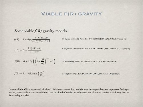
L DARK ENERGY MODEL AND BEHAVIOUR OF ITS FRW SOLUTIONS
(1 + x 2n
1
λ =
)2
g from (1) can be written
x 2n−1
, (17)
1 (2
in
+
the
2x 2n
1following − 2n)
Einsteinian form (though gravity itself is not the
where x 1 = R 1 /R c . From the stability condition 0 <
Rµ ν − 1 (
Viable
)
f(r) gravity
m(r = −2) ≤ 1weobtain
2 δν µR = −8πG Tµ(m) ν + T µ(DE)
ν (2)
2x 4n
1 − (2n − 1)(2n +4)x 2n
1 +(2n − 1)(2n − 2) ≥ 0 .(18)
1
When n = 1,
≡ F ′ (R)Rµ ν − 1 for example,
2
Some F (R)δν µ + ( we have x 1 ≥ √ 3 and
λ ≥ 8 √ 3/9. Under Eq. (18) one
∇ µ ∇ ν can
−I. show
δµ∇ ν FORMULAE that
ρ ∇ ρ) F ′ the condition
(4) is satisfied. This situation is similar to the
(R) , F(R) ≡ f(R) − R (3)
Starobinsky’s model (12),
viable
see Ref.
f(R)
[15]
gravity
for details.
models 1
riation We can of Lextend m and the satisfies abovethe twogeneralized models to the conservation more gen-laeral FORMULAE
andform
the right-hand side of Eq. c 1
Tµ;ν(m) ν =0separately(since
) (3) (R/R satisfythiscondition,too).Thereexistsasubtletyin
HS ) n
discussed below. f(R) The =R trace − R HS ofc 2
Eq. (R/R (2)reads HS ) n +1 , f(R) =R + Rn (aR n − b)
W. Hu and I. Sawicki, Phys.
1+cR n . Rev. D 76 064004 (2007), arXiv:0705.1158[astro-ph]
(1)
f(R) =R − ξ(R), ξ(0) = 0, ξ(R ≫ R c ) → const. (19)
3∇ µ ∇ µ f ′ − Rf ′ +2f =8πGT m . (4)
RThe HS ) n conditions
ns (de Sitter ones for R>0) are roots of the algebraic equation Rf ′ =2f.
S) n +1 , f(R) (4) =R translate + Rn (aR into n − b)
1+cR n . (1)
following3-parametricform:
ξ ,R < 1 , ξ ,RR < 0 , for R ≥ R 1 . (20)
(
In order to satisfy LGC, we require ( that ξ(R) ) −n approaches
aconstantrapidlyasR f(R) =R + λR grows 0 1+ in the R2
R0
2 region− R1)
≫ R c A. Starobinsky, JETP Lett. 86 157 (2007),(5)
arXiv:0706.2041 [astro-ph]
(such as ξ(R) ≃ constant − (R c /R) 2n discussed above).
Another model to meet these requirements is
the order of the presently observed
(
effective cosmological constant. Thenf(0) = 0 (the
appears’ in flat space-time) and Rµ ν ) R =0isalwaysasolutionofEq. (2)intheabsence
gative – flat
f(R)
space-time
=R −
is
λR
unstable. c tanh
For
,
|R| ≫ R 0 ,
(21) S. Tsujikawa, Phys. Rev. D 77 023507 (2008), arXiv:0709.1391[astro-ph]
R c
f(R) =R − 2Λ(∞) where the highctive
cosmological constant is Λ(∞) =λR 0 /2. The equation for de Sitter solutions having
1 where > 0canbewrittenintheform
λ and R c are positive constants. A similar model
was proposed by Appleby and Battye [16], although it is
different from (21) in the sense x 1 (1 + that x 2
λ =
1) ξ(R) n+1 canbenegative
for R < In Rsome limit, 2((1+x GR is 2 1 )n+1 recovered, − 1 − (n the +1)x local 2 1 violations ) . are avoided, and the non-linear (6)
1 . In the region R ≫ R c the model (21)
part become important for large
scales, also avoids matter instabilities...but this kind of models usually cross the phantom barrier, which may lead to
themaximal root of Eq. (6). So, instead of specifying λ, onemaytakeanyvalueofx
future singularities.
1
rresponding value of λ. It follows from the structure of Eq. (6) that x 1 < 2λ. Thus, the
tant at the de Sitter solution Λ(R 1 )=R 1 /4 < Λ(∞). On the other hand, x 1 → 2λ in both
1andx 1 ≫ 1, n fixed. In these cases the Universe evolution becomes indistinguishable
odel.
S. Nojiri and S.D. Odintsov, Phys. Rev. D 77 026007 (2008), arXiv:0710.1738[hep-th]