sbornÃk
sbornÃk sbornÃk
Petr Kahánek, Alexej Kolcun of this deformation is a structured mesh. It is obvious (and important) that it is topologically equivalent to the original grid. Structured triangulation is a structured mesh, whose elements (quadrilaterals) were triangulated, i.e. for every element, one of the two possible diagonals was chosen. There is one great advantage of a structured mesh – we can obtain very efficient form of the incidence matrix of structured mesh. The incidence matrix of nodes plays a significant role for most kinds of simulations. It depends on the manner of node indexing. Fig.4 shows incidence matrix of the regular grid, where nodes are indexed a) randomly, b) in the “spiral way from the boundary to the interior” c) in the “natural way – row by row”. We can see that the last method gives us the best form of the incidence matrix, where all nonzero elements are concentrated in the regular structure near the main diagonal. As a result, use of a structured mesh allows us to solve much larger problems (in terms of number of points), because effective methods for storage and manipulations with incidence matrix are offered in this case [2, 3]. Figure 3: Incidence matrices for different indexing of nodes On the other hand, there is a disadvantage, too: structured meshes are not suitable for refinement. However, the technique of nested meshes can solve this problem (Multigrid methods which use this idea are used for PDE solving) [3]. 4 Structured triangulations with defined geometry Before any calculations can be done, it is neccesary to deform the mesh so that it respects the geometry inherent to the given problem. In general, such geometry can be very complicated; it is, however, a common task to model some basic shapes, i.e. curves in 2D, surfaces in 3D. Here, we will deal with the simplest curve type in two dimensions, line segment. 98
BRESENHAM'S REGULAR MESH DEFORMATION AND... Start in I 1 Until we have reached I 2 Find indices x, y of the next node (via Bresenham) Move it so that it lies on the line If both x and y have changed (in Bresenham) Force corresponding diagonal Algorithm 1: Local mesh deformation There are different ways of mesh deformation [2, 3]. Usually, mesh generators use some kind of parametrization; they, in fact, divide the mesh into several smaller meshes, which are "glued" together with the modelled boundary. Let us suppose that we have a line segment, whose ends are fixed in nodes of the original (not yet deformed) mesh, say I 1 and I 2 . For the process of deformation, we will use an adaptation of the well-known Bresenham's algorithm. We will use it to find out which nodes should be moved during deformation. See Algorithm 1. It is important to say that we move nodes only in direction of one axis (x or y). This is determined by slope α of the given line: for 0 ≤ α ≤ π /4, we will move the nodes only vertically, for π /4
- Page 48 and 49: ÔÖØÓÑØÓÔÓÝÙ×ÓÙÖÓÚ
- Page 50 and 51: Bohumír Bastl The second reason fo
- Page 52 and 53: Bohumír Bastl 4 3 2 1 0 2 4 0 2 4
- Page 54 and 55: Bohumír Bastl the package that bot
- Page 56 and 57: Zuzana Benáková x B y z B B = u c
- Page 58 and 59: Zuzana Benáková Obrázek 4: třet
- Page 60 and 61: Michal Benes Since des t 2 = ds 2 +
- Page 62 and 63: Michal Benes The latter condition i
- Page 64 and 65: Michal Benes 4 Innitesimal deformat
- Page 66 and 67: Michal Benes where , 1, 2, ¢1, ¢2
- Page 68 and 69: Milan Bořík, Vojtěch Honzík sys
- Page 70 and 71: Milan Bořík, Vojtěch Honzík Dá
- Page 72 and 73: Milan Bořík, Vojtěch Honzík Obr
- Page 74 and 75: Jaromír Dobrý Example 2 Let’s c
- Page 76 and 77: Jaromír Dobrý M ϕ ϕ(M) ϑ V {o}
- Page 78 and 79: Jaromír Dobrý It is obvious from
- Page 80 and 81: Henryk Gliński distortion coeffici
- Page 82 and 83: Henryk Gliński polynomial. The coe
- Page 84 and 85: ÊÓÑÒÀõ ÎÖÚÑÓúÒÓÔÖÓ
- Page 86 and 87: ÊÓÑÒÀõ ÃõÒÐÓÝ´ÚÞÇÖ
- Page 88 and 89: ÊÓÑÒÀõ ÈÖÓÖÑÓÒ ÒÑÞ
- Page 90 and 91: Oldřich Hykš foundations and simp
- Page 92 and 93: Oldřich Hykš The choice of the tr
- Page 94 and 95: Oldřich Hykš discussed together w
- Page 96 and 97: Petr Kahánek, Alexej Kolcun 2 Tria
- Page 100 and 101: Petr Kahánek, Alexej Kolcun Now we
- Page 102 and 103: Petr Kahánek, Alexej Kolcun In the
- Page 104 and 105: Mária Kmeťová Bernsteinove polyn
- Page 106 and 107: Mária Kmeťová H 0 O H 1 V 1 V 2
- Page 108 and 109: Mária Kmeťová Na obrázku 5 je k
- Page 110 and 111: Mária Kmeťová 6 Záver Program E
- Page 112 and 113: Milada Kočandrlová Pro body X eli
- Page 114 and 115: Milada Kočandrlová Podmínku cykl
- Page 116 and 117: Milada Kočandrlová 6 Homotetický
- Page 118 and 119: Jiří Kosinka medial axis transfor
- Page 120 and 121: Jiří Kosinka Figure 3: Asymptotic
- Page 122 and 123: Jiří Kosinka a) b) Figure 4: a) F
- Page 124 and 125: Iva Křivková • body (např. Bri
- Page 126 and 127: Iva Křivková V trojrozměrném eu
- Page 128 and 129: Iva Křivková asymptoty). V tomto
- Page 130 and 131: Karolína Kundrátová myslíme roz
- Page 132 and 133: Karolína Kundrátová Bázové fun
- Page 134 and 135: Karolína Kundrátová Obr. 2: Kři
- Page 136 and 137: Miroslav Lávička of this article
- Page 138 and 139: Miroslav Lávička if 〈x, x〉 M
- Page 140 and 141: Miroslav Lávička n: x - x = 0 0 4
- Page 142 and 143: Miroslav Lávička 5 Conclusion In
- Page 144 and 145: Pavel Leischner Věta 1 (ptolemaiov
- Page 146 and 147: Pavel Leischner Věta 2 (Ptolemaiov
BRESENHAM'S REGULAR MESH DEFORMATION AND...<br />
Start in I 1<br />
Until we have reached I 2<br />
Find indices x, y of the next node (via<br />
Bresenham)<br />
Move it so that it lies on the line<br />
If both x and y have changed (in Bresenham)<br />
Force corresponding diagonal<br />
Algorithm 1: Local mesh deformation<br />
There are different ways of mesh deformation [2, 3]. Usually, mesh<br />
generators use some kind of parametrization; they, in fact, divide the mesh<br />
into several smaller meshes, which are "glued" together with the modelled<br />
boundary.<br />
Let us suppose that we have a line segment, whose ends are fixed in<br />
nodes of the original (not yet deformed) mesh, say I 1 and I 2 . For the process<br />
of deformation, we will use an adaptation of the well-known Bresenham's<br />
algorithm. We will use it to find out which nodes should be moved during<br />
deformation. See Algorithm 1.<br />
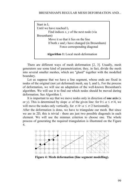
It is important to say that we move nodes only in direction of one axis (x<br />
or y). This is determined by slope α of the given line: for 0 ≤ α ≤ π /4, we<br />
will move the nodes only vertically, for π /4


