- Page 1 and 2: Katedra matematiky Fakulty stavebn
- Page 3 and 4: Programový výbor konference: Doc.
- Page 5: OBSAH TABLE OF CONTENTS
- Page 8 and 9: Table of Contents Petr Kahánek, Al
- Page 10 and 11: Table of Contents Daniela Velichov
- Page 13: PLENÁRNÍ PŘEDNÁŠKY PLENARY LEC
- Page 16 and 17: František Kuřina sítě čtyřdim
- Page 18 and 19: František Kuřina Kombinace těcht
- Page 20 and 21: František Kuřina 3 Matematika a v
- Page 22 and 23: František Kuřina řešení je alt
- Page 24 and 25: Gunter Weiss should show an own sci
- Page 26 and 27: Gunter Weiss “industrial reality
- Page 28 and 29: Gunter Weiss 5 “e-learning Geomet
- Page 30 and 31: Gunter Weiss In the following some
- Page 32 and 33: Gunter Weiss screen. This made it f
- Page 35: REFERÁTY CONFERENCE PAPERS
- Page 38 and 39: Eva Baranová, Kamil Maleček S a a
- Page 40 and 41: Eva Baranová, Kamil Maleček extr
- Page 42 and 43: Eva Baranová, Kamil Maleček Obrá
- Page 44 and 45: ÊÓÞÔ×ÑÓ×ÓÙÖÒÔÞ×Ñ Å
- Page 46 and 47: ÞÓÓÑÓÒÒ×ÓÙÖÒ×ÓÙÊ´
- Page 48 and 49: ÔÖØÓÑØÓÔÓÝÙ×ÓÙÖÓÚ
- Page 50 and 51: Bohumír Bastl The second reason fo
- Page 54 and 55: Bohumír Bastl the package that bot
- Page 56 and 57: Zuzana Benáková x B y z B B = u c
- Page 58 and 59: Zuzana Benáková Obrázek 4: třet
- Page 60 and 61: Michal Benes Since des t 2 = ds 2 +
- Page 62 and 63: Michal Benes The latter condition i
- Page 64 and 65: Michal Benes 4 Innitesimal deformat
- Page 66 and 67: Michal Benes where , 1, 2, ¢1, ¢2
- Page 68 and 69: Milan Bořík, Vojtěch Honzík sys
- Page 70 and 71: Milan Bořík, Vojtěch Honzík Dá
- Page 72 and 73: Milan Bořík, Vojtěch Honzík Obr
- Page 74 and 75: Jaromír Dobrý Example 2 Let’s c
- Page 76 and 77: Jaromír Dobrý M ϕ ϕ(M) ϑ V {o}
- Page 78 and 79: Jaromír Dobrý It is obvious from
- Page 80 and 81: Henryk Gliński distortion coeffici
- Page 82 and 83: Henryk Gliński polynomial. The coe
- Page 84 and 85: ÊÓÑÒÀõ ÎÖÚÑÓúÒÓÔÖÓ
- Page 86 and 87: ÊÓÑÒÀõ ÃõÒÐÓÝ´ÚÞÇÖ
- Page 88 and 89: ÊÓÑÒÀõ ÈÖÓÖÑÓÒ ÒÑÞ
- Page 90 and 91: Oldřich Hykš foundations and simp
- Page 92 and 93: Oldřich Hykš The choice of the tr
- Page 94 and 95: Oldřich Hykš discussed together w
- Page 96 and 97: Petr Kahánek, Alexej Kolcun 2 Tria
- Page 98 and 99: Petr Kahánek, Alexej Kolcun of thi
- Page 100 and 101: Petr Kahánek, Alexej Kolcun Now we
- Page 102 and 103:
Petr Kahánek, Alexej Kolcun In the
- Page 104 and 105:
Mária Kmeťová Bernsteinove polyn
- Page 106 and 107:
Mária Kmeťová H 0 O H 1 V 1 V 2
- Page 108 and 109:
Mária Kmeťová Na obrázku 5 je k
- Page 110 and 111:
Mária Kmeťová 6 Záver Program E
- Page 112 and 113:
Milada Kočandrlová Pro body X eli
- Page 114 and 115:
Milada Kočandrlová Podmínku cykl
- Page 116 and 117:
Milada Kočandrlová 6 Homotetický
- Page 118 and 119:
Jiří Kosinka medial axis transfor
- Page 120 and 121:
Jiří Kosinka Figure 3: Asymptotic
- Page 122 and 123:
Jiří Kosinka a) b) Figure 4: a) F
- Page 124 and 125:
Iva Křivková • body (např. Bri
- Page 126 and 127:
Iva Křivková V trojrozměrném eu
- Page 128 and 129:
Iva Křivková asymptoty). V tomto
- Page 130 and 131:
Karolína Kundrátová myslíme roz
- Page 132 and 133:
Karolína Kundrátová Bázové fun
- Page 134 and 135:
Karolína Kundrátová Obr. 2: Kři
- Page 136 and 137:
Miroslav Lávička of this article
- Page 138 and 139:
Miroslav Lávička if 〈x, x〉 M
- Page 140 and 141:
Miroslav Lávička n: x - x = 0 0 4
- Page 142 and 143:
Miroslav Lávička 5 Conclusion In
- Page 144 and 145:
Pavel Leischner Věta 1 (ptolemaiov
- Page 146 and 147:
Pavel Leischner Věta 2 (Ptolemaiov
- Page 148 and 149:
Pavel Leischner Literatura [1] Enge
- Page 150 and 151:
Ivana Linkeová Je-li hodnota výra
- Page 152 and 153:
Ivana Linkeová jednotkové váhy.
- Page 154 and 155:
Ivana Linkeová funkce jsou pro u 0
- Page 156 and 157:
Dalibor Martišek systémech, je po
- Page 158 and 159:
Dalibor Martišek Zvládneme-li pra
- Page 160 and 161:
Dalibor Martišek (což je jednoduc
- Page 162 and 163:
Katarína Mészárosová vedcov nov
- Page 164 and 165:
Katarína Mészárosová Obrázok 1
- Page 166 and 167:
Katarína Mészárosová Analogicky
- Page 168 and 169:
Katarína Mészárosová pocit krá
- Page 170 and 171:
Martin Němec do databáze, popří
- Page 172 and 173:
Martin Němec Obrázek 3: Modul pro
- Page 174 and 175:
Martin Němec Literatura [1] J. Ziv
- Page 176 and 177:
Stanislav Olivík 2 Hledání odraz
- Page 178 and 179:
Stanislav Olivík S 1 Q i+2 P Q Q i
- Page 180 and 181:
Stanislav Olivík Metoda popsaná v
- Page 182 and 183:
Anna Porazilová Table 1 shows the
- Page 184 and 185:
Anna Porazilová respective sum of
- Page 186 and 187:
Anna Porazilová Figure 4a. Demonst
- Page 188 and 189:
Anna Porazilová precisely (figure
- Page 190 and 191:
LenkaPospíšilová výpočtupřija
- Page 192 and 193:
LenkaPospíšilová > evolute:=proc
- Page 194 and 195:
LenkaPospíšilová Soustavatečenp
- Page 196 and 197:
Radka Pospíšilová Pro získání
- Page 198 and 199:
Radka Pospíšilová Obrázek 2: Uk
- Page 200 and 201:
Jana Procházková 2 Derivative of
- Page 202 and 203:
Jana Procházková now we continue
- Page 204 and 205:
Jana Procházková Figure 1: Tangen
- Page 206 and 207:
Marie Provazníková SO(n) je topol
- Page 208 and 209:
Marie Provazníková qiq −1 = −
- Page 210 and 211:
Marie Provazníková Potom máme do
- Page 212 and 213:
Jana Přívratská ponechává nedo
- Page 214 and 215:
Jana Přívratská Z 16 klasických
- Page 216 and 217:
Adam Rużyczka During those years,
- Page 218 and 219:
Adam Rużyczka % 100 90 80 70 60 50
- Page 220 and 221:
Adam Rużyczka Table 3 presents com
- Page 222 and 223:
Ivo Serba Obr. 1. Princip geometric
- Page 224 and 225:
Ivo Serba výplň rohů = vloop( vp
- Page 226 and 227:
Ivo Serba . Obr. 7. Příklad tří
- Page 228 and 229:
Ivo Serba Literatura [1] Cline, M.:
- Page 230 and 231:
Tomáš Staudek vizualizací prosto
- Page 232 and 233:
Tomáš Staudek - Matematické mode
- Page 234 and 235:
Tomáš Staudek - Stíny (měkké,
- Page 236 and 237:
Zbyněk Šír circular arcs share o
- Page 238 and 239:
Zbyněk Šír In addition to the hi
- Page 240 and 241:
JiříŠrubař Jetakézřejmé,žen
- Page 242 and 243:
JiříŠrubař cházejícístředys
- Page 244 and 245:
JiříŠrubař |LS|=|OS|, |TS|= 1 2
- Page 246 and 247:
Diana Šteflová 2 Digitální foto
- Page 248 and 249:
Diana Šteflová Organizační prav
- Page 250 and 251:
Vladimír Tichý Definice a označe
- Page 252 and 253:
Vladimír Tichý Případy 2 až 4
- Page 254 and 255:
Vladimír Tichý V tomto konkrétn
- Page 256 and 257:
Světlana Tomiczková Figure 1: Are
- Page 258 and 259:
Světlana Tomiczková follows: 1. B
- Page 260 and 261:
Světlana Tomiczková ∫ [x 2 (s(t
- Page 262 and 263:
Margita Vajsáblová Křovák zostr
- Page 264 and 265:
Margita Vajsáblová 3 Použitie ku
- Page 266 and 267:
Margita Vajsáblová Obrázok 4: Gr
- Page 268 and 269:
Jiří Vaníček technického směr
- Page 270 and 271:
Jiří Vaníček Vzhledem k nasazen
- Page 272 and 273:
Jiří Vaníček politiky a má zvy
- Page 274 and 275:
Jiří Vaníček tedy které úlohy
- Page 276 and 277:
Jana Vecková 2 Algoritmus navrhova
- Page 278 and 279:
Jana Vecková Obrázek 5: Porovnán
- Page 280 and 281:
Daniela Velichová 2 Dvojosové rot
- Page 282 and 283:
Daniela Velichová Obrázok 3: Dvoj
- Page 284 and 285:
Daniela Velichová Skupina IB1 - Cy
- Page 286 and 287:
Daniela Velichová Parametrické ro
- Page 288 and 289:
Šárka Voráčová also available
- Page 290 and 291:
Šárka Voráčová efficiency is p
- Page 292 and 293:
Šárka Voráčová 5 Conclusion Ma
- Page 294 and 295:
Edita Vranková (intM∩intN=∅).
- Page 296 and 297:
Edita Vranková translations). This
- Page 298 and 299:
Edita Vranková From all previous s
- Page 300 and 301:
Edita Vranková References [1] Bíl
- Page 302 and 303:
Radek Výrut Další postup využí
- Page 304 and 305:
Radek Výrut Nyní si podrobněji p
- Page 306 and 307:
Radek Výrut [3] I. K. Lee, M. S. K
- Page 308 and 309:
Lucie Zrůstová Náplň deskriptiv
- Page 310 and 311:
Lucie Zrůstová V roce 1951 byla z
- Page 312 and 313:
Lucie Zrůstová Školní rok Zimn
- Page 314 and 315:
Mária Zvariková, Zuzana Juščák
- Page 316 and 317:
Mária Zvariková, Zuzana Juščák
- Page 318 and 319:
Mária Zvariková, Zuzana Juščák
- Page 320 and 321:
Antonina Żaba An attempt to find a
- Page 322 and 323:
Antonina Żaba Figure 2: Drawing fr
- Page 324 and 325:
Antonina Żaba element) are include
- Page 326 and 327:
Antonina Żaba but look slantwise a
- Page 328 and 329:
Antonina Żaba Figure 2: Drawing 56
- Page 330 and 331:
Antonina Żaba In S. Ignazio Church
- Page 333 and 334:
25. KONFERENCE O GEOMETRII A POČÍ
- Page 335 and 336:
Seznam účastníků Milena Foglaro
- Page 337 and 338:
Alexej Kolcun Akademie věd České
- Page 339 and 340:
Seznam účastníků Dagmar Mannhei
- Page 341 and 342:
Seznam účastníků Radka Pospíš
- Page 343 and 344:
Seznam účastníků Jaroslav Škra
- Page 345 and 346:
Edita Vranková Trnavská univerzit
- Page 347:
ELKAN, spol. s r.o. Výhradní dist