Python algorithms in particle tracking microrheology - Chemistry ...

Maier and Haraszti Chemistry Central Journal 2012, 6:144 

http://journal.chemistrycentral.com/content/6/1/144 

SOFTWARE 

Open Access 

Python algorithms in particle tracking 

microrheology 

Timo Maier 1,2 and Tamás Haraszti 1,2* 

Abstract 

Background: Particle tracking passive microrheology relates recorded trajectories of microbeads, embedded in soft 

samples, to the local mechanical properties of the sample. The method requires intensive numerical data processing 

and tools allowing control of the calculation errors. 

Results: We report the development of a software package collecting functions and scripts written in Python for 

automated and manual data processing, to extract viscoelastic information about the sample using recorded particle 

trajectories. The resulting program package analyzes the fundamental diffusion characteristics of particle trajectories 

and calculates the frequency dependent complex shear modulus using methods published in the literature. In order 

to increase conversion accuracy, segmentwise, double step, range-adaptive fitting and dynamic sampling algorithms 

are introduced to interpolate the data in a splinelike manner. 

Conclusions: The presented set of algorithms allows for flexible data processing for particle tracking microrheology. 

The package presents improved algorithms for mean square displacement estimation, controlling effects of frame loss 

during recording, and a novel numerical conversion method using segmentwise interpolation, decreasing the 

conversion error from about 100% to the order of 1%. 

Keywords: Particle tracking microrheology, Numerical conversion method, Software library, Dynamic interpolation 

Background 

Particle tracking microrheology is a modern tool to investigate 

the viscoelastic properties of soft matter, for example, 

biopolymers and the interior, or the membrane of 

living cells [1,2] on the microscopic scale. Though embedding 

tracer particles into such a sample alters the local 

structure, this method is still considered non-invasive and 

provides important information not available by other 

methods [1-4]. 

The physical background of the method lies in the thermal 

motion of the tracer particle, which can be connected 

to the viscoelastic properties of the local environment 

through the generalized Langevin equation [5,6]. Neglecting 

the inertia term, which contributes to frequencies 

in the megahertz range, and assuming that the memory 

function is linearly related to the frequency dependent 

*Correspondence: tamas.haraszti@uni-heidelberg.de 

1 Max-Planck Institute for Intelligent Systems, Advanced Materials and 

Biosystems, Heisenberg str. 3, 70569 Stuttgart, Germany 

2 Biophysical Chemistry, Institute of Physical Chemistry, University of 

Heidelberg, Im Neuenheimer Feld 253, 69120 Heidelberg, Germany 

viscosity of the medium (through a generalized Stokes- 

Einstein relation)[3,5-8], the mean square displacement 

(MSD) of the particle can be directly related to the creep 

compliance as: 

J(τ) = 

3 πa 

N D k B T , (1) 

where τ denotes the time step in which the particle moves 

r distance, the mean square displacement, 

N D the dimensionality of the motion (usually N D = 2for 

particle tracking digital microscopy), k B the Boltzmann 

constant, T is the absolute temperature and a the particle 

radius, respectively. 

Active microrheology (using optical or magnetic tweezers) 

and macroscopic rheometry commonly characterize 

the sample elasticity with the frequency-dependent complex 

shear modulus, G ∗ (ω), which is a complex quantity 

[4,9,10]. Its real part is known as the storage modulus 

G ′ (ω) and the imaginary part is the loss modulus, G ′′ (ω). 

While J(t) is a description in the time domain, G ∗ (ω) is 

an equivalent characterization in the frequency domain. 

© 2012 Maier and Haraszti; licensee Chemistry Central Ltd. This is an Open Access article distributed under the terms of the 

Creative Commons Attribution License (http://creativecommons.org/licenses/by/2.0), which permits unrestricted use, 

distribution, and reproduction in any medium, provided the original work is properly cited.

Maier and Haraszti Chemistry Central Journal 2012, 6:144 Page 2 of 9 


The two types of description are equivalent and interconnected 

with the relation: 

G ∗ (ω) = 1 

iω˜J(ω) , (2) 

where ˜J(ω) is the Fourier transform of J(t). Assuming that 

the particle tracks are previously obtained, the frequency 

dependent complex shear modulus G ∗ (ω) can be derived 

using equations (1) and (2) after calculating the mean 

square displacement. 

There are two major algorithm libraries available on the 

Interned addressing data handling for microrheology: the 

algorithm collection of J. Crocker et al. written in the 

interactive data language (IDL) [11], which was translated 

to Matlab and expanded by the Kilfoil lab [12]. A separate 

stand alone algorithm is provided by M. Tassieri for 

calculating the complex shear modulus from the creep 

compliance, written in LabView [13]. However, an extensible 

integrated framework relying on freely accessible 

software and source code integrating multiple conversion 

methods is not yet available. 

In this paper we present a software package written in 

the interpreted programing language Python (http://www. 

python.org) collecting functions to support particle tracking 

microrheology related calculations, with emphasis on 

those parts providing enhanced functionality. This library 

is meant to be an open source, platform independent, 

freely extendable set of algorithms allowing to extract 

rheology information from particle tracks obtained 

previously. 

The Rheology software library contains two example 

scripts. One called ProcessRheology.py, a configuration 

driven program performing all processing steps from particle 

trajectory inputs, thus presenting the various capabilities 

of the library (Figure 1). This program can be 

employed as a self-standing calculator or its code can 

be used as a template for the user testing the Rheology 

library. The other is the Function-test.py, containing test 

calculations, and which was also employed to produce the 

figures in this article (see the content of the Additional 

file 1). 

Implementation 

Dependencies 

The software depends on the following Python packages 

for calculations and displaying results: 

• Numpy: a library for array manipulation and 

calculations [14]; 

• Scipy: the Python scientific library, from which we 

used the gamma function and the nonlinear least 

squares fitting function [14]; 

• Matplotlib: a Matlab-like plotting library to generate 

information graphs of the results [15]. 

Figure 1 Process flow chart of microrheology data. The 

fundamental processing steps in particle tracking microrheology as 

followed by the ProcessRheology.py script. There are several 

parameters that may affect the details of the process, including the 

sampling in the MSD calculation and which way the complex shear 

modulus is calculated (see the main text for details). In this article we 

focus mainly on the later tree steps in the process: the MSD 

calculation and conversion methods. 

After installation, its functions are available using following 

import command within the interpreter or a 

Python script: 

from Rheology import * 

Data presentation, data format 

Instead of defining individual classes for each data type 

(MSD, creep compliance and complex shear modulus), an 

alternative technique in Python is to employ generalized 

lists, the so called dictionaries or ‘dicts’. A dict is a container 

class holding data which are indexed with arbitrary 

keys (marked by quotes in this paper). This is a very general 

and flexible data structure, which we used for all data 

in the Rheology package. For example, MSD dicts contain 

keys “tau” and “MSD” referring to arrays holding the time 

lag and the mean square displacement data, respectively. 

Particle trajectories 

Particle tracking microrheology starts with the imaging 

experiments and the image treatment in a strict



sense, however, obtaining particle trajectories from video 

microscopy is well described in the literature [16-20] 

including the statistical difficulties of the process [21-23]. 

There are various implementations of particle tracking 

algorithms available in IDL (see the same website as 

for the rheology code) [11,24], Matlab [12,25], LabView 

[20,26] or C++ languages [27]. An implementation of the 

Grier method [16] is also translated to Python [28]. 

Thus, we start our discussion by extracting rheological 

information from the particle trajectories, leaving the 

implementation of data input/output to the user. As a 

good starting template, we recommend the ReadTable() 

and SaveTable() functions in the ProcessRheology.py example 

script. 

Drift correction 

Several experimental systems show a drift: a slow oriented 

motion of the sample versus the imaging frame, which is 

caused by various factors of the experimenting apparatus. 

To remove this drift, which is independent of the sample, 

there are multiple possibilities one may consider. If a 

reference bead bound to the sample is available, its trajectory 

provides the drift itself. If multiple particles are 

tracked in the same time interval, an average trajectory 

may be calculated and used as a reference. If these possibilities 

are not available, one has to consider whether 

the long time motion is due to drift or it is a characteristic 

of the investigated sample, because subtracting it 

changes the resulted long time lag (low frequency) part of 

the viscoelastic characteristics. 

The simplest way of data treatment in such cases is 

to calculate a smoothened trajectory: e. g. using a running 

average, and either subtract this smoothened data 

or, in one further step, fit a low order polynomial to the 

smoothened data and subtract the fitted values from the 

trajectory. 

A very simple implementation is available for two 

dimensional data sets as: 

GetData(timestamps, poslist, indx=0, 

order=3,resolution=0.1434, Nd= 1000) 

This algorithm takes a position list (parameter poslist), 

which is a list of dicts, each describing the positions of a 

particle. The indx parameter is used to select one of them. 

A position dict contains “X”, and “Y”, which are arrays of 

the x and y positions.Thedictalsocontainsanindex 

array denoted with key “indx”, identifying the image index 

(serial number) of the given positions. Using this index 

allows the tracking algorithm to miss individual frames (e. 

g. when the particle drifted out of focus). This index is also 

used to define the time point of a position, either by identifying 

the corresponding time stamps, provided in seconds 

in the timestamps array, or if this variable is set to None, 

multiplying the index by the optional tscale parameter. 

The Nd parameter gives the number of points used in the 

running average and the order parameter identifies the 

order of the polynomial to be fitted for drift correction. If 

Nd is set to −1, the running averaging is off, and if order is 

-1, the drift correction is turned off. The resolution is used 

to scale the coordinates to micrometers (the same value 

for both coordinates). 

Mean square displacement (MSD) 

Characterizing a soft sample using particle tracking 

microrheology strongly relies on the determination of 

the mean square displacement. Calculating the MSD has 

two possible sets of assumptions: 1.) ensemble averages 

are based on recording many tracer particles and assuming 

homogeneity across the sample. This is the averaging 

method considered in theories, and has the advantage 

allowing estimation of the time-dependent aging of the 

system. Technically this can be achieved by using video 

recording-based particle tracking, where the number of 

tracers can be increased to the order of tens. 2.) Assuming 

ergodicity, one can switch from ensemble averaging to 

time averaging. This is very important for systems which 

are not homogeneous and for cases where only few particles 

(1 − 5) can be observed at a time. For samples of 

biological origin, time averaging is more suitable because 

these samples are seldom homogeneous. 

Calculating the time average is done by splitting up the 

trajectory into non-overlapping parts and averaging their 

displacement.Becausethenumberofintervalsdecreases 

with an increasing lag time, this method has very high 

error for large lag time values. Alternatively, it is also possible 

to split the trajectory into overlapping regions and 

then do the averaging. The resulting statistical errors follow 

a non-normal distribution, but it has been shown that 

using overlapping segments the resulted MSD may show 

improved accuracy [29,30] when using lag time values up 

to about the quarter of the measurement length (N/4 for 

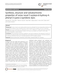
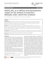
N data points). The results of a test calculation using positions 

randomly calculated from a normal distribution with 

standard deviation of σ X = σ Y = 0.15 μm in both X and 

Y directions are presented in Figure 2. The MSD oscillates 

around the theoretical value of = 2(σ 2 X + 

σ 2 Y ) = 0.09 μm2 as expected, but the data calculated using 

overlapping intervals show visibly better accuracy. 

msd = MSD(positionlist, tau= 0) 

MSD() is the function to calculate the mean square displacement 

from a single trajectory. The data points are 

presented as a two dimensional array positionlist,containing 

coordinates ((x, y) or (x, y, z)) in each row. 

The second parameter (tau) is used to generate the lag 

time values (steps) for which the MSD is calculated. This



MSD, μm 2 

1 

0.1 

0.01 

0.001 

0.01 0.1 1 10 100 

τ, seconds 

Figure 2 mean square displacement data calculated from 

simulated data. The distribution of X and Y positions were generated 

based on a normal distribution with σ = 0.15 μm. The theoretical 

MSD is constant at 0.09 μm 2 (black line). Data with non-overlapping 

intervals (red + symbols) show higher scattering, the ones calculated 

with overlapping intervals (green ×) show a much lower error. 

parameter can take various values: If an array or list of 

integer values are given, then those are used as index step 

values. If a single integer is given between 0 and the number 

of positions, then so many index steps (lag time values) 

are generated in an equidistant manner. If nothing, or 0 is 

given, then values 1 ...N/4areused. 

Each tau value results in M = M(tau) pairs, where 

the step r[ i + tau] −r[ i]iscalculated.M also depends on 

whether the set was generated using overlapping intervals 

(if overlap = True is set). 

If an array of time values (in seconds) are provided for 

the position data using the optional tvector parameter, the 

algorithm will check the time step between each data pair 

used. Calculating the mean value of these time steps and 

using a relative error, every value outside the mean (1 ± 

tolerance) will be ignored (by default tolerance = 0.1). 

This process eliminates jumps in the data caused by computer 

latency during recording. 

The function returns a dictionary containing “tau”, 

“dtau”,“MSD”,“DMSD”keys.Ifthetimevalueswerenot 

provided, then “tau” holds the index steps between the 

positions and “dtau” is not used. 

Creep compliance 

Assuming that the generalized Stokes-Einstein relation 

holds, the creep compliance is linearly proportional to the 

MSD [6]. The MSD to J() function calculates the creep 

compliance using equation (1). 

J = MSD to J(msd, t0= 0.1, tend= 150, 

T= 25.0, a= 1.0) 

The calculation requires a dict structure (msd) having 

thetimevaluesunderthe“tau”key,andtheMSDvalues 

under the “MSD” key (error values are optional). Further 

parameters are the temperature T of the experiment in 

Celsius degrees, the radius a oftheappliedtracerparticle 

in micrometers, and optionally the dimensionality of the 

motion D (denoted as N D in equation (1)), which is set to 

D = 2 by default. 

Calculating the frequency dependent shear modulus 

from J(t) with the numerical method proposed by Evans 

et al. requires extrapolated values to the zero time point 

and to infinite time values. These values are estimated 

here, allowing the user to override them before being used 

to calculate the complex shear modulus G ∗ (ω). Thezero 

time value J 0 = J(t = 0) is extrapolated from a linear fit 

in the t < t0 region, and the end extrapolation is obtained 

from a linear fit to the tend < t part.Theslopeofthe 

extrapolated end part is 1/η, whereη is the steady state 

viscosity [31]. 

The function returns a new dict containing: “J” (in 

1/Pa), “tau”, “eta”, “J0”, “const”, “dJ”, and the fit parameters 

as “a0”, “b0” for the first part and “a1”, “b1” for the end part, 

where the linear equation J = a i t + b i (i = 0, 1) holds. 

Calculating the frequency dependent complex shear modulus 

While the connection presented by equation (2) is simple, 

there is a major problem with determining ˜J(ω) numerically.Itiswellknowninnumericalanalysisthatapplying 

a numerical Fourier transform increases the experimental 

noise enormously [32]. In microrheology, there are 

four commonly applied methods to solve this problem. 

The first two address the noise of the Fourier transform 

directly by averaging or by fitting, the second two were 

suggested in the last decade to improve the transform 

itself [6,9,31-33]. 

In a homogeneous system, where multiple particles can 

be tracked, converting their MSD to creep compliance and 

then G ∗ (ω) using a discrete Fourier transform, allows one 

to average the converted values and decrease the noise 

this way [32,33]. For cases when the creep compliance can 

be modeled using an analytical form, the Fourier transform 

of the fitted analytical function may be calculated 

and used to estimate of G ∗ (ω) [9]. 

As we have discussed above, samples of biological origin 

are often not homogeneous and their MSD does not follow 

a well-described analytical function. However, model 

calculations suggest, in agreement with experiments, that 

biopolymers and many polymer gels show power law 

behavior at various time ranges [34-36]. The third and 

fourth conversion approaches have been suggested for 

such systems in the microrheology literature. One uses 

a power law approximation of the MSD or the creepcompliance 

[6] (we shall call the Mason method), and the 

other calculates a linear interpolation between the data 

points and applying a discrete Fourier transform on it [31] 

(we shall cite as the Evans method).



Because these methods have their strength and weakness, 

we summarize them and their implementation 

below. Recently we have shown that the accuracy of the 

Evans method can be greatly improved by using local 

interpolation of the data in a splinelike manner without 

forcing a single function to be fitted to the whole data 

set. This improvement is also included in the Rheology 

framework and will be discussed below. 

The Mason method 

This is a fast conversion method based on the Fourier 

transformation of a power function, which has been used 

in various works in the last decade [6-8,37-39]. Briefly, 

let us consider a generalized diffusion process, where the 

MSD is following a power law: < r(t) 2 >= 2N D Dt α 

[40], where D is the generalized diffusion coefficient, and 

0



J 0 and η are already estimated using the linear fits in 

the MSD to J() function. Using equation (5) is straightforward, 

and allow for the calculation of G ∗ (ω) at any ω 

values. The natural selection of a suitable frequency range 

would be from 0 to N 

T π (the unit is 1/s) inN/2 stepsas 

it is common for the discrete Fourier transform of equally 

sampled data [32]. The corresponding function is: 

G = J to G(J) 

The algorithm generates a linear array of frequencies, 

but the number of points is limited to be maximum 1000, 

usually more than sufficient (MSD and creep compliance 

data arrays may hold several thousand points). The result 

is a similar dictionary as it was for the Mason method, 

and can be tested using a Maxwell-fluid, which has a linear 

creep compliance in the form of J(t) = 1/E + t/η 

(Figure 4). 

There are various details worth mentioning about this 

method, which may affect the accuracy of the result in 

general cases. It is clear in equation (5), that the method is 

sensitive to the A k+1 − A k terms, which, in extreme cases, 

may be either very small for a nearly linear part of J(t) or 

very high for sudden jumps in the experimental data. In 

order to reduce round-off errors, one may eliminate the 

closetozerovalues,(when|A k+1 − A k |



1. define the data range using indices i 0 = 0 and 

i 1 = i(t 0 ), containing at least 4 data points; 

2. fit function from i 0 ...i 1 , calculate the squared error 

of each point and estimate the average error; 

3. find the last point around i 1 where χ 2 (i 2 )



100 

Additional file 

G’, G’’, Pa 

10 

1 

Additional file 1: rheology.zip - compressed ZIP archive containing 

the Rheology Python package. The archive contains several files. The 

source code in the Rheology subfolder, a setup.py for installation, 

README.txt and License.txt files and the Example subfolder. Installation (as 

usual in python): 

python setup.py build; python setup.py install 

0.1 

0.01 

0.1 1 10 100 1000 

ω, 1/s 

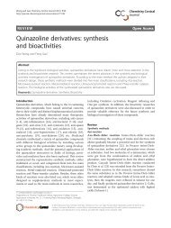
Figure 6 Dynamic resampling. Dynamic resampling can correct the 

errors of the Evans method resulting in an improved fit. The storage 

modulus (red +) and loss modulus (green ×) data calculated 

numerically shows a good fit to the theoretically predicted values 

(black lines). 

The Example subfolder contains two Python scripts. The Function-test.py 

can be used to run test calculations and see the example plots presenting 

that all functions work properly. The figures presented in this paper were 

also generated by this script. 

The ProcessRheology.py is a batch processing script, controlled by 

commands and parameters provided in a config.txt plain text file. An 

example of this file is also included here, containing detailed description of 

every parameter. This scripts is a fully functioning microrheology data 

evaluation toolkit, utilizing the functions of the Rheology package. 

Abbreviations 

MSD, Mean square displacement. 

Competing interests 

The Authors declare that they have not competing interests. 

defined by the NSmooth parameter. The range is identified 

in the original data, but then applied to the refined 

data set. The result is an MSD, where sudden jumps are 

reduced, minimizing the presence of oscillatory artifacts 

in the resulted complex shear modulus G ∗ (ω). 

Conclusions 

Inthispaperwehavepresentedafreesoftwaresolution 

for analyzing particle tracking data for microrheology. 

Our software library implements the time average calculation 

of mean square displacement with control over the 

time shift in the data, and conversion methods to calculate 

the creep compliance and the complex shear modulus. 

Beyond the two most common methods mentioned in the 

literature, we have developed a dynamic local fitting procedure, 

which allows spline-like fitting of the MSD and 

improved conversion accuracy to about 1% from about 

100% for a Kelvin-Voigt model test. 

Availability and requirements 

Lists the following: 

• Project name: Rheology for Python 

• Project home page: http://launchpad.net/ 

microrheologypy/ 

• Operating systems: Platform independent (Linux, 

Windows and Max OSX tested) 

• Programing language: Python 2.7 

• Other requirements: Numpy 1.5, Scipy 0.1, 

Matplotlib 1.0 

• License: LGPL v3 

• Any restrictions to use by non-academics: see 

license 

Authors’ contributions 

TM and TH have developed the Python software together discussing and 

testing the various features, and both contributed to writing this manuscript. 

Both authors read and approved the final manuscript. 

Acknowledgements 

This work was supported by the Ministry of Science, Research, and the Arts of 

Baden-Württemberg (AZ:720.830-5-10a). The authors would like to thank to 

Professor Dr. Joachim P. Spatz, Dr. Heike Boehm and the Max-Planck Society 

for the generous financial support and Dr. Claire Cobley for assistance. 

Received: 13 September 2012 Accepted: 14 November 2012 

Published: 27 November 2012 

References 

1. Dangaria JHH, Butler PJJ: Macrorheology and adaptive microrheology 

of endothelial cells subjected to fluid shear stress. Am J Physiol Cell 

Physiol 2007, 293:C1568—C1575. 

2. Bausch AR, Moller W, Sackmann E: Measurement of local viscoelasticity 

and forces in living cells by magnetic tweezers. Biophys J 1999, 

76:573–579. 

3. Waigh TA: Microrheology of complex fluids. Rep Prog Phys 2005, 

68(3):685. 

4. Wirtz D: Particle-tracking microrheology of living cells: principles 

and applications. Annu Rev Biophys 2009, 38:301–326. 

5. Mason TG, Weitz DA: Optical measurements of frequency-dependent 

linear viscoelastic moduli of complex fluids. Phys Rev Lett 1995, 

74(7):1250–1253. 

6. Mason TG, Ganesan K, van Zanten JH, Wirtz D, Kuo SC: Particle tracking 

microrheology of complex fluids. Phys Rev Lett 1997, 79:3282 – 3285. 

7. Mason TG: Estimating the viscoelastic moduli of complex fluids using 

the generalized Stokes-E, instein equation. Rheologica Acta 2000, 

39(4):371–378. 

8. Squires TM, Mason TG: Fluid mechanics of microrheology. Annu Rev 

Fluid Mech 2010, 42:413–438. 

9. Goodwin JW, Hughes RW: Rheology for Chemists. An Introduction.Second 

edition. Cambridge: RSC Publishing; 2008. 

10. Mezger TG: The Rheology Handbook. 3rd revised edition. Vincentz Network 

GmbH & Co. KG , Plathnerstr. 4c, Vol. 30175. Hannover, Germany: European 

Coatings Tech Files, Vincentz Network; 2011. 

11. Crocker J, Weeks E: Microrheology tools for IDL . [http://www.physics. 

emory.edu/weeks/idl/rheo.html]



12. Kilfoil M, et al.: Matlab algorithms from the Kilfoil lab. [http://people. 

umass.edu/kilfoil/downloads.html] 

13. Tassieri M: Compliance to complex moduli, version 2. 2011. [https:// 

sites.google.com/site/manliotassieri/labview-codes] 

14. Jones E, Oliphant T, Peterson P, et al.: SciPy: Open source scientific 

tools for Python. 2001. [http://www.scipy.org/] 

15. Hunter JD: Matplotlib: A 2D graphics environment. Comput Sci Eng 

2007, 9(3):90–95. [http://matplotlib.sourceforge.net/] 

16. Crocker JC, Grier DG: Methods of digital video microscopy for 

colloidal studies. J Colloid Interface Sci 1996, 179:298–310. [http://www. 

physics.emory.edu/weeks/idl/] 

17. Brangwynne CP, Koenderink GH, Barry E, Dogic Z, MacKintosh FC, Weitz 

DA: Bending dynamics of fluctuating biopolymers probed by 

automated high-resolution filament tracking. Biophys J 2007, 

93:346–359. 

18. Gosse C, Croquette V: Magnetic tweezers: micromanipulation and 

force measurement at the molecular level. Biophys J 2002, 

82(6):3314–3329. 

19. Rogers SS, Waigh TA, Lu JR: Intracellular microrheology of motile 

amoeba proteus. Biophys J 2008, 94(8):3313–3322. 

20. Carter BC, Shubeita GT, Gross SP: Tracking single particles: a 

user-friendly quantitative evaluation. Phys Biol 2005, 2:60. 

21. Savin T, Doyle PS: Statistical and sampling issues when using multiple 

particle tracking. Phys Rev E 2007, 76(2):021501. 

22. Savin T, Doyle PS: Static and dynamic errors in particle tracking 

microrheology. Biophys J 2005, 88:623–638. 

23. Savin T, Spicer PT, Doyle PS: A rational approach to noise 

discrimination in video microscopy particle tracking. App Phys Lett 

2008, 93(2):024102. 

24. Smith R, Spaulding G: User-friendly, freeware image segmentation 

and particle tracking. [http://titan.iwu.edu/gspaldin/rytrack.html] 

25. Blair D, Dufresne E: The Matlab particle tracking code 

respository.:2005 - 2008. [http://physics.georgetown.edu/matlab/] 

26. Milne G: Particle tracking. 2006. [http://zone.ni.com/devzone/cda/epd/ 

p/id/948] 

27. Caswell TA: Particle identification and tracking. [http://jfi.uchicago. 

edu/tcaswell/track doc/] 

28. Haraszti T: ImageP: image processing add-ons to Python and numpy. 

2012 2009. [https://launchpad.net/imagep] 

29. Flyvbjerg H, Petersen HG: Error estimates on averages of correlated 

data. J Chem Phys 1989, 91:461–466. 

30. Saxton M: Single-particle tracking: the distribution of diffusion 

coefficients. Biophys J 1997, 72(4):1744–1753. 

31. Evans RML, Tassieri M, Auhl D, Waigh TA: Direct conversion of 

rheological compliance measurements into storage and loss 

moduli. Phys Rev E 2009, 80:012501. 

32. Press WH, Teukolsky SA, Vetterling WT, FB P: Numerical recipes in C++. 

second edition. Cambridge: Cambridge University Press; 2002. 

33. Addas KM, Schmidt CF, Tang JX: Microrheology of solutions of 

semiflexible biopolymer filaments using laser tweezers 

interferometry. Phys Rev E 2004, 70(2):021503. 

34. Morse DC: Viscoelasticity of concentrated isotropic solutions of 

semiflexible polymers. 2. Linear Response. Macromolecules 1998, 

31(20):7044–7067. 

35. Morse DC: Viscoelasticity of concentrated isotropic solutions of 

semiflexible polymers. 1. model and stress tensor. Macromolecules 

1998, 31(20):7030–3043. 

36. Gittes F, Schnurr B, Olmsted PD, MacKintosh FC, Schmidt CF: Microscopic 

viscoelasticity: shear moduli of soft materials determined from 

thermal fluctuations. Phys Rev Lett 1997, 79(17):3286–3289. 

37. Crocker JC, Valentine MT, Weeks ER, Gisler T, Kaplan PD, Yodh AG, Weitz 

DA: Two-point microrheology of inhomogeneous soft materials. 

Phys Rev Lett 2000, 85(4):888–891. 

38. Dasgupta BR, Tee SY, Crocker JC, Frisken BJ, Weitz DA: Microrheology of 

polyethylene oxide using diffusing wave spectroscopy and single 

scattering. Phys Rev E 2002, 65(5):051505. 

39. Cheong F, Duarte S, Lee SH, Grier D: Holographic microrheology of 

polysaccharides from streptococcus mutans biofilms. Rheologica Acta 

2009, 48:109–115. 

40. Tejedor V, Benichou O, Voituriez R, Jungmann R, Simmel F, 

Selhuber-Unkel C, Oddershede LB, Metzler R: Quantitative analysis of 

single particle trajectories: mean maximal excursion method. 

Biophys J 2010, 98(7):1364–1372. 

41. Maier T, Boehm H, Haraszti T: Splinelike interpolation in particle 

tracking microrheology. Phys Rev E 2012, 86:011501. 

doi:10.1186/1752-153X-6-144 

Cite this article as: Maier and Haraszti: Python algorithms in particle tracking 

microrheology. Chemistry Central Journal 2012 6:144. 

Publish with ChemistryCentral and every 

scientist can read your work free of charge 

Open access provides opportunities to our 

colleagues in other parts of the globe, by allowing 

anyone to view the content free of charge. 

W. Jeffery Hurst, The Hershey Company. 

available free of charge to the entire scientific community 

peer reviewed and published immediately upon acceptance 

cited in PubMed and archived on PubMed Central 

yours you keep the copyright 

Submit your manuscript here: 

http://www.chemistrycentral.com/manuscript/

Python algorithms in particle tracking microrheology - Chemistry ...

Create successful ePaper yourself

Delete template?

Save as template?