Lesson 2 Frequency Measures Used in ... - The INCLEN Trust
Lesson 2 Frequency Measures Used in ... - The INCLEN Trust
Lesson 2 Frequency Measures Used in ... - The INCLEN Trust

You also want an ePaper? Increase the reach of your titles
YUMPU automatically turns print PDFs into web optimized ePapers that Google loves.
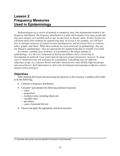
<strong>Lesson</strong> 2<br />
<strong>Frequency</strong> <strong>Measures</strong><br />
<strong>Used</strong> <strong>in</strong> Epidemiology<br />
Epidemiologists use a variety of methods to summarize data. One fundamental method is the<br />
frequency distribution. <strong>The</strong> frequency distribution is a table which displays how many people fall<br />
<strong>in</strong>to each category of a variable such as age, <strong>in</strong>come level, or disease status. In later lessons you<br />
will learn about other methods for summariz<strong>in</strong>g data. In <strong>Lesson</strong> 3, for example, you will learn<br />
how to calculate measures of central location and dispersion, and <strong>in</strong> <strong>Lesson</strong> 4 how to construct<br />
tables, graphs, and charts. While these methods are used extensively <strong>in</strong> epidemiology, they are<br />
not limited to epidemiology—they are appropriate for summariz<strong>in</strong>g data <strong>in</strong> virtually every field.<br />
In contrast, count<strong>in</strong>g cases of disease <strong>in</strong> a population is the unique doma<strong>in</strong> of<br />
epidemiology—it is the core component of disease surveillance and a critical step <strong>in</strong><br />
<strong>in</strong>vestigat<strong>in</strong>g an outbreak. Case counts must be placed <strong>in</strong> proper perspective, however, by us<strong>in</strong>g<br />
rates to characterize the risk of disease for a population. Calculat<strong>in</strong>g rates for different<br />
subgroups of age, sex, exposure history and other characteristics may identify high-risk groups<br />
and causal factors. Such <strong>in</strong>formation is vital to the development and target<strong>in</strong>g of effective control<br />
and prevention measures.<br />
Objectives<br />
After study<strong>in</strong>g this lesson and answer<strong>in</strong>g the questions <strong>in</strong> the exercises, a student will be able<br />
to do the follow<strong>in</strong>g:<br />
• Construct a frequency distribution<br />
• Calculate* and <strong>in</strong>terpret the follow<strong>in</strong>g statistical measures:<br />
— ratios<br />
— proportions<br />
— <strong>in</strong>cidence rates, <strong>in</strong>clud<strong>in</strong>g attack rate<br />
— mortality rates<br />
— prevalence<br />
— years of potential life lost<br />
• Choose and apply the appropriate statistical measures<br />
* A calculator with square root and logarithmic functions is recommended.<br />
73
Page 74<br />
Pr<strong>in</strong>ciples of Epidemiology<br />
Introduction to<br />
<strong>Frequency</strong> Distributions<br />
Epidemiologic data come <strong>in</strong> many forms and sizes. One of the most common forms is a<br />
rectangular database made up of rows and columns. Each row conta<strong>in</strong>s <strong>in</strong>formation about one<br />
<strong>in</strong>dividual; each row is called a “record” or “observation.” Each column conta<strong>in</strong>s <strong>in</strong>formation<br />
about one characteristic such as race or date of birth; each column is called a “variable.” <strong>The</strong> first<br />
column of an epidemiologic database usually conta<strong>in</strong>s the <strong>in</strong>dividual’s name, <strong>in</strong>itials, or<br />
identification number which allows us to identify who is who.<br />
<strong>The</strong> size of the database depends on the number of records and the number of variables. A<br />
small database may fit on a s<strong>in</strong>gle sheet of paper; larger databases with thousands of records and<br />
hundreds of variables are best handled with a computer. When we <strong>in</strong>vestigate an outbreak, we<br />
usually create a database called a “l<strong>in</strong>e list<strong>in</strong>g.” In a l<strong>in</strong>e list<strong>in</strong>g, each row represents a case of the<br />
disease we are <strong>in</strong>vestigat<strong>in</strong>g. Columns conta<strong>in</strong> identify<strong>in</strong>g <strong>in</strong>formation, cl<strong>in</strong>ical details,<br />
descriptive epidemiology factors, and possible etiolgic factors.<br />
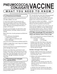
Look at the data <strong>in</strong> Table 2.1. How many of the cases are male When a database conta<strong>in</strong>s<br />
only a few records, we can easily pick out the <strong>in</strong>formation we need directly from the raw data.<br />
By scann<strong>in</strong>g the second column, we can see that five of the cases are male.<br />
ID<br />
Sex<br />
Table 2.1<br />
Neonatal listeriosis, General Hospital A, Costa Rica, 1989<br />
Culture<br />
Date<br />
Symptom<br />
Date<br />
DOB<br />
Delivery<br />
Type<br />
Delivery<br />
Site<br />
Outcome<br />
Admitt<strong>in</strong>g<br />
Symptoms<br />
CS F 6/2 6/2 6/2 vag<strong>in</strong>al Del rm Lived dyspnea<br />
CT M 6/8 6/2 6/2 c-section Oper rm Lived fever<br />
WG F 6/15 6/15 6/8 vag<strong>in</strong>al Emer rm Died dyspnea<br />
PA F 6/15 6/12 6/8 vag<strong>in</strong>al Del rm Lived fever<br />
SA F 6/15 6/15 6/11 c-section Oper rm Lived pneumonia<br />
HP F 6/22 6/20 6/14 c-section Oper rm Lived fever<br />
SS M 6/22 6/21 6/14 vag<strong>in</strong>al Del rm Lived fever<br />
JB F 6/22 6/18 6/15 c-section Oper rm Lived fever<br />
BS M 6/22 6/20 6/15 c-section Oper rm Lived pneumonia<br />
JG M 6/23 6/19 6/16 forceps Del rm Lived fever<br />
NC M 7/21 7/21 7/21 vag<strong>in</strong>al Del rm Died dyspnea<br />
Source: 11<br />
Abbreviations<br />
vag<strong>in</strong>al = vag<strong>in</strong>al delivery<br />
Del rm = delivery room<br />
Oper rm = operat<strong>in</strong>g room<br />
Emer rm = emergency room
<strong>Lesson</strong> 2: <strong>Frequency</strong> <strong>Measures</strong> <strong>Used</strong> <strong>in</strong> Epidemiology Page 75<br />
With larger databases, it becomes more difficult to pick out the <strong>in</strong>formation we want at a<br />
glance. Instead, we usually f<strong>in</strong>d it convenient to summarize variables <strong>in</strong>to tables called<br />
“frequency distributions.”<br />
A frequency distribution shows the values a variable can take, and the number of people or<br />
records with each value. For example, suppose we are study<strong>in</strong>g a group of women with ovarian<br />
cancer and have data on the parity of each woman—that is, the number of children each woman<br />
has given birth to. To construct a frequency distribution show<strong>in</strong>g these data, we first list, from<br />
the lowest observed value to the highest, all the values that the variable parity can take. For each<br />
parity value, we then enter the number of women who had given birth to that number of children.<br />
Table 2.2 shows what the result<strong>in</strong>g frequency distribution would look like. Notice that we listed<br />
all values of parity between the lowest and highest observed, even though there were no cases<br />
for some values. Notice also that each column is properly labeled, and that the total is given <strong>in</strong><br />
the bottom row.<br />
Source: 4<br />
Table 2.2<br />
Distribution of cases by parity, Ovarian Cancer Study,<br />
Centers for Disease Control, December 1980-September 1981<br />
Parity<br />
Number of Cases<br />
0 45<br />
1 25<br />
2 43<br />
3 32<br />
4 22<br />
5 8<br />
6 2<br />
7 0<br />
8 1<br />
9 0<br />
10 1<br />
Total 179
Page 76<br />
Pr<strong>in</strong>ciples of Epidemiology<br />
Exercise 2.1<br />
Listed below are data on parity collected from 19 women who participated <strong>in</strong> a study on<br />
reproductive health. Organize these data <strong>in</strong>to a frequency distribution.<br />
0, 2, 0, 0, 1, 3, 1, 4, 1, 8, 2, 2, 0, 1, 3, 5, 1, 7, 2<br />
Answers on page 127.<br />
Summariz<strong>in</strong>g Different Types of Variables<br />
Sometimes the values a variable can take are po<strong>in</strong>ts along a numerical scale, as <strong>in</strong> Table 2.2;<br />
sometimes they are categories, as <strong>in</strong> Table 2.3. When po<strong>in</strong>ts on a numerical scale are used, the<br />
scale is called an ord<strong>in</strong>al scale, because the values are ranked <strong>in</strong> a graded order. When<br />
categories are used, the measurement scale is called a nom<strong>in</strong>al scale, because it names the<br />
classes or categories of the variable be<strong>in</strong>g studied. In epidemiology, we often encounter nom<strong>in</strong>al<br />
variables with only two categories: alive or dead, ill or well, did or did not eat the potato salad.<br />
Table 2.3 shows a frequency distribution for a variable with only two possible values.<br />
Table 2.3<br />
Influenza vacc<strong>in</strong>ation status among residents of Nurs<strong>in</strong>g Home A<br />
Vacc<strong>in</strong>ated<br />
Number<br />
Yes 76<br />
No 125<br />
Total 201<br />
As you can see <strong>in</strong> Tables 2.2 and 2.3, both nom<strong>in</strong>al and ord<strong>in</strong>al scale data can be summarized<br />
<strong>in</strong> frequency distributions. Nom<strong>in</strong>al scale data are usually further summarized as ratios,<br />
proportions, and rates, which are described later <strong>in</strong> this lesson. Ord<strong>in</strong>al scale data are usually<br />
further summarized with measures of central location and measures of dispersion, which are<br />
described <strong>in</strong> <strong>Lesson</strong> 3.
<strong>Lesson</strong> 2: <strong>Frequency</strong> <strong>Measures</strong> <strong>Used</strong> <strong>in</strong> Epidemiology Page 77<br />
Introduction to<br />
<strong>Frequency</strong> <strong>Measures</strong><br />
In epidemiology, many nom<strong>in</strong>al variables have only two possible categories: alive or dead;<br />
case or control; exposed or unexposed; and so forth. Such variables are called dichotomous<br />
variables. <strong>The</strong> frequency measures we use with dichotomous variables are ratios, proportions,<br />
and rates.<br />
Before you learn about specific measures, it is important to understand the relationship<br />
between the three types of measures and how they differ from each other. All three measures are<br />
based on the same formula:<br />
Ratio, proportion, rate = y<br />
x × 10<br />
n<br />
In this formula, x and y are the two quantities that are be<strong>in</strong>g compared. <strong>The</strong> formula shows<br />
that x is divided by y. 10 n is a constant that we use to transform the result of the division <strong>in</strong>to a<br />
uniform quantity. 10 n is read as “10 to the nth power.” <strong>The</strong> size of 10 n may equal 1, 10, 100,<br />
1000 and so on depend<strong>in</strong>g upon the value of n. For example,<br />
10 0 = 1<br />
10 1 = 10<br />
10 2 = 10 × 10 = 100<br />
10 3 = 10 × 10 × 10 = 1000<br />
You will learn what value of 10 n to use when you learn about specific ratios, proportions, and<br />
rates.<br />
Ratios, Proportions, and Rates Compared<br />
In a ratio, the values of x and y may be completely <strong>in</strong>dependent, or x may be <strong>in</strong>cluded <strong>in</strong> y.<br />
For example, the sex of children attend<strong>in</strong>g an immunization cl<strong>in</strong>ic could be compared <strong>in</strong> either of<br />
the follow<strong>in</strong>g ways:<br />
(1)<br />
female<br />
male<br />
(2)<br />
female<br />
all<br />
In the first option, x (female) is completely <strong>in</strong>dependent of y (male). In the second, x (female)<br />
is <strong>in</strong>cluded <strong>in</strong> y (all). Both examples are ratios.<br />
A proportion, the second type of frequency measure used with dichotomous variables, is a<br />
ratio <strong>in</strong> which x is <strong>in</strong>cluded <strong>in</strong> y. Of the two ratios shown above, the first is not a proportion,<br />
because x is not a part of y. <strong>The</strong> second is a proportion, because x is part of y.<br />
<strong>The</strong> third type of frequency measure used with dichotomous variables, rate, is often a<br />
proportion, with an added dimension: it measures the occurrence of an event <strong>in</strong> a population over<br />
time. <strong>The</strong> basic formula for a rate is as follows:<br />
Rate =<br />
number of cases or events occurr<strong>in</strong>g dur<strong>in</strong>g a given time period<br />
population at risk dur<strong>in</strong>g the same time period<br />
× 10 n
Page 78<br />
Pr<strong>in</strong>ciples of Epidemiology<br />
Notice three important aspects of this formula.<br />
• <strong>The</strong> persons <strong>in</strong> the denom<strong>in</strong>ator must reflect the population from which the cases <strong>in</strong> the<br />
numerator arose.<br />
• <strong>The</strong> counts <strong>in</strong> the numerator and denom<strong>in</strong>ator should cover the same time period.<br />
• In theory, the persons <strong>in</strong> the denom<strong>in</strong>ator must be “at risk” for the event, that is, it should<br />
have been possible for them to experience the event.<br />
Example<br />
Dur<strong>in</strong>g the first 9 months of national surveillance for eos<strong>in</strong>ophilia-myalgia syndrome (EMS),<br />
CDC received 1,068 case reports which specified sex; 893 cases were <strong>in</strong> females, 175 <strong>in</strong> males.<br />
We will demonstrate how to calculate the female-to-male ratio for EMS (12).<br />
1. Def<strong>in</strong>e x and y: x = cases <strong>in</strong> females<br />
y = cases <strong>in</strong> males<br />
2. Identify x and y: x = 893<br />
y = 175<br />
3. Set up the ratio x/y: 893/175<br />
4. Reduce the fraction so that either<br />
x or y equals 1: 893/175 = 5.1 to 1<br />
Thus, there were just over 5 female EMS patients for each male EMS patient reported to<br />
CDC.<br />
Example<br />
Based on the data <strong>in</strong> the example above, we will demonstrate how to calculate the proportion<br />
of EMS cases that are male.<br />
1. Def<strong>in</strong>e x and y: x = cases <strong>in</strong> males<br />
y = all cases<br />
2. Identify x and y: x = 175<br />
y = 1,068<br />
3. Set up the ratio x/y: 175/1,068<br />
4. Reduce the fraction so that either<br />
x or y equals 1: 175/1,068 = 0.16/1 = 1/6.10<br />
Thus, about one out of every 6 reported EMS cases were <strong>in</strong> males.<br />
In the first example, we calculated the female-to-male ratio. In the second, we calculated the<br />
proportion of cases that were male. Is the female-to-male ratio a proportion<br />
<strong>The</strong> female-to-male ratio is not a proportion, s<strong>in</strong>ce the numerator (females) is not <strong>in</strong>cluded <strong>in</strong><br />
the denom<strong>in</strong>ator (males), i.e., it is a ratio, but not a proportion.
<strong>Lesson</strong> 2: <strong>Frequency</strong> <strong>Measures</strong> <strong>Used</strong> <strong>in</strong> Epidemiology Page 79<br />
As you can see from the above discussion, ratios, proportions, and rates are not three<br />
dist<strong>in</strong>ctly different k<strong>in</strong>ds of frequency measures. <strong>The</strong>y are all ratios: proportions are a particular<br />
type ratio, and some rates are a particular type of proportion. In epidemiology, however, we<br />
often shorten the terms for these measures <strong>in</strong> a way that makes it sound as though they are<br />
completely different. When we call a measure a ratio, we usually mean a nonproportional ratio;<br />
when we call a measure a proportion, we usually mean a proportional ratio that doesn’t measure<br />
an event over time, and when we use the term rate, we frequently refer to a proportional ratio<br />
that does measure an event <strong>in</strong> a population over time.<br />
Uses of Ratios, Proportions, and Rates<br />
In public health, we use ratios and proportions to characterize populations by age, sex, race,<br />
exposures, and other variables. In the example of the EMS cases we characterized the population<br />
by sex. In Exercise 2.1 you will be asked to characterize a series of cases by selected variables.<br />
We also use ratios, proportions, and, most important rates to describe three aspects of the<br />
human condition: morbidity (disease), mortality (death) and natality (birth). Table 2.4 shows<br />
some of the specific ratios, proportions, and rates we use for each of these classes of events.<br />
Table 2.4<br />
<strong>Frequency</strong> of measures by type of event described<br />
Condition Ratios Proportions Rates<br />
Morbidity<br />
(Disease)<br />
Mortality<br />
(Death)<br />
Natality<br />
(Birth)<br />
Risk ratio<br />
(Relative risk)<br />
Rate ratio<br />
Odds ratio<br />
Death-to-case ratio<br />
Maternal mortality rate<br />
Proportionate mortality<br />
ratio<br />
Postneonatal mortality<br />
rate<br />
Attributable<br />
proportion<br />
Po<strong>in</strong>t prevalence<br />
Proportionate<br />
mortality<br />
Case-fatality rate<br />
Low birth<br />
weight ratio<br />
Incidence rate<br />
Attack rate<br />
Secondary attack rate<br />
Person-time rate<br />
Period prevalence<br />
Crude mortality rate<br />
Cause-specific mortality<br />
rate<br />
Age-specific mortality rate<br />
Sex-specific mortality rate<br />
Race-specific mortality rate<br />
Age-adjusted mortality rate<br />
Neonatal mortality rate<br />
Infant mortality rate<br />
Years of potential life lost<br />
rate<br />
Crude birth rate<br />
Crude fertility rate<br />
Crude rate of natural<br />
<strong>in</strong>crease
Page 80<br />
Pr<strong>in</strong>ciples of Epidemiology<br />
Exercise 2.2<br />
<strong>The</strong> l<strong>in</strong>e list<strong>in</strong>g <strong>in</strong> Table 2.1, page 74, presents some of the <strong>in</strong>formation collected on <strong>in</strong>fants born<br />
at General Hospital A with neonatal listeriosis.<br />
a. What is the ratio of males to females<br />
b. What proportion of <strong>in</strong>fants lived<br />
c. What proportion of <strong>in</strong>fants were delivered <strong>in</strong> a delivery room<br />
d. What is the ratio of operat<strong>in</strong>g room deliveries to delivery room deliveries<br />
Answers on page 127.
<strong>Lesson</strong> 2: <strong>Frequency</strong> <strong>Measures</strong> <strong>Used</strong> <strong>in</strong> Epidemiology Page 81<br />
Morbidity <strong>Frequency</strong> <strong>Measures</strong><br />
To describe the presence of disease <strong>in</strong> a population, or the probability (risk) of its occurrence,<br />
we use one of the morbidity frequency measures. In public health terms, disease <strong>in</strong>cludes illness,<br />
<strong>in</strong>jury, or disability. Table 2.4 shows several morbidity measures. All of these can be further<br />
elaborated <strong>in</strong>to specific measures for age, race, sex, or some other characteristic of a particular<br />
population be<strong>in</strong>g described. We will describe how you calculate each of the morbidity measures<br />
and when you would use it. Table 2.5 shows a summary of the formulas for frequently used<br />
morbidity measures.<br />
Table 2.5<br />
Frequently used measures of morbidity<br />
Measure Numerator (x) Denom<strong>in</strong>ator (y)<br />
Incidence Rate # new cases of a specified average population<br />
disease reported dur<strong>in</strong>g a dur<strong>in</strong>g time <strong>in</strong>terval<br />
given time <strong>in</strong>terval<br />
Expressed per<br />
Number at Risk(10 n )<br />
varies:<br />
10 n where<br />
n = 2,3,4,5,6<br />
Attack Rate<br />
# new cases of a specified<br />
disease reported dur<strong>in</strong>g an<br />
epidemic period<br />
population at start of<br />
the epidemic period<br />
varies<br />
10 n where<br />
n = 2,3,4,5,6<br />
Secondary<br />
Attack Rate<br />
# new cases of a specified<br />
disease among contacts of<br />
known cases<br />
size of contract<br />
population at risk<br />
varies:<br />
10 n where<br />
n = 2,3,4,5,6<br />
Po<strong>in</strong>t<br />
Prevalence<br />
# current cases, new and<br />
old, of a specified disease<br />
at a given po<strong>in</strong>t <strong>in</strong> time<br />
estimated population<br />
at the same po<strong>in</strong>t <strong>in</strong><br />
time<br />
varies:<br />
10 n where<br />
n = 2,3,4,5,6<br />
Period<br />
Prevalence<br />
# current cases, new and<br />
old, of a specified disease<br />
identified over a given time<br />
<strong>in</strong>terval<br />
estimated population<br />
at mid-<strong>in</strong>terval<br />
varies:<br />
10 n where<br />
n = 2,3,4,5,6<br />
Incidence Rates<br />
Incidence rates are the most common way of measur<strong>in</strong>g and compar<strong>in</strong>g the frequency of<br />
disease <strong>in</strong> populations. We use <strong>in</strong>cidence rates <strong>in</strong>stead of raw numbers for compar<strong>in</strong>g disease<br />
occurrence <strong>in</strong> different populations because rates adjust for differences <strong>in</strong> population sizes. <strong>The</strong><br />
<strong>in</strong>cidence rate expresses the probability or risk of illness <strong>in</strong> a population over a period of time.<br />
S<strong>in</strong>ce <strong>in</strong>cidence is a measure of risk, when one population has a higher <strong>in</strong>cidence of disease<br />
than another, we say that the first population is at a higher risk of develop<strong>in</strong>g disease than the<br />
second, all other factors be<strong>in</strong>g equal. We can also express this by say<strong>in</strong>g that the first population<br />
is a high-risk group relative to the second population.
Page 82<br />
Pr<strong>in</strong>ciples of Epidemiology<br />
An <strong>in</strong>cidence rate (sometimes referred to simply as <strong>in</strong>cidence) is a measure of the frequency<br />
with which an event, such as a new case of illness, occurs <strong>in</strong> a population over a period of time.<br />
<strong>The</strong> formula for calculat<strong>in</strong>g an <strong>in</strong>cidence rate follows:<br />
Incidence rate =<br />
new cases ocurr<strong>in</strong>g dur<strong>in</strong>g a given time period<br />
population at risk dur<strong>in</strong>g the same time period<br />
× 10 n<br />
Example<br />
In 1989, 733,151 new cases of gonorrhea were reported among the United States civilian<br />
population (2). <strong>The</strong> 1989 mid-year U.S. civilian population was estimated to be 246,552,000. For<br />
these data we will use a value of 10 5 for 10 n . We will calculate the 1989 gonorrhea <strong>in</strong>cidence rate<br />
for the U.S. civilian population us<strong>in</strong>g these data.<br />
1. Def<strong>in</strong>e x and y: x = new cases of gonorrhea <strong>in</strong> U.S. civilians dur<strong>in</strong>g 1989<br />
y = U.S. civilian population <strong>in</strong> 1989<br />
2. Identify x, y, and 10 n : x = 733,151<br />
y = 246,552,000<br />
10 n = 10 5 = 100,000<br />
3. Calculate (x/y) × 10 n :<br />
733,151<br />
× 10 5 = .002974 × 100,000 = 297.4 per 100,000<br />
246,552,000<br />
or approximately 3 reported cases per 1,000 population <strong>in</strong> 1989.<br />
<strong>The</strong> numerator of an <strong>in</strong>cidence rate should reflect new cases of disease which occurred or<br />
were diagnosed dur<strong>in</strong>g the specified period. <strong>The</strong> numerator should not <strong>in</strong>clude cases which<br />
occurred or were diagnosed earlier.<br />
Notice that the denom<strong>in</strong>ator is the population at risk. This means that persons who are<br />
<strong>in</strong>cluded <strong>in</strong> the denom<strong>in</strong>ator should be able to develop the disease that is be<strong>in</strong>g described dur<strong>in</strong>g<br />
the time period covered. Unfortunately, unless we conduct a special study, we usually cannot<br />
identify and elim<strong>in</strong>ate persons who are not susceptible to the disease from available population<br />
data. In practice, we usually use U.S. Census population counts or estimates for the midpo<strong>in</strong>t of<br />
the time period under consideration. If the population be<strong>in</strong>g studied is small and very specific,<br />
however—such as a nurs<strong>in</strong>g home population—we can and should use exact denom<strong>in</strong>ator data.<br />
<strong>The</strong> denom<strong>in</strong>ator should represent the population from which the cases <strong>in</strong> the numerator<br />
arose. For surveillance purposes, the population is usually def<strong>in</strong>ed geopolitically (e.g., United<br />
States; state of Georgia). <strong>The</strong> population, however, may be def<strong>in</strong>ed by affiliation or membership<br />
(e.g., employee of Company X), common experience (underwent childhood thyroid irradiation),<br />
or any other characteristic which def<strong>in</strong>es a population appropriate for the cases <strong>in</strong> the numerator.<br />
Notice <strong>in</strong> the example above that the numerator was limited to civilian cases. <strong>The</strong>refore, it was<br />
necessary for us to restrict the denom<strong>in</strong>ator to civilians as well.
<strong>Lesson</strong> 2: <strong>Frequency</strong> <strong>Measures</strong> <strong>Used</strong> <strong>in</strong> Epidemiology Page 83<br />
Depend<strong>in</strong>g on the circumstances, the most appropriate denom<strong>in</strong>ator will be one of the<br />
follow<strong>in</strong>g:<br />
• average size of the population over the time period<br />
• size of the population (either total or at risk) at the middle of the time period<br />
• size of the population at the start of the time period<br />
For 10 n , any value of n can be used. For most nationally notifiable diseases, a value of<br />
100,000 or 10 5 is used for 10 n . In the example above, 10 5 is used s<strong>in</strong>ce gonorrhea is a nationally<br />
notifiable disease. Otherwise, we usually select a value for 10 n so that the smallest rate calculated<br />
<strong>in</strong> a series yields a small whole number (for example, 4.2/100, not 0.42/1,000; 9.6/100,000, not<br />
0.96/1,000,000).<br />
S<strong>in</strong>ce any value of n is possible, the <strong>in</strong>vestigator should clearly <strong>in</strong>dicate which value is be<strong>in</strong>g<br />
used. In our example above we selected a value of 100,000; therefore, our <strong>in</strong>cidence rate is<br />
reported as “297.4 per 100,000.” In a table where a 10 n value is used, the <strong>in</strong>vestigator could<br />
either specify “Rate per 1,000” at the head of the column <strong>in</strong> which rates are presented, or specify<br />
“/1,000” beside each rate shown.<br />
Rates imply a change over time. For disease <strong>in</strong>cidence rates, the change is from a healthy<br />
state to disease. <strong>The</strong> period of time must be specified. For surveillance purposes, the period of<br />
time most commonly used is the calendar year, but any <strong>in</strong>terval may be used as long as the limits<br />
of the <strong>in</strong>terval are identified.<br />
When the denom<strong>in</strong>ator is the size of the population at the start of the time period, the<br />
measure is sometimes called cumulative <strong>in</strong>cidence. This measure is a proportion, because all<br />
persons <strong>in</strong> the numerator are also <strong>in</strong> the denom<strong>in</strong>ator. It is a measure of the probability or risk<br />
of disease, i.e., what proportion of the population will develop illness dur<strong>in</strong>g the specified time<br />
period. In contrast, the <strong>in</strong>cidence rate is like velocity or speed measured <strong>in</strong> miles per hour. It<br />
<strong>in</strong>dicates how quickly people become ill measured <strong>in</strong> people per year.<br />
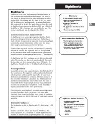
Example<br />
Figure 2.1 represents ten episodes of an illness <strong>in</strong> a population of 20 over a period of 16<br />
months. Each horizontal l<strong>in</strong>e represents the portion of time one person spends be<strong>in</strong>g ill. <strong>The</strong> l<strong>in</strong>e<br />
beg<strong>in</strong>s on the date of onset and ends on the date of death or on the date of recovery.<br />
In this example we will calculate the <strong>in</strong>cidence rate from October 1, 1990 to September 30,<br />
1990, us<strong>in</strong>g the midpo<strong>in</strong>t population as the denom<strong>in</strong>ator.<br />
Note that the total population is 20. We will use 10 n = 100.<br />
Incidence rate, October 1, 1990 to September 30, 1991; for the denom<strong>in</strong>ator use the total<br />
population at midpo<strong>in</strong>t (total population m<strong>in</strong>us those who have died before April 1, 1991).
Page 84<br />
Pr<strong>in</strong>ciples of Epidemiology<br />
Figure 2.1<br />
Ten episodes of an illness <strong>in</strong> a population of 20<br />
Date of onset of illness<br />
Person #<br />
1<br />
2<br />
3<br />
4<br />
5<br />
6<br />
7<br />
8<br />
9<br />
10<br />
Date of death<br />
Date of recovery<br />
Oct. 1, 1990 Apr. 1, 1991 Sep. 30, 1991<br />
x = new cases occurr<strong>in</strong>g 10/1/90−9/30/91 = 4<br />
y = total population at midpo<strong>in</strong>t = 20 − 2 = 18<br />
x × 10 n 4 22<br />
= × 100 =<br />
y 18 100<br />
So the one-year <strong>in</strong>cidence was 22 cases per 100 population.
<strong>Lesson</strong> 2: <strong>Frequency</strong> <strong>Measures</strong> <strong>Used</strong> <strong>in</strong> Epidemiology Page 85<br />
Exercise 2.3<br />
In 1990, 41,595 new cases of AIDS were reported <strong>in</strong> the United States (3). <strong>The</strong> 1990 midyear<br />
population was estimated to be 248,710,000. Calculate the 1990 AIDS <strong>in</strong>cidence rate. (Note: To<br />
facilitate computation with a calculator, both numerator and denom<strong>in</strong>ator could first be divided<br />
by 1,000.)<br />
Answer on page 128.<br />
Prevalence<br />
Prevalence, sometimes referred to as prevalence rate, is the proportion of persons <strong>in</strong> a<br />
population who have a particular disease or attribute at a specified po<strong>in</strong>t <strong>in</strong> time or over a<br />
specified period of time. <strong>The</strong> formula for presence of disease is:<br />
Prevalence =<br />
all new and pre - exist<strong>in</strong>g cases dur<strong>in</strong>g a given time period<br />
population dur<strong>in</strong>g the same time period<br />
× 10 n<br />
<strong>The</strong> formula for prevalence of an attribute is:<br />
Prevalence =<br />
persons hav<strong>in</strong>g a particular attribute dur<strong>in</strong>g a given time period<br />
population dur<strong>in</strong>g the same time period<br />
× 10 n<br />
<strong>The</strong> value of 10 n is usually 1 or 100 for common attributes. <strong>The</strong> value of 10 n may be 1,000,<br />
100,000, or even 1,000,000 for rare traits and for most diseases.
Page 86<br />
Pr<strong>in</strong>ciples of Epidemiology<br />
Po<strong>in</strong>t vs. period prevalence<br />
<strong>The</strong> amount of disease present <strong>in</strong> a population is constantly chang<strong>in</strong>g. Sometimes, we want to<br />
know how much of a particular disease is present <strong>in</strong> a population at a s<strong>in</strong>gle po<strong>in</strong>t <strong>in</strong> time—to get<br />
a k<strong>in</strong>d of “stop action” or “snapshot” look at the population with regard to that disease. We use<br />
po<strong>in</strong>t prevalence for that purpose. <strong>The</strong> numerator <strong>in</strong> po<strong>in</strong>t prevalence is the number of persons<br />
with a particular disease or attribute on a particular date. Po<strong>in</strong>t prevalence is not an <strong>in</strong>cidence<br />
rate, because the numerator <strong>in</strong>cludes pre-exist<strong>in</strong>g cases; it is a proportion, because the persons <strong>in</strong><br />
the numerator are also <strong>in</strong> the denom<strong>in</strong>ator.<br />
At other times we want to know how much of a particular disease is present <strong>in</strong> a population<br />
over a longer period. <strong>The</strong>n, we use period prevalence. <strong>The</strong> numerator <strong>in</strong> period prevalence is the<br />
number of persons who had a particular disease or attribute at any time dur<strong>in</strong>g a particular<br />
<strong>in</strong>terval. <strong>The</strong> <strong>in</strong>terval can be a week, month, year, decade, or any other specified time period.<br />
Example<br />
In a survey of patients at a sexually transmitted disease cl<strong>in</strong>ic <strong>in</strong> San Francisco, 180 of 300<br />
patients <strong>in</strong>terviewed reported use of a condom at least once dur<strong>in</strong>g the 2 months before the<br />
<strong>in</strong>terview (1). <strong>The</strong> period prevalence of condom use <strong>in</strong> this population over the last 2 months is<br />
calculated as:<br />
1. Identify x and y: x = condom users = 180<br />
y = total = 300<br />
2. Calculate (x/y) × 10 n : 180/300 × 100 = 60.0%.<br />
Thus, the prevalence of condom use <strong>in</strong> the 2 months before the study was 60% <strong>in</strong> this<br />
population of patients.<br />
Comparison of prevalence and <strong>in</strong>cidence<br />
<strong>The</strong> prevalence and <strong>in</strong>cidence of disease are frequently confused. <strong>The</strong>y are similar, but differ<br />
<strong>in</strong> what cases are <strong>in</strong>cluded <strong>in</strong> the numerator.<br />
Numerator of Incidence = new cases occurr<strong>in</strong>g dur<strong>in</strong>g a given time period<br />
Numerator of Prevalence = all cases present dur<strong>in</strong>g a given time period<br />
As you can see, the numerator of an <strong>in</strong>cidence rate consists only of persons whose illness<br />
began dur<strong>in</strong>g a specified <strong>in</strong>terval. <strong>The</strong> numerator for prevalence <strong>in</strong>cludes all persons ill from a<br />
specified cause dur<strong>in</strong>g a specified <strong>in</strong>terval (or at a specified po<strong>in</strong>t <strong>in</strong> time) regardless of when<br />
the illness began. It <strong>in</strong>cludes not only new cases, but also old cases represent<strong>in</strong>g persons who<br />
rema<strong>in</strong>ed ill dur<strong>in</strong>g some portion of the specified <strong>in</strong>terval. A case is counted <strong>in</strong> prevalence until<br />
death or recovery occurs.
<strong>Lesson</strong> 2: <strong>Frequency</strong> <strong>Measures</strong> <strong>Used</strong> <strong>in</strong> Epidemiology Page 87<br />
Example<br />
Two surveys were done of the same community 12 months apart. Of 5,000 people surveyed<br />
the first time, 25 had antibodies to histoplasmosis. Twelve months later, 35 had antibodies,<br />
<strong>in</strong>clud<strong>in</strong>g the orig<strong>in</strong>al 25. We will calculate the prevalence at the second survey, and compare the<br />
prevalence with the 1-year <strong>in</strong>cidence.<br />
1. Prevalence at the second survey:<br />
x = antibody positive at second survey = 35<br />
y = population = 5,000<br />
x/y × 10 n = 35/5,000 × 1,000 = 7 per 1,000<br />
2. Incidence dur<strong>in</strong>g the 12-month period:<br />
x = number of new positives dur<strong>in</strong>g the 12-month period = 35 − 25 = 10<br />
y = population at risk = 5,000 − 25 = 4,975<br />
x/y × 10 n = 10/4,975 × 1,000 = 2 per 1,000<br />
Prevalence is based on both <strong>in</strong>cidence (risk) and duration of disease. High prevalence of a<br />
disease with<strong>in</strong> a population may reflect high risk, or it may reflect prolonged survival without<br />
cure. Conversely, low prevalence may <strong>in</strong>dicate low <strong>in</strong>cidence, a rapidly fatal process, or rapid<br />
recovery.<br />
We often use prevalence rather than <strong>in</strong>cidence to measure the occurrence of chronic diseases<br />
such as osteoarthritis which have long duration and dates of onset which are difficult to p<strong>in</strong>po<strong>in</strong>t.
Page 88<br />
Pr<strong>in</strong>ciples of Epidemiology<br />
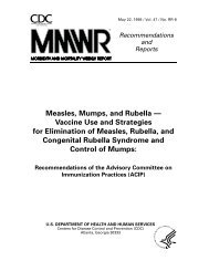
Exercise 2.4<br />
In the example on page 83 <strong>in</strong>cidence rates for the data shown <strong>in</strong> Figure 2.1 were calculated.<br />
Recall that Figure 2.1 represents ten episodes of an illness <strong>in</strong> a population of 20 over a period of<br />
16 months. Each horizontal l<strong>in</strong>e represents the portion of time one person spends be<strong>in</strong>g ill. <strong>The</strong><br />
l<strong>in</strong>e beg<strong>in</strong>s on the date of onset and ends on the date of death or recovery.<br />
Figure 2.1<br />
Ten episodes of an illness <strong>in</strong> a population of 20, revisited<br />
Date of onset of illness<br />
Person #<br />
1<br />
2<br />
3<br />
4<br />
5<br />
6<br />
7<br />
8<br />
9<br />
10<br />
Date of death<br />
Date of recovery<br />
Oct. 1, 1990 Apr. 1, 1991 Sep. 30, 1991<br />
Calculate the follow<strong>in</strong>g rates:<br />
a. Po<strong>in</strong>t prevalence on October 1, 1990<br />
b. Period prevalence, October 1, 1990 to September 30, 1991<br />
Answer on page 128.
<strong>Lesson</strong> 2: <strong>Frequency</strong> <strong>Measures</strong> <strong>Used</strong> <strong>in</strong> Epidemiology Page 89<br />
Attack Rate<br />
An attack rate is a variant of an <strong>in</strong>cidence rate, applied to a narrowly def<strong>in</strong>ed population<br />
observed for a limited time, such as dur<strong>in</strong>g an epidemic. <strong>The</strong> attack rate is usually expressed as a<br />
percent, so 10 n equals 100.<br />
For a def<strong>in</strong>ed population (the population at risk), dur<strong>in</strong>g a limited time period,<br />
Attack rate =<br />
Example<br />
Number of new cases among the<br />
Population at risk at the beg<strong>in</strong>n<strong>in</strong>g<br />
population dur<strong>in</strong>g the period<br />
of the period<br />
× 100<br />
Of 75 persons who attended a church picnic, 46 subsequently developed gastroenteritis. To<br />
calculate the attack rate of gastroenteritis we first def<strong>in</strong>e the numerator and denom<strong>in</strong>ator:<br />
x = Cases of gastroenteritis occurr<strong>in</strong>g with<strong>in</strong> the <strong>in</strong>cubation period for gastroenteritis among<br />
persons who attended the picnic = 46<br />
y = Number of persons at the picnic = 75<br />
46<br />
<strong>The</strong>n, the attack rate for gastroenteritis is × 100 = 61%<br />
75<br />
Notice that the attack rate is a proportion—the persons <strong>in</strong> the numerator are also <strong>in</strong> the<br />
denom<strong>in</strong>ator. This proportion is a measure of the probability or risk of becom<strong>in</strong>g a case. In the<br />
example above, we could say that, among persons who attended the picnic, the probability of<br />
develop<strong>in</strong>g gastroenteritis was 61%, or the risk of develop<strong>in</strong>g gastroenteritis was 61%.<br />
Secondary Attack Rate<br />
A secondary attack rate is a measure of the frequency of new cases of a disease among the<br />
contacts of known cases. <strong>The</strong> formula is as follows:<br />
Secondary attack rate =<br />
Number of cases among<br />
contacts<br />
of<br />
total number of<br />
primary cases dur<strong>in</strong>g the<br />
contacts<br />
period<br />
× 10 n<br />
To calculate the total number of household contacts, we usually subtract the number of<br />
primary cases from the total number of people resid<strong>in</strong>g <strong>in</strong> those households.<br />
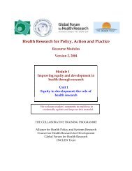
Example<br />
Seven cases of hepatitis A occurred among 70 children attend<strong>in</strong>g a child care center. Each<br />
<strong>in</strong>fected child came from a different family. <strong>The</strong> total number of persons <strong>in</strong> the 7 affected<br />
families was 32. One <strong>in</strong>cubation period later, 5 family members of the 7 <strong>in</strong>fected children also<br />
developed hepatitis A. We will calculate the attack rate <strong>in</strong> the child care center and the secondary<br />
attack rate among family contacts of those cases.<br />
1. Attack rate <strong>in</strong> child care center:<br />
x = cases of hepatitis A among children <strong>in</strong> child care center = 7<br />
y = number of children enrolled <strong>in</strong> the child care center = 70<br />
x 7<br />
Attack rate = × 100 = × 100 = 10%<br />
y 70
Page 90<br />
Pr<strong>in</strong>ciples of Epidemiology<br />
Figure 2.2<br />
Secondary spread from child care center to homes<br />
child attend<strong>in</strong>g child<br />
care center<br />
child with hepatitis A<br />
family member<br />
family member who<br />
developed hepatitis A<br />
CHILD CARE CENTER<br />
2. Secondary attack rate:<br />
x = cases of hepatitis A among family contacts of children with hepatitis<br />
A = 5<br />
y = number of persons at risk <strong>in</strong> the families (total number of family members—children<br />
already <strong>in</strong>fected) = 32 − 7 = 25<br />
x 5<br />
Secondary attack rate = × 100 = × 100 = 20%<br />
y 25
<strong>Lesson</strong> 2: <strong>Frequency</strong> <strong>Measures</strong> <strong>Used</strong> <strong>in</strong> Epidemiology Page 91<br />
Exercise 2.5<br />
In a particular community, 115 persons <strong>in</strong> a population of 4,399 became ill with a disease of<br />
unknown etiology. <strong>The</strong> 115 cases occurred <strong>in</strong> 77 households. <strong>The</strong> total number of persons liv<strong>in</strong>g<br />
<strong>in</strong> these 77 households was 424.<br />
a. Calculate the overall attack rate <strong>in</strong> the community.<br />
b. Calculate the secondary attack rate <strong>in</strong> the affected households, assum<strong>in</strong>g that only one case per<br />
household was a primary (community-acquired) case.<br />
c. Is the disease distributed evenly throughout the population<br />
Answer on page 128.
Page 92<br />
Pr<strong>in</strong>ciples of Epidemiology<br />
Person-time Rate<br />
A person-time rate is a type of <strong>in</strong>cidence rate that directly <strong>in</strong>corporates time <strong>in</strong>to the<br />
denom<strong>in</strong>ator. Typically, each person is observed from a set beg<strong>in</strong>n<strong>in</strong>g po<strong>in</strong>t to an established end<br />
po<strong>in</strong>t (onset of disease, death, migration out of the study, or end of the study). <strong>The</strong> numerator is<br />
still the number of new cases, but the denom<strong>in</strong>ator is a little different. <strong>The</strong> denom<strong>in</strong>ator is the<br />
sum of the time each person is observed, totaled for all persons.<br />
Person-time rate =<br />
Number of cases dur<strong>in</strong>g<br />
Time each person<br />
was observed,totaled<br />
observation period<br />
for all persons<br />
× 10 n<br />
For example, a person enrolled <strong>in</strong> a study who develops the disease of <strong>in</strong>terest 5 years later<br />
contributes 5 person-years to the denom<strong>in</strong>ator. A person who is disease-free at one year and who<br />
is then lost to follow-up contributes just that 1 person-year to the denom<strong>in</strong>ator. Person-time rates<br />
are often used <strong>in</strong> cohort (follow-up) studies of diseases with long <strong>in</strong>cubation or latency periods,<br />
such as some occupationally related diseases, AIDS, and chronic diseases.<br />
Example<br />
Investigators enrolled 2,100 men <strong>in</strong> a study and followed them over 4 years to determ<strong>in</strong>e the<br />
rate of heart disease. <strong>The</strong> follow-up data are provided below. We will calculate the person-time<br />
<strong>in</strong>cidence rate of disease. We assume that persons diagnosed with disease and those lost to<br />
follow-up were disease-free for half of the year, and thus contribute ½ year to the denom<strong>in</strong>ator.<br />
Initial enrollment: 2,100 men free of disease<br />
After 1 year: 2,000 disease-free, 0 with disease, 100 lost to follow-up<br />
After 2 years: 1,900 disease-free, 1 with disease, 99 lost to follow-up<br />
After 3 years: 1,100 disease-free, 7 with disease, 793 lost to follow-up<br />
After 4 years: 700 disease-free, 8 with disease, 392 lost to follow-up<br />
1. Identify x: x = cases diagnosed = 1 + 7 + 8 = 16<br />
2. Calculate y, the person-years of observation:<br />
1 1 1 1 1 1<br />
(2,000 + × 100) + (1,900 + × 1 + × 99) + (1,100 + × 7 + × 793) + (700 + × 8<br />
2 2 2 2 2 2<br />
+ 2<br />
1 × 392) = 6,400 person-years of observation.<br />
A second way to calculate the person-years of observation is to turn the data around to reflect<br />
how many people were followed for how many years, as follows:<br />
700 men × 4.0 years = 2,800 person-years<br />
8 + 392 = 400 men × 3.5 years = 1,400 person-years<br />
7 + 793 = 800 men × 2.5 years = 2,000 person-years<br />
1 + 99 = 100 men × 1.5 years = 150 person-years<br />
0 + 100 = 100 men × 0.5 years = 50 person-years<br />
Total = 6,400 person-years of observation
<strong>Lesson</strong> 2: <strong>Frequency</strong> <strong>Measures</strong> <strong>Used</strong> <strong>in</strong> Epidemiology Page 93<br />
This is exactly equal to the average population at risk (1,600) times duration of follow-up (4<br />
years).<br />
3. Person-time rate =<br />
number of cases dur<strong>in</strong>g<br />
time each person was observed,totaled<br />
16<br />
= × 10 n = .0025 × 10 n<br />
6,<br />
400<br />
4 - year study<br />
for all persons<br />
× 10 n<br />
or, if 10 n is set at 1,000, there were 2.5 cases per 1,000 person-years of<br />
observation. This quantity is also commonly expressed as 2.5 cases per<br />
1,000 persons per year.<br />
In contrast, the attack rate comes out to 16/2,100 = 7.6 cases/1,000 population dur<strong>in</strong>g the 4-<br />
year period. This averages out to 1.9 cases per 1,000 persons per year. <strong>The</strong> attack rate is less<br />
accurate because it ignores persons lost to follow-up.<br />
<strong>The</strong> attack rate is more useful when we are <strong>in</strong>terested <strong>in</strong> the proportion of a population who<br />
becomes ill over a brief period, particularly dur<strong>in</strong>g the course of an epidemic. <strong>The</strong> person-time<br />
rate is more useful when we are <strong>in</strong>terested <strong>in</strong> how quickly people develop illnesses, assum<strong>in</strong>g a<br />
constant rate over time.<br />
Risk Ratio<br />
A risk ratio, or relative risk, compares the risk of some health-related event such as disease<br />
or death <strong>in</strong> two groups. <strong>The</strong> two groups are typically differentiated by demographic factors such<br />
as sex (e.g., males versus females) or by exposure to a suspected risk factor (e.g., consumption of<br />
potato salad or not). Often, you will see the group of primary <strong>in</strong>terest labeled the “exposed”<br />
group, and the comparison group labeled the “unexposed” group. We place the group that we are<br />
primarily <strong>in</strong>terested <strong>in</strong> the numerator; we place the group we are compar<strong>in</strong>g them with <strong>in</strong> the<br />
denom<strong>in</strong>ator:<br />
Risk Ratio =<br />
risk for<br />
Risk<br />
group of primary <strong>in</strong>terest<br />
for comparison group<br />
× 1<br />
<strong>The</strong> values used for the numerator and denom<strong>in</strong>ator should be ones that take <strong>in</strong>to account the<br />
size of the populations the two groups are drawn from. For measures of disease, the <strong>in</strong>cidence<br />
rate or attack rate of the disease <strong>in</strong> each group may be used. Notice that a value of 1 is used for<br />
10 n .<br />
A risk ratio of 1.0 <strong>in</strong>dicates identical risk <strong>in</strong> the two groups. A risk ratio greater than 1.0<br />
<strong>in</strong>dicates an <strong>in</strong>creased risk for the numerator group, while a risk ratio less than 1.0 <strong>in</strong>dicates a<br />
decreased risk for the numerator group (perhaps show<strong>in</strong>g a protective effect of the factor among<br />
the “exposed” numerator group).<br />
Example<br />
Us<strong>in</strong>g data from one of the classic studies of pellagra by Goldberger, we will calculate the<br />
risk ratio of pellagra for females versus males. Pellagra is a disease caused by dietary deficiency<br />
of niac<strong>in</strong> and characterized by dermatitis, diarrhea, and dementia. Data from a comparative study<br />
such as this one can be summarized <strong>in</strong> a two-by-two table. <strong>The</strong> “two-by-two” refers to the two
Page 94<br />
Pr<strong>in</strong>ciples of Epidemiology<br />
variables (sex and illness status), each with two categories. <strong>The</strong>se tables will be discussed <strong>in</strong><br />
more detail <strong>in</strong> <strong>Lesson</strong> 4. Data from the pellagra study are shown <strong>in</strong> Table 2.6. <strong>The</strong> totals for<br />
females and males are also shown.<br />
Table 2.6<br />
Number of cases for pellagra by sex, South Carol<strong>in</strong>a, 1920’s<br />
Pellagra<br />
Yes No Total<br />
Female a = 46 b = 1,438 1,484<br />
Male c = 18 d = 1,401 1,419<br />
Source: 6<br />
To calculate the risk ratio of pellagra for females versus males, we must first calculate the<br />
risk of illness among females and among males.<br />
a<br />
Risk of illness among females =<br />
a + b<br />
46<br />
= 1 , 484<br />
= .031<br />
c<br />
Risk of illness among males =<br />
c + d<br />
18<br />
= 1 , 419<br />
= .013<br />
<strong>The</strong>refore, the risk of illness among females is .031 or 3.1% and the risk of illness among males<br />
is .013 or 1.3%. In calculat<strong>in</strong>g the risk ratio for females versus males, females are the group of<br />
primary <strong>in</strong>terest and males are the comparison group. <strong>The</strong> formula is:<br />
Risk ratio =<br />
3.<br />
1%<br />
1.<br />
3%<br />
= 2.4<br />
<strong>The</strong> risk of pellagra <strong>in</strong> females appears to be 2.4 times higher than the risk <strong>in</strong> males.<br />
Example<br />
In the same study, the risk of pellagra among mill workers was 0.9%. <strong>The</strong> risk among those<br />
who did not work <strong>in</strong> the mill was 4.4%. <strong>The</strong> relative risk of pellagra for mill workers versus nonmill<br />
workers is calculated as:<br />
Relative risk = risk ratio = 0.9%/4.4% = 0.2<br />
<strong>The</strong> risk of pellagra <strong>in</strong> mill workers appears to be only 0.2 or one-fifth of the risk <strong>in</strong> non-mill<br />
workers. In other words, work<strong>in</strong>g <strong>in</strong> the mill appears to protect aga<strong>in</strong>st develop<strong>in</strong>g pellagra.<br />
<strong>The</strong> relative risk is called a measure of association because it quantifies the relationship<br />
(association) between the so-called exposure (sex, mill employment) and disease (pellagra).
<strong>Lesson</strong> 2: <strong>Frequency</strong> <strong>Measures</strong> <strong>Used</strong> <strong>in</strong> Epidemiology Page 95<br />
Rate Ratio<br />
A rate ratio compares two groups <strong>in</strong> terms of <strong>in</strong>cidence rates, person-time rates, or mortality<br />
rates. Like the risk ratio, the two groups are typically differentiated by demographic factors or by<br />
exposure to a suspected causative agent. <strong>The</strong> rate for the group of primary <strong>in</strong>terest is divided by<br />
the rate for the comparison group.<br />
Rate ratio =<br />
rate for group of primary <strong>in</strong>terest<br />
rate for comparison group<br />
× 1<br />
<strong>The</strong> <strong>in</strong>terpretation of the value of a rate ratio is similar to that of the risk ratio.<br />
Example<br />
<strong>The</strong> rate ratio quantifies the relative <strong>in</strong>cidence of a particular health event <strong>in</strong> two specified<br />
populations (one exposed to a suspected causative agent, one unexposed) over a specified period.<br />
For example, the data <strong>in</strong> Table 2.7a provide death rates from lung cancer taken from the classic<br />
study on smok<strong>in</strong>g and cancer by Doll and Hill (5). Us<strong>in</strong>g these data we will calculate the rate<br />
ratio of smokers of 1-14 cigarettes per day to nonsmokers. <strong>The</strong> “exposed group” is the smokers<br />
of 1-14 cigarettes per day. <strong>The</strong> “unexposed group” is the smokers of 0 cigarettes per day.<br />
Table 2.7a<br />
Death rates and rate ratios from lung cancer by daily cigarette consumption,<br />
Doll and Hill physician follow-up study, 1951-1961<br />
Death rates<br />
Cigarettes per day per 1000 per year Rate ratio<br />
0 (Nonsmokers)<br />
1-14<br />
15-24<br />
25+<br />
0.07<br />
0.57<br />
1.39<br />
2.27<br />
—<br />
____________<br />
____________<br />
____________<br />
Source: 5<br />
Rate ratio = 0.57 / 0.07 = 8.1<br />
<strong>The</strong> rate of lung cancer among smokers of 1-14 cigarettes is 8.1 times higher than the rate of<br />
lung cancer <strong>in</strong> nonsmokers.
Page 96<br />
Pr<strong>in</strong>ciples of Epidemiology<br />
Exercise 2.6<br />
Us<strong>in</strong>g data <strong>in</strong> Table 2.7a, calculate the follow<strong>in</strong>g rate ratios. Enter the ratios <strong>in</strong> Table 2.7a.<br />
Discuss what the various rate ratios show about the risk for lung cancer among cigarette<br />
smokers.<br />
a. Smokers of 15-24 cigarettes per day compared with nonsmokers<br />
b. Smokers of 25+ cigarettes per day compared with nonsmokers<br />
Answer on page 129.<br />
Odds Ratio<br />
An odds ratio is another measure of association which quantifies the relationship between an<br />
exposure and health outcome from a comparative study. <strong>The</strong> odds ratio is calculated as:<br />
ad<br />
Odds ratio = bc<br />
a = number of persons with disease and with exposure of <strong>in</strong>terest<br />
b = number of persons without disease, but with exposure of <strong>in</strong>terest<br />
c = number of persons with disease, but without exposure of <strong>in</strong>terest<br />
d = number of persons without disease and without exposure of <strong>in</strong>terest<br />
a + c = total number of persons with disease (“cases”)<br />
b + d = total number of persons without disease (“controls”)<br />
Note that <strong>in</strong> the two-by-two table, Table 2.6 on page 94, the same letters (a, b, c, and d) are<br />
used to label the four cells <strong>in</strong> the table. <strong>The</strong> odds ratio is sometimes called the cross-product<br />
ratio, because the numerator is the product of cell a and cell d, while the denom<strong>in</strong>ator is the<br />
product of cell b and cell c. A l<strong>in</strong>e from cell a to cell d (for the numerator) and another from cell<br />
b to cell c (for the denom<strong>in</strong>ator) creates an x or cross on the two-by-two table.
<strong>Lesson</strong> 2: <strong>Frequency</strong> <strong>Measures</strong> <strong>Used</strong> <strong>in</strong> Epidemiology Page 97<br />
Example<br />
To quantify the relationship between pellagra and sex, the odds ratio is calculated as:<br />
Odds ratio =<br />
46 × 1,<br />
401<br />
1,<br />
438 × 18<br />
= 2.5<br />
Notice that the odds ratio of 2.5 is fairly close to the risk ratio of 2.4. That is one of the<br />
attractive features of the odds ratio: when the health outcome is uncommon, the odds ratio<br />
provides a good approximation of the relative risk. Another attractive feature is that we can<br />
calculate the odds ratio if we know the values <strong>in</strong> four cells <strong>in</strong> the two-by-two table; we do not<br />
need to know the size of the total exposed group and the total unexposed group. This feature is<br />
particularly relevant when we analyze data from a case-control study, which has a group of cases<br />
(distributed <strong>in</strong> cells a and c of the two-by-two table) and a group of non-cases or controls<br />
(distributed <strong>in</strong> cells b and d). <strong>The</strong> size of the control group is arbitrary and the true size of the<br />
population from which the cases came is usually not known, so we usually cannot calculate rates<br />
or a relative risk. Nonetheless, we can still calculate an odds ratio, and <strong>in</strong>terpret it as an<br />
approximation of the relative risk.<br />
Attributable Proportion<br />
<strong>The</strong> attributable proportion, also known as the attributable risk percent, is a measure of the<br />
public health impact of a causative factor. In calculat<strong>in</strong>g this measure, we assume that the<br />
occurrence of disease <strong>in</strong> a group not exposed to the factor under study represents the basel<strong>in</strong>e or<br />
expected risk for that disease; we will attribute any risk above that level <strong>in</strong> the exposed group to<br />
their exposure. Thus, the attributable proportion is the proportion of disease <strong>in</strong> an exposed group<br />
attributable to the exposure. It represents the expected reduction <strong>in</strong> disease if the exposure could<br />
be removed (or never existed).<br />
For two specified subpopulations, identified as exposed or unexposed to a suspected risk<br />
factor, with risk of a health event recorded over a specified period,<br />
Attributable Proportion =<br />
(risk<br />
for exposed<br />
group) −(risk<br />
risk for exposed group<br />
for unexposed<br />
group)<br />
× 100%<br />
Attributable proportion can be calculated for rates <strong>in</strong> the same way.
Page 98<br />
Pr<strong>in</strong>ciples of Epidemiology<br />
Example<br />
Us<strong>in</strong>g the data <strong>in</strong> Table 2.7b, we will calculate the attributable proportion for persons who<br />
smoked 1-14 cigarettes per day.<br />
Table 2.7b<br />
Death rates and rate ratios from lung cancer by daily cigarette consumption<br />
Doll and Hill physician follow-up study, 1951-1961<br />
Cigarettes per day<br />
Death Rates<br />
per 1,000 per Year<br />
Rate Ratio<br />
Attributable<br />
Proportion<br />
0 (Nonsmokers)<br />
1-14<br />
15-24<br />
25+<br />
0.07<br />
0.57<br />
1.39<br />
2.27<br />
—<br />
8.1<br />
19.9<br />
32.4<br />
____________<br />
____________<br />
____________<br />
____________<br />
Source: 5<br />
1. Identify exposed group rate: lung cancer death rate for smokers of 1-14 cigarettes per day =<br />
0.57 per 1,000 per year<br />
2. Identify unexposed group rate: lung cancer death rate for nonsmokers = 0.07 per 1,000 per<br />
year<br />
3. Calculate attributable proportion:<br />
=<br />
0. 57 − 0.<br />
07<br />
0.<br />
57<br />
× 100%<br />
= 0.877 × 100%<br />
= 87.7%<br />
Thus, assum<strong>in</strong>g our data are valid (for example, the groups are comparable <strong>in</strong> age and other<br />
risk factors), then about 88% of the lung cancer <strong>in</strong> smokers of 1-14 cigarettes per day may be<br />
attributable to their smok<strong>in</strong>g. Approximately 12% of the lung cancer cases <strong>in</strong> this group would<br />
have occurred anyway.
<strong>Lesson</strong> 2: <strong>Frequency</strong> <strong>Measures</strong> <strong>Used</strong> <strong>in</strong> Epidemiology Page 99<br />
Exercise 2.7<br />
Us<strong>in</strong>g the data <strong>in</strong> Table 2.7b, calculate the attributable proportions for the follow<strong>in</strong>g:<br />
a. smokers of 15-24 cigarettes per day<br />
b. smokers of 25+ cigarettes per day<br />
Table 2.7b, revisited<br />
Death rates and rate ratios from lung cancer by daily cigarette consumption<br />
Doll and Hill physician follow-up study, 1951-1961<br />
Cigarettes per Day<br />
Death Rates<br />
per 1,000 per Year<br />
Rate Ratio<br />
Attributable<br />
Proportion<br />
0 (Nonsmokers)<br />
1-14<br />
15-24<br />
25+<br />
0.07<br />
0.57<br />
1.39<br />
2.27<br />
—<br />
8.1<br />
19.9<br />
32.4<br />
___________<br />
87.7%<br />
___________<br />
___________<br />
Source: 5<br />
Answer on page 129.
Page 100<br />
Pr<strong>in</strong>ciples of Epidemiology<br />
Mortality <strong>Frequency</strong> <strong>Measures</strong><br />
Mortality Rates<br />
A mortality rate is a measure of the frequency of occurrence of death <strong>in</strong> a def<strong>in</strong>ed population<br />
dur<strong>in</strong>g a specified <strong>in</strong>terval. For a def<strong>in</strong>ed population, over a specified period of time,<br />
Mortality rate =<br />
deaths occurr<strong>in</strong>g dur<strong>in</strong>g a given time period<br />
size of the population among which the deaths occurred<br />
× 10 n<br />
When mortality rates are based on vital statistics (e.g., counts of death certificates), the<br />
denom<strong>in</strong>ator most commonly used is the size of the population at the middle of the time period.<br />
In the United States, values of 1,000 and 100,000 are both used for 10 n for most types of<br />
mortality rates. Table 2.8 summarizes the formulas of frequently used mortality measures.<br />
Table 2.8<br />
Frequently used measures of mortality<br />
Measure Numerator (x) Denom<strong>in</strong>ator (y)<br />
Crude Death Rate<br />
total number of deaths<br />
reported dur<strong>in</strong>g a given<br />
time <strong>in</strong>terval<br />
Estimated mid-<strong>in</strong>terval<br />
population<br />
Expressed per<br />
number at risk (10 n )<br />
1,000 or 100,000<br />
Cause-specific<br />
Death Rate<br />
# deaths assigned to a<br />
specific cause dur<strong>in</strong>g a<br />
given time <strong>in</strong>terval<br />
Estimated mid-<strong>in</strong>terval<br />
population<br />
100,000<br />
Proportional Mortality<br />
# deaths assigned to a<br />
specific cause dur<strong>in</strong>g a<br />
given time <strong>in</strong>terval<br />
Total number of<br />
deaths from all causes<br />
dur<strong>in</strong>g the same<br />
<strong>in</strong>terval<br />
100 or 1,000<br />
Death-to-Case Ratio<br />
# deaths assigned to a<br />
specific disease dur<strong>in</strong>g a<br />
given time <strong>in</strong>terval<br />
# new cases of that<br />
disease reported<br />
dur<strong>in</strong>g the same time<br />
<strong>in</strong>terval<br />
100<br />
Neonatal Mortality Rate<br />
# deaths under 28 days of<br />
age dur<strong>in</strong>g a given time<br />
<strong>in</strong>terval<br />
# live births dur<strong>in</strong>g the<br />
same time <strong>in</strong>terval<br />
1,000<br />
Postneonatal<br />
Mortality Rate<br />
# deaths from 28 days to,<br />
but not <strong>in</strong>clud<strong>in</strong>g, 1 year of<br />
age, dur<strong>in</strong>g a given time<br />
<strong>in</strong>terval<br />
# live births dur<strong>in</strong>g the<br />
same time <strong>in</strong>terval<br />
1,000<br />
Infant Mortality Rate<br />
# deaths under 1 year of<br />
age dur<strong>in</strong>g a given time<br />
<strong>in</strong>terval<br />
#l live births reported<br />
dur<strong>in</strong>g the same time<br />
<strong>in</strong>terval<br />
1,000<br />
Maternal Mortality Rate<br />
# deaths assigned to<br />
pregnancy-related causes<br />
dur<strong>in</strong>g a given time <strong>in</strong>terval<br />
# live births dur<strong>in</strong>g the<br />
same time <strong>in</strong>terval<br />
100,000
<strong>Lesson</strong> 2: <strong>Frequency</strong> <strong>Measures</strong> <strong>Used</strong> <strong>in</strong> Epidemiology Page 101<br />
Crude mortality rate (crude death rate)<br />
<strong>The</strong> crude mortality rate is the mortality rate from all causes of death for a population. For<br />
10 n , we use 1,000 or 100,000.<br />
Cause-specific mortality rate<br />
<strong>The</strong> cause-specific mortality rate is the mortality rate from a specified cause for a population.<br />
<strong>The</strong> numerator is the number of deaths attributed to a specific cause. <strong>The</strong> denom<strong>in</strong>ator rema<strong>in</strong>s<br />
the size of the population at the midpo<strong>in</strong>t of the time period. For 10 n , we use 100,000.<br />
Age-specific mortality rate<br />
An age-specific mortality rate is a mortality rate limited to a particular age group. <strong>The</strong><br />
numerator is the number of deaths <strong>in</strong> that age group; the denom<strong>in</strong>ator is the number of persons <strong>in</strong><br />
that age group <strong>in</strong> the population. Some specific types of age-specific mortality rates are neonatal,<br />
postneonatal, and <strong>in</strong>fant mortality rates.<br />
Infant mortality rate<br />
<strong>The</strong> <strong>in</strong>fant mortality rate is one of the most commonly used measures for compar<strong>in</strong>g health<br />
services among nations. <strong>The</strong> numerator is the number of deaths among children under 1 year of<br />
age reported dur<strong>in</strong>g a given time period, usually a calendar year. <strong>The</strong> denom<strong>in</strong>ator is the number<br />
of live births reported dur<strong>in</strong>g the same time period. <strong>The</strong> <strong>in</strong>fant mortality rate is usually expressed<br />
per 1,000 live births.<br />
Is the <strong>in</strong>fant mortality rate a proportion Technically, it is a ratio but not a proportion.<br />
Consider the U.S <strong>in</strong>fant mortality rate for 1988. In 1988, 38,910 <strong>in</strong>fants died and 3.9 million<br />
children were born, for an <strong>in</strong>fant mortality rate of 9.95 per 1,000 (7). Undoubtedly, some of these<br />
deaths occurred among children born <strong>in</strong> 1987, but the denom<strong>in</strong>ator <strong>in</strong>cludes only children born <strong>in</strong><br />
1988.<br />
Neonatal mortality rate<br />
<strong>The</strong> neonatal period is def<strong>in</strong>ed as the period from birth up to but not <strong>in</strong>clud<strong>in</strong>g 28 days. <strong>The</strong><br />
numerator of the neonatal mortality rate therefore is the number of deaths among children under<br />
28 days of age dur<strong>in</strong>g a given time period. <strong>The</strong> denom<strong>in</strong>ator of the neonatal mortality rate, like<br />
that of the <strong>in</strong>fant mortality rate, is the number of live births reported dur<strong>in</strong>g the same time period.<br />
<strong>The</strong> neonatal mortality rate is usually expressed per 1,000 live births. In 1988, the neonatal<br />
mortality rate <strong>in</strong> the United States was 6.3 per 1,000 live births (7).<br />
Postneonatal mortality rate<br />
<strong>The</strong> postneonatal period is def<strong>in</strong>ed as the period from 28 days of age up to but not <strong>in</strong>clud<strong>in</strong>g<br />
1 year of age. <strong>The</strong> numerator of the postneonatal mortality rate therefore is the number of deaths<br />
among children from 28 days up to but not <strong>in</strong>clud<strong>in</strong>g 1 year of age dur<strong>in</strong>g a given time period.<br />
<strong>The</strong> denom<strong>in</strong>ator is the number of live births reported dur<strong>in</strong>g the same time period. <strong>The</strong><br />
postneonatal mortality rate is usually expressed per 1,000 live births. In 1988, the postneonatal<br />
mortality rate <strong>in</strong> the United States was 3.6 per 1,000 live births (7).
Page 102<br />
Pr<strong>in</strong>ciples of Epidemiology<br />
Maternal mortality rate<br />
<strong>The</strong> maternal mortality rate is really a ratio used to measure mortality associated with<br />
pregnancy. <strong>The</strong> numerator is the number of deaths assigned to causes related to pregnancy<br />
dur<strong>in</strong>g a given time period. <strong>The</strong> denom<strong>in</strong>ator is the number of live births reported dur<strong>in</strong>g the<br />
same time period. Because maternal mortality is much less common than <strong>in</strong>fant mortality, the<br />
maternal mortality rate is usually expressed per 100,000 live births. In 1988, the maternal<br />
mortality rate was 8.4 per 100,000 live births (7).<br />
Sex-specific mortality rate<br />
A sex-specific mortality rate is a mortality rate among either males or females. Both<br />
numerator and denom<strong>in</strong>ator are limited to the one sex.<br />
Race-specific mortality rate<br />
A race-specific mortality rate is a mortality rate limited to a specified racial group. Both<br />
numerator and denom<strong>in</strong>ator are limited to the specified race.<br />
Comb<strong>in</strong>ations of specific mortality rates<br />
Mortality rates can be further ref<strong>in</strong>ed to comb<strong>in</strong>ations that are cause-specific, age-specific,<br />
sex-specific, and/or race-specific. For example, the mortality rate attributed to HIV among 25- to<br />
44-year-olds <strong>in</strong> the United States <strong>in</strong> 1987 was 9,820 deaths among 77.6 million 25- to 44-yearolds,<br />
or 12.7 per 100,000. This is a cause- and age-specific mortality rate, because it is limited to<br />
one cause (HIV <strong>in</strong>fection) and one age group (25 to 44 years).<br />
Age-adjusted mortality rates<br />
Often, we want to compare the mortality experience of different populations. However, s<strong>in</strong>ce<br />
mortality rates <strong>in</strong>crease with age, a higher mortality rate <strong>in</strong> one population than <strong>in</strong> another may<br />
simply reflect that the first population is older than the second. Statistical techniques are used to<br />
adjust or standardize the rates <strong>in</strong> the populations to be compared which elim<strong>in</strong>ates the effect of<br />
different age distributions <strong>in</strong> the different populations. Mortality rates computed with these<br />
techniques are called age-adjusted or age-standardized mortality rates.
<strong>Lesson</strong> 2: <strong>Frequency</strong> <strong>Measures</strong> <strong>Used</strong> <strong>in</strong> Epidemiology Page 103<br />
Example<br />
A total of 2,123,323 deaths were recorded <strong>in</strong> the United States <strong>in</strong> 1987. <strong>The</strong> mid-year<br />
population was estimated to be 243,401,000. HIV-related mortality and population data by age<br />
for all residents and for black males are shown <strong>in</strong> Table 2.9. We will use these data to calculate<br />
the follow<strong>in</strong>g four mortality rates:<br />
a. Crude mortality rate<br />
b. HIV-(cause)-specific mortality rate for the entire population<br />
c. HIV-specific mortality among 35- to 44-year-olds<br />
d. HIV-specific mortality among 35- to 44-year-old black males<br />
a. Crude mortality rate<br />
=<br />
Number of deaths <strong>in</strong> the U.S.<br />
Total population<br />
× 100,000<br />
2,<br />
123,<br />
323<br />
=<br />
× 100,000<br />
243,<br />
401,<br />
000<br />
= 872.4 deaths per 100,000 population<br />
Table 2.9<br />
HIV mortality and estimated population by age group<br />
overall and for black males, United States, 1987<br />
Age Group<br />
(years)<br />
0-4<br />
5-14<br />
15-24<br />
25-34<br />
35-44<br />
45-54<br />
≥55<br />
Unknown<br />
Total<br />
Source: 10<br />
All Races, all ages<br />
Black Males<br />
Population<br />
Population<br />
HIV Deaths (× 1,000) HIV Deaths (× 1,000)<br />
191<br />
47<br />
492<br />
5,026<br />
4,794<br />
1,838<br />
1,077<br />
3<br />
13,468<br />
18,252<br />
34,146<br />
38,252<br />
43,315<br />
34,305<br />
23,276<br />
51,855<br />
243,401<br />
47<br />
7<br />
145<br />
1,326<br />
1,212<br />
395<br />
168<br />
1<br />
3,301<br />
1,393<br />
2,697<br />
2,740<br />
2,549<br />
1,663<br />
1,117<br />
1,945<br />
14,104<br />
b. HIV (cause)-specific mortality rate for the entire population<br />
=<br />
Number of HIV deaths<br />
Population<br />
× 10 n<br />
13,<br />
468<br />
=<br />
× 100,000<br />
243,<br />
401,<br />
000<br />
= 5.5 HIV-related deaths per 100,000 population
Page 104<br />
Pr<strong>in</strong>ciples of Epidemiology<br />
c. HIV-related mortality rate among 35- to 44-year-olds<br />
(cause-specific and age-specific mortality rate)<br />
=<br />
Number of<br />
HIV deaths <strong>in</strong> 35 - to 44 -<br />
Population of 35 - to 44 - year - olds<br />
year - olds<br />
× 10 n<br />
=<br />
4,<br />
794<br />
34,<br />
305,<br />
000<br />
× 100,000<br />
= 14.0 HIV-related deaths per 100,000 35- to 44-year-olds<br />
d. HIV-related mortality rate among 35- to 44-year-old black males<br />
(cause-, age-, race-, and sex-specific mortality rate)<br />
=<br />
Number of<br />
HIV deaths <strong>in</strong> 35 - to 44 - year - old<br />
Population of 35 - to 44 -<br />
black males<br />
year - old black males<br />
× 10 n<br />
=<br />
1,<br />
212<br />
1,<br />
663,<br />
000<br />
× 100,000<br />
= 72.9 HIV-related deaths per 100,000 35- to 44-year-old black males
<strong>Lesson</strong> 2: <strong>Frequency</strong> <strong>Measures</strong> <strong>Used</strong> <strong>in</strong> Epidemiology Page 105<br />
Exercise 2.8<br />
In 1987, a total of 12,088 HIV-related deaths occurred <strong>in</strong> males and 1,380 HIV-related deaths<br />
occurred <strong>in</strong> females (10). <strong>The</strong> estimated 1987 midyear population for males and females was<br />
118,531,000 and 124,869,000, respectively.<br />
a. Calculate the HIV-related death rate for males and for females.<br />
b. What type of mortality rates did you calculate <strong>in</strong> step a<br />
c. Calculate the HIV-mortality rate ratio for males versus females.<br />
Answer on page 129.
Page 106<br />
Pr<strong>in</strong>ciples of Epidemiology<br />
Death-to-case ratio<br />
<strong>The</strong> death-to-case ratio is the number of deaths attributed to a particular disease dur<strong>in</strong>g a<br />
specified time period divided by the number of new cases of that disease identified dur<strong>in</strong>g the<br />
same time period:<br />
Death-to-case ratio =<br />
Number of<br />
Number of<br />
deaths of particular diseases dur<strong>in</strong>g specified period<br />
new cases of the disease identified dur<strong>in</strong>g same period<br />
× 10 n<br />
<strong>The</strong> figures used for the numerator and denom<strong>in</strong>ator must apply to the same population. <strong>The</strong><br />
deaths <strong>in</strong> the numerator are not necessarily <strong>in</strong>cluded <strong>in</strong> the denom<strong>in</strong>ator, however, because some<br />
of the deaths may have occurred <strong>in</strong> persons who developed the disease before the specified<br />
period.<br />
For example, 22,517 new cases of tuberculosis were reported <strong>in</strong> the United States <strong>in</strong> 1987<br />
(2). Dur<strong>in</strong>g the same year, 1,755 deaths occurred that were attributed to tuberculosis.<br />
Presumably, many of the deaths occurred <strong>in</strong> persons who had <strong>in</strong>itially contracted tuberculosis<br />
years earlier. Thus, many of the 1,755 <strong>in</strong> the numerator are not among the 22,517 <strong>in</strong> the<br />
denom<strong>in</strong>ator. <strong>The</strong>refore, the death-to-case ratio is a ratio but not a proportion. <strong>The</strong> tuberculosis<br />
death-to-case ratio for 1987 is:<br />
1755 ,<br />
22,<br />
517<br />
× 10 n<br />
We can calculate the number of deaths per 100 cases by divid<strong>in</strong>g the numerator by the<br />
denom<strong>in</strong>ator (10 n = 100 for this calculation):<br />
1.755 ÷ 22,517 × 100 = 7.8 deaths per 100 new cases<br />
Alternatively, we can calculate the number of cases per death by divid<strong>in</strong>g the denom<strong>in</strong>ator by<br />
the numerator (10 n = 1 for this calculation):<br />
22,517 ÷ 1,755 = 12.8<br />
<strong>The</strong>refore, there was 1 death per 12.8 new cases.<br />
It is correct to use either expression of the ratio.
<strong>Lesson</strong> 2: <strong>Frequency</strong> <strong>Measures</strong> <strong>Used</strong> <strong>in</strong> Epidemiology Page 107<br />
Exercise 2.9<br />
<strong>The</strong> follow<strong>in</strong>g table provides the number of newly reported cases of diphtheria and the number<br />
of diphtheria-associated deaths <strong>in</strong> the United States by decade. Calculate the death-to-case ratio<br />
by decade. Describe diphtheria’s presence <strong>in</strong> the population by <strong>in</strong>terpret<strong>in</strong>g the table below.<br />
Table 2.10<br />
Number of cases and deaths from diphtheria by decade,<br />
United States, 1940-1989<br />
Decade Number of new cases Number of Deaths<br />
1940-1949<br />
1950-1959<br />
1960-1969<br />
1970-1979<br />
1980-1989<br />
143,497<br />
23,750<br />
3,679<br />
1,956<br />
27<br />
11,228<br />
1,710<br />
390<br />
90<br />
3<br />
Death-to-case<br />
ratio (x100)<br />
___________<br />
___________<br />
___________<br />
___________<br />
___________<br />
Source: 2<br />
Answer on page 130.
Page 108<br />
Pr<strong>in</strong>ciples of Epidemiology<br />
Case-fatality rate<br />
<strong>The</strong> case-fatality rate is the proportion of persons with a particular condition (cases) who die<br />
from that condition. <strong>The</strong> formula is:<br />
Case-fatality rate =<br />
Number of cause - specific deaths<br />
Number of<br />
among the<br />
<strong>in</strong>cident cases<br />
<strong>in</strong>cident<br />
cases<br />
× 10 n<br />
Unlike the death-to-case ratio, which is simply the ratio of cause-specific deaths to cases<br />
dur<strong>in</strong>g a specified time, the case-fatality rate is a proportion and requires that the deaths <strong>in</strong> the<br />
numerator be limited to the cases <strong>in</strong> the denom<strong>in</strong>ator.<br />
Consider the data <strong>in</strong> Table 2.1, page 74. From the l<strong>in</strong>e list<strong>in</strong>g we see that, of the 11 neonates<br />
who developed listeriosis, two died. <strong>The</strong> case-fatality rate is calculated as:<br />
Case-fatality rate =<br />
2 deaths<br />
11 cases<br />
× 100 = 18.2%<br />
Proportionate mortality<br />
Proportionate mortality describes the proportion of deaths <strong>in</strong> a specified population over a<br />
period of time attributable to different causes. Each cause is expressed as a percentage of all<br />
deaths, and the sum of the causes must add to 100%. <strong>The</strong>se proportions are not mortality rates,<br />
s<strong>in</strong>ce the denom<strong>in</strong>ator is all deaths, not the population <strong>in</strong> which the deaths occurred.<br />
For a specified population over a specified period,<br />
Proportionate mortality =<br />
Deaths due to a particular cause<br />
Deaths from all causes<br />
× 100<br />
Table 2.11 shows the distribution of primary causes of death <strong>in</strong> the United States <strong>in</strong> 1987.<br />
<strong>The</strong> data are grouped <strong>in</strong>to two age groups. <strong>The</strong> first group <strong>in</strong>cludes persons of all ages and the<br />
second group <strong>in</strong>cludes only persons 25 to 44 years old. For the first group, all ages, the number<br />
of deaths, proportionate mortality (<strong>in</strong>dicated as percent), and rank value for each cause of death<br />
are listed.<br />
Look<strong>in</strong>g at Table 2.11, we f<strong>in</strong>d that cerebrovascular disease was the third lead<strong>in</strong>g cause of<br />
death among the population as a whole (“all ages”), with a proportionate mortality of 7.1%.<br />
Among 25- to 44-year-olds, however, cerebrovascular disease accounted for only 2.6% of the<br />
deaths.<br />
Sometimes we compare the proportionate mortality <strong>in</strong> one age group or occupational group<br />
to the entire population, either for deaths from all causes or from a specific cause. <strong>The</strong> result<strong>in</strong>g<br />
ratio is called a proportionate mortality ratio, or PMR for short.
<strong>Lesson</strong> 2: <strong>Frequency</strong> <strong>Measures</strong> <strong>Used</strong> <strong>in</strong> Epidemiology Page 109<br />
Table 2.11<br />
Distribution of primary causes of death,<br />
all ages and ages 25 to 44 years, United States, 1987<br />
All Ages<br />
Ages 25 to 44 years<br />
Cause Number Percent Rank Number Percent Rank<br />
Heart Disease 760,353 35.8 1 15,874 ______ ______<br />
Cancer 476,927 22.5 2 20,305 ______ ______<br />
Cerebrovascular<br />
disease<br />
149,835 7.1 3 3,377 2.6 8<br />
Accidents,<br />
adverse effects<br />
Chronic pulmonary<br />
disease<br />
Pneumonia &<br />
Influenza<br />
95,020 4.5 4 27,484 ______ ______<br />
78,380 3.7 5 897 0.7
Page 110<br />
Pr<strong>in</strong>ciples of Epidemiology<br />
Exercise 2.10<br />
Us<strong>in</strong>g the data <strong>in</strong> Table 2.11, calculate the miss<strong>in</strong>g proportionate mortalities and ranks for<br />
persons with ages of 25 to 44 years. Enter percents and ranks <strong>in</strong> Table 2.11.<br />
Answer on page 130.
<strong>Lesson</strong> 2: <strong>Frequency</strong> <strong>Measures</strong> <strong>Used</strong> <strong>in</strong> Epidemiology Page 111<br />
Exercise 2.11<br />
Us<strong>in</strong>g the data <strong>in</strong> Table 2.11, calculate the ratio of homicide proportionate mortality among 25-<br />
to 44-year-olds to the homicide proportionate mortality among all ages.<br />
Answer on page 131.
Page 112<br />
Pr<strong>in</strong>ciples of Epidemiology<br />
Years of Potential Life Lost and YPLL Rate<br />
Years of Potential Life Lost (YPLL) is a measure of the impact of premature mortality on a<br />
population. It is calculated as the sum of the differences between some predeterm<strong>in</strong>ed end po<strong>in</strong>t<br />
and the ages of death for those who died before that end po<strong>in</strong>t. <strong>The</strong> two most commonly used<br />
end po<strong>in</strong>ts are age 65 years and average life expectancy. Because of the way <strong>in</strong> which YPLL is<br />
calculated, this measure gives more weight to a death the earlier it occurs.<br />
Calculat<strong>in</strong>g YPLL from a l<strong>in</strong>e list<strong>in</strong>g<br />
1. Elim<strong>in</strong>ate the records of all persons who died at or after the end po<strong>in</strong>t (e.g., age 65 years).<br />
2. For each person who died before the end po<strong>in</strong>t, identify that <strong>in</strong>dividual’s YPLL by subtract<strong>in</strong>g<br />
the age at death from the end po<strong>in</strong>t.<br />
3. Sum the YPLL’s.<br />
Calculat<strong>in</strong>g YPLL from a frequency distribution<br />
1. Ensure that age groups break at the end po<strong>in</strong>t (e.g., age 65 years). Elim<strong>in</strong>ate all age groups<br />
older than the end po<strong>in</strong>t.<br />
2. For each age group younger than the end po<strong>in</strong>t, identify the midpo<strong>in</strong>t of the age group<br />
Age group' s youngest age <strong>in</strong> years + oldest age + 1<br />
midpo<strong>in</strong>t =<br />
2<br />
3. For each age group younger than the end po<strong>in</strong>t, identify that age group’s YPLL by subtract<strong>in</strong>g<br />
the midpo<strong>in</strong>t from the end po<strong>in</strong>t.<br />
4. Calculate age-specific YPLL by multiply<strong>in</strong>g the age group’s YPLL times the number of<br />
persons <strong>in</strong> that age group.<br />
5. Sum the age-specific YPLL’s.<br />
<strong>The</strong> Years of Potential Life Lost Rate represents years of potential life lost per 1,000<br />
population below the age of 65 years (or below the average life expectancy). YPLL rates should<br />
be used to compare premature mortality <strong>in</strong> different populations, s<strong>in</strong>ce YPLL does not take <strong>in</strong>to<br />
account differences <strong>in</strong> population sizes.<br />
<strong>The</strong> formula for a YPLL rate is as follows:<br />
Years of potential life lost<br />
YPLL rate =<br />
Population under age 65 years<br />
× 10 n<br />
Example<br />
Us<strong>in</strong>g the motor vehicle <strong>in</strong>jury (MVI) data <strong>in</strong> Table 2.12a, we will calculate the follow<strong>in</strong>g:<br />
a. MVI-related mortality rate, all ages<br />
b. MVI-related mortality rate for persons under age 65 years<br />
c. MVI-related years of potential life lost<br />
d. MVI-related YPLL rate
<strong>Lesson</strong> 2: <strong>Frequency</strong> <strong>Measures</strong> <strong>Used</strong> <strong>in</strong> Epidemiology Page 113<br />
Age Group<br />
(years)<br />
Table2.12a<br />
Deaths attributed to motor vehicle <strong>in</strong>juries (MVI)<br />
and to pneumonia and <strong>in</strong>fluenza by age group, United States, 1987<br />
Population<br />
(×1000) MVI deaths<br />
Pneumonia &<br />
Influenza deaths<br />
0-14 18,252 1,190 873<br />
5-14 34,146 2,397 94<br />
15-24 38,252 14,447 268<br />
25-34 43,315 10,467 759<br />
35-44 34,305 5,938 1,177<br />
45-54 23,276 3,576 1,626<br />
55-64 22,019 3,445 3,879<br />
65-74 17,668 3,277 10,026<br />
75-84 9,301 2,726 21,777<br />
≥85 2,867 778 28,739<br />
Unknown 49 7<br />
Total 243,401 48,290 69,225<br />
Source: 10<br />
a. MVI-related mortality rate, all ages<br />
= (48,290/243,401,000) × 100,000 = 19.8 MVI deaths per 100,000 population<br />
b. MVI-related mortality rate for persons under age 65 years<br />
1,<br />
190 + 2,<br />
397 + 14,<br />
447 + 10,<br />
467 + 5,<br />
938 + 3,<br />
576 + 3,<br />
445<br />
18<br />
= ( , 252 + 34 , 146 + 38 , 252 + 43 , 315 + 34 , 305 + 23 , 276 + 22 , 019)<br />
× 1 , 000<br />
× 100,000<br />
41,<br />
460<br />
=<br />
× 100,000<br />
213,<br />
565,<br />
000<br />
= 19.4 MVI deaths per 100,000 persons under age 65 years<br />
c. MVI-related years of potential life lost<br />
1. Calculate the midpo<strong>in</strong>t of each age <strong>in</strong>terval. Us<strong>in</strong>g the formula given above, the<br />
midpo<strong>in</strong>t of the age group 0 to 4 years is (0 + 4 + 1)/2, or 5/2, or 2.5 years. Us<strong>in</strong>g the<br />
same formula, midpo<strong>in</strong>ts must be determ<strong>in</strong>ed for each age group up to and <strong>in</strong>clud<strong>in</strong>g the<br />
age group 55 to 64 years (see column 3 of Table 2.12b).<br />
2. Subtract the midpo<strong>in</strong>t from the end po<strong>in</strong>t to determ<strong>in</strong>e the years of potential life lost for<br />
a particular age group. For the age group 0 to 4 years, each death represents 65 m<strong>in</strong>us<br />
2.5, or 62.5 years of potential life lost (see column 4 of Table 2.12b).<br />
3. Calculate age-specific years of potential life lost by multiply<strong>in</strong>g the number of deaths <strong>in</strong><br />
a given age group by its years of potential life lost. For the age group 0 to 4 years, 1190<br />
deaths × 62.5 equals 74,375.0 years of potential life lost (see column 5 of Table 2.12b).
Page 114<br />
Pr<strong>in</strong>ciples of Epidemiology<br />
Table 2.12b<br />
Deaths and years of potential life lost attributed to motor vehicle <strong>in</strong>juries<br />
by age group, United States, 1987<br />
Column 1<br />
Age Group (years)<br />
Column 2<br />
MVI deaths<br />
Column 3<br />
Midpo<strong>in</strong>t<br />
Column 4<br />
Years to 65<br />
Column 5<br />
YPLL<br />
0-4 1,190 2.5 62.5 74,375<br />
5-14 2,397 10 55 131,835<br />
15-24 14,447 20 45 650,115<br />
25-34 10,467 30 35 366,345<br />
35-44 5,938 40 25 148,450<br />
45-54 3,576 50 15 53,640<br />
55-64 3,445 60 5 17,225<br />
65-74 3,277 — — 0<br />
75-84 2,726 — — 0<br />
≥85 778 — — 0<br />
Unknown 49 — — 0<br />
Total 48,290 1,441,985<br />
4. Total the age-specific years of potential life lost. <strong>The</strong> total years of potential life lost<br />
attributed to motor vehicle <strong>in</strong>juries <strong>in</strong> the United States <strong>in</strong> 1987 was 1,441,985 years<br />
(see Total of column 5, Table 2.12b).<br />
d. MVI-related YPLL rate = YPLL divided by the population to age 65<br />
=<br />
1,<br />
441,<br />
985<br />
213,<br />
565,<br />
000<br />
× 1,000 = 6.8 YPLL per 1,000 population under age 65.<br />
Two end po<strong>in</strong>ts are <strong>in</strong> common use. <strong>The</strong> first, age 65, is illustrated <strong>in</strong> the example above. <strong>The</strong><br />
65-year end po<strong>in</strong>t assumes that everyone should live at least to age 65, and any death before that<br />
age is premature. It ignores deaths after age 65. Thus, the 65-year end po<strong>in</strong>t emphasizes causes<br />
of death among younger persons.<br />
<strong>The</strong> second end po<strong>in</strong>t commonly used is life expectancy rema<strong>in</strong><strong>in</strong>g at the time of death.<br />
Years of potential life lost for each death is calculated by subtract<strong>in</strong>g the age at death (or agegroup<br />
midpo<strong>in</strong>t) from the rema<strong>in</strong><strong>in</strong>g life expectancy at that age. <strong>The</strong> rema<strong>in</strong><strong>in</strong>g life expectancy is<br />
available from an abridged life table published annually by the National Center for Health<br />
Statistics (10). For example, <strong>in</strong> 1984, the rema<strong>in</strong><strong>in</strong>g life expectancy for a 60-year-old was 20.4<br />
years, and the rema<strong>in</strong><strong>in</strong>g life expectancy for the age group 75 to 84 years was 8.2 years. S<strong>in</strong>ce<br />
deaths at older ages are far more numerous, the life-expectancy method for calculat<strong>in</strong>g years of<br />
potential life lost places less emphasis on deaths at early ages, and more closely resembles crude<br />
mortality rates (14).<br />
We use YPLL rates to compare YPLL <strong>in</strong> populations of different sizes. Because different<br />
populations may also have different age distributions, we commonly calculate age-adjusted<br />
YPLL rates to elim<strong>in</strong>ate the effect of different age distributions <strong>in</strong> the populations to be<br />
compared.
<strong>Lesson</strong> 2: <strong>Frequency</strong> <strong>Measures</strong> <strong>Used</strong> <strong>in</strong> Epidemiology Page 115<br />
Exercise 2.12<br />
Us<strong>in</strong>g the pneumonia and <strong>in</strong>fluenza (P&I) data <strong>in</strong> Table 2.12a calculate the follow<strong>in</strong>g:<br />
a. P&I-related mortality rate, all ages<br />
b. P&I-related mortality rate for persons under age 65 years<br />
c. P&I-related years of potential life lost<br />
d. P&I-related YPLL rate<br />
Answer on page 131.
Page 116<br />
Pr<strong>in</strong>ciples of Epidemiology<br />
Natality <strong>Frequency</strong> <strong>Measures</strong><br />
In epidemiology, natality measures are used <strong>in</strong> the area of maternal and child health and less<br />
so <strong>in</strong> other areas. Table 2.13 shows a summary for some frequently used measures of natality.<br />
Table 2.13<br />
Frequently used measures of natality<br />
Measure Numerator (x) Denom<strong>in</strong>ator (y)<br />
Crude Birth Rate # live births reported dur<strong>in</strong>g a Estimated total population<br />
given time <strong>in</strong>terval<br />
at mid <strong>in</strong>terval<br />
Expressed per<br />
Number at Risk (10 n )<br />
1,000<br />
Crude Fertility<br />
Rate<br />
# live births reported dur<strong>in</strong>g a<br />
given time <strong>in</strong>terval<br />
Estimated number of<br />
women age 15-44 years<br />
mid-<strong>in</strong>terval<br />
1,000<br />
Crude Rate of<br />
Natural Increase<br />
# live births m<strong>in</strong>us<br />
# deaths dur<strong>in</strong>g a given time<br />
<strong>in</strong>terval<br />
estimated total population<br />
at mid-<strong>in</strong>terval<br />
1,000<br />
Low Birth<br />
Weight Ratio<br />
# live births under 2,500<br />
grams dur<strong>in</strong>g a given time<br />
<strong>in</strong>terval<br />
# live births reported<br />
dur<strong>in</strong>g the same time<br />
<strong>in</strong>terval<br />
100
<strong>Lesson</strong> 2: <strong>Frequency</strong> <strong>Measures</strong> <strong>Used</strong> <strong>in</strong> Epidemiology Page 117<br />
Summary<br />
Counts of disease and other health events are important <strong>in</strong> epidemiology. Counts are the basis<br />
for disease surveillance and for allocation of resources. However, a count alone is <strong>in</strong>sufficient for<br />
describ<strong>in</strong>g the characteristics of a population and for determ<strong>in</strong><strong>in</strong>g risk. For these purposes we use<br />
ratios, proportions, and rates as well as measures of central location and dispersion which will be<br />
discussed <strong>in</strong> the next lesson. Ratios and proportions are useful for describ<strong>in</strong>g the characteristics<br />
of populations. Proportions and rates are used for quantify<strong>in</strong>g morbidity and mortality. From<br />
these proportions we can <strong>in</strong>fer risk among different groups, detect high-risk groups, and develop<br />
hypotheses about causes—i.e., why these groups are at <strong>in</strong>creased risk.<br />
<strong>The</strong> two primary measures of morbidity are <strong>in</strong>cidence rates and prevalence. Incidence rates<br />
reflect the occurrence of new disease <strong>in</strong> a population; prevalence reflects the presence of disease<br />
<strong>in</strong> a population. To quantify the association between disease occurrence and possible risk factors<br />
or causes, we commonly use two measures, relative risk and odds ratio.<br />
Mortality rates have long been the standard for measur<strong>in</strong>g mortality <strong>in</strong> a population.<br />
Recently, years of potential life lost and years of potential life lost rates have ga<strong>in</strong>ed <strong>in</strong><br />
popularity because they focus on premature, and mostly preventable, mortality.<br />
All of these measures are used when we perform the core epidemiologic task known as<br />
descriptive epidemiology.
Page 118<br />
Pr<strong>in</strong>ciples of Epidemiology<br />
Review Exercises<br />
Exercise 2.13<br />
Answer questions a-f by analyz<strong>in</strong>g the data <strong>in</strong> Table 2.14 (page 120) by time, place, and person.<br />
a. Group<strong>in</strong>g the dates of onset <strong>in</strong>to 7-day <strong>in</strong>tervals, create a frequency distribution of number of<br />
cases by week.<br />
b. Use the l<strong>in</strong>e list<strong>in</strong>g <strong>in</strong> Table 2.14 and the area-specific population data <strong>in</strong> Table 2.15 to<br />
compute area-specific attack rates. Which area of the city has the most cases Which area has the<br />
highest attack rate<br />
c. Calculate the ratio of female-to-male cases.
<strong>Lesson</strong> 2: <strong>Frequency</strong> <strong>Measures</strong> <strong>Used</strong> <strong>in</strong> Epidemiology Page 119<br />
d. Calculate the proportion of cases who are female.<br />
e. Use the l<strong>in</strong>e list<strong>in</strong>g and the age- and sex-specific population data <strong>in</strong> Table 2.16 to compute<br />
age- and sex-specific attack rates. Which age/sex groups were at greatest risk Which age/sex<br />
groups were at lowest risk (H<strong>in</strong>t: Table 2.16 is limited to city residents. Whom should you<br />
<strong>in</strong>clude <strong>in</strong> the numerator of your attack rates)<br />
f. Calculate the relative risk for persons age 40 to 59 years versus persons age 20 to 39 years.<br />
Answers on page 132.
Page 120<br />
Pr<strong>in</strong>ciples of Epidemiology<br />
Table 2.14<br />
L<strong>in</strong>e list<strong>in</strong>g of cases of disease X, city M<br />
Case<br />
No.<br />
Age<br />
Sex<br />
Area of<br />
Residence<br />
Date of<br />
onset<br />
Case<br />
No.<br />
Age<br />
Sex<br />
Area of<br />
Residence<br />
Date of<br />
onset<br />
1<br />
2<br />
3<br />
4<br />
5<br />
6<br />
7<br />
8<br />
9<br />
10<br />
11<br />
12<br />
13<br />
14<br />
15<br />
16<br />
17<br />
18<br />
19<br />
20<br />
21<br />
22<br />
23<br />
24<br />
25<br />
26<br />
27<br />
28<br />
29<br />
30<br />
31<br />
32<br />
33<br />
34<br />
35<br />
36<br />
37<br />
38<br />
39<br />
40<br />
41<br />
42<br />
43<br />
44<br />
45<br />
46<br />
47<br />
48<br />
49<br />
38<br />
41<br />
7<br />
17<br />
10<br />
28<br />
42<br />
57<br />
16<br />
15<br />
56<br />
40<br />
40<br />
36<br />
54<br />
53<br />
15<br />
34<br />
41<br />
42<br />
33<br />
51<br />
39<br />
46<br />
34<br />
67<br />
46<br />
48<br />
32<br />
73<br />
51<br />
53<br />
35<br />
52<br />
59<br />
25<br />
62<br />
15<br />
50<br />
39<br />
55<br />
76<br />
15<br />
36<br />
41<br />
71<br />
54<br />
17<br />
75<br />
M<br />
M<br />
F<br />
F<br />
M<br />
M<br />
M<br />
M<br />
M<br />
M<br />
M<br />
M<br />
F<br />
F<br />
F<br />
M<br />
M<br />
F<br />
M<br />
F<br />
M<br />
M<br />
M<br />
F<br />
M<br />
F<br />
F<br />
F<br />
M<br />
M<br />
F<br />
M<br />
F<br />
M<br />
F<br />
F<br />
F<br />
F<br />
F<br />
F<br />
F<br />
F<br />
M<br />
M<br />
F<br />
F<br />
M<br />
M<br />
F<br />
7<br />
8<br />
11<br />
8<br />
8<br />
13<br />
2<br />
County**<br />
11<br />
9<br />
9<br />
City*<br />
4<br />
4<br />
8<br />
2<br />
4<br />
1<br />
12<br />
12<br />
County<br />
County<br />
County<br />
2<br />
2<br />
12<br />
OOC***<br />
OOC<br />
12<br />
3<br />
8<br />
County<br />
County<br />
7<br />
4<br />
8<br />
5<br />
10<br />
OOC<br />
12<br />
7<br />
OOC<br />
County<br />
OOC<br />
County<br />
6<br />
1<br />
8<br />
8<br />
2/10<br />
2/10<br />
2/10<br />
2/10<br />
2/10<br />
2/11<br />
2/13<br />
2/14<br />
2/15<br />
2/15<br />
2/15<br />
2/16<br />
2/16<br />
2/17<br />
2/17<br />
2/17<br />
2/17<br />
2/17<br />
2/18<br />
2/18<br />
2/18<br />
2/19<br />
2/19<br />
2/19<br />
2/19<br />
2/20<br />
2/20<br />
2/21<br />
2/21<br />
2/21<br />
2/21<br />
2/21<br />
2/22<br />
2/22<br />
2/22<br />
2/22<br />
2/22<br />
2/22<br />
2/22<br />
2/22<br />
2/23<br />
2/23<br />
2/24<br />
2/24<br />
2/24<br />
2/24<br />
2/25<br />
2/26<br />
2/26<br />
51<br />
52<br />
53<br />
54<br />
55<br />
56<br />
57<br />
58<br />
59<br />
60<br />
61<br />
62<br />
63<br />
64<br />
65<br />
66<br />
67<br />
68<br />
69<br />
70<br />
71<br />
72<br />
73<br />
74<br />
75<br />
76<br />
77<br />
78<br />
79<br />
80<br />
81<br />
82<br />
83<br />
84<br />
85<br />
86<br />
87<br />
88<br />
89<br />
90<br />
91<br />
92<br />
93<br />
94<br />
95<br />
96<br />
97<br />
98<br />
99<br />
14<br />
57<br />
50<br />
58<br />
69<br />
51<br />
67<br />
40<br />
57<br />
72<br />
16<br />
31<br />
41<br />
54<br />
54<br />
29<br />
44<br />
73<br />
49<br />
60<br />
63<br />
8<br />
66<br />
65<br />
17<br />
16<br />
40<br />
76<br />
46<br />
44<br />
55<br />
37<br />
35<br />
67<br />
18<br />
20<br />
86<br />
38<br />
40<br />
86<br />
44<br />
67<br />
30<br />
60<br />
49<br />
16<br />
57<br />
42<br />
29<br />
F<br />
F<br />
F<br />
F<br />
M<br />
F<br />
F<br />
M<br />
M<br />
F<br />
M<br />
M<br />
F<br />
F<br />
F<br />
F<br />
F<br />
F<br />
F<br />
M<br />
M<br />
M<br />
F<br />
M<br />
F<br />
F<br />
F<br />
F<br />
M<br />
F<br />
F<br />
F<br />
F<br />
F<br />
M<br />
M<br />
M<br />
M<br />
F<br />
F<br />
F<br />
F<br />
F<br />
F<br />
F<br />
F<br />
M<br />
M<br />
F<br />
5<br />
OOC<br />
1<br />
1<br />
City<br />
County<br />
County<br />
9<br />
County<br />
7<br />
3<br />
5<br />
3<br />
7<br />
4<br />
OOC<br />
OOC<br />
OOC<br />
9<br />
OOC<br />
5<br />
4<br />
2<br />
7<br />
3<br />
3<br />
OOC<br />
7<br />
County<br />
1<br />
OOC<br />
OOC<br />
County<br />
12<br />
5<br />
6<br />
County<br />
3<br />
8<br />
3<br />
11<br />
OOC<br />
7<br />
3<br />
6<br />
11<br />
5<br />
9<br />
2<br />
2/27<br />
2/27<br />
2/28<br />
2/28<br />
2/28<br />
2/28<br />
2/28<br />
2/28<br />
2/29<br />
2/29<br />
2/29<br />
2/29<br />
3/01<br />
3/01<br />
3/01<br />
3/01<br />
3/01<br />
3/01<br />
3/02<br />
3/02<br />
3/02<br />
3/03<br />
3/03<br />
3/03<br />
3/04<br />
3/04<br />
3/05<br />
3/05<br />
3/05<br />
3/06<br />
3/06<br />
3/07<br />
3/07<br />
3/07<br />
3/07<br />
3/08<br />
3/09<br />
3/09<br />
3/11<br />
3/11<br />
3/11<br />
3/12<br />
3/13<br />
3/13<br />
3/24<br />
3/29<br />
4/04<br />
4/05<br />
4/09<br />
50 27 M 11 2/26<br />
*City = with<strong>in</strong> city limits, but exact address unknown<br />
**County = Outside of city limits but with<strong>in</strong> county<br />
***OOC = Outside of county
<strong>Lesson</strong> 2: <strong>Frequency</strong> <strong>Measures</strong> <strong>Used</strong> <strong>in</strong> Epidemiology Page 121<br />
Table 2.15<br />
City population* distribution<br />
by residence area,city M<br />
Residence Area number<br />
Population<br />
1 4,006<br />
2 2,441<br />
3 3,070<br />
4 1,893<br />
5 3,003<br />
6 2,258<br />
7 2,289<br />
8 1,692<br />
9 3,643<br />
10 1,265<br />
11 1,302<br />
12 3,408<br />
13 441<br />
Total 30,711<br />
*County population outside city limits = 20,000<br />
Table 2.16<br />
City population distribution<br />
by age and sex, city M<br />
Age Group Male Female Total<br />
0-9 3,523 3,379 6,902<br />
10-19 2,313 2,483 4,796<br />
20-39 3,476 3,929 7,405<br />
40-59 3,078 3,462 6,540<br />
≥60<br />
Total<br />
2,270<br />
14,660<br />
2,798<br />
16,051<br />
5,068<br />
30,711
Page 122<br />
Pr<strong>in</strong>ciples of Epidemiology<br />
Exercise 2.14<br />
Us<strong>in</strong>g the data <strong>in</strong> Tables 2.17 through 2.21, answer the follow<strong>in</strong>g questions (a-j). All questions<br />
refer to the United States <strong>in</strong> 1989.<br />
a. What is the crude mortality rate<br />
b. What is the ratio of <strong>in</strong>fant mortality rates for males versus females<br />
c. What is the ratio of neonatal versus postneonatal mortality<br />
d. What proportion of the U.S. population is ages 65 years and over What proportion of U.S.<br />
deaths occurred among persons ages 65 years and over What is the mortality rate for persons<br />
ages 65 years and over What type of rate is this<br />
e. What is the mortality rate attributable to HIV <strong>in</strong>fection
<strong>Lesson</strong> 2: <strong>Frequency</strong> <strong>Measures</strong> <strong>Used</strong> <strong>in</strong> Epidemiology Page 123<br />
f. What is the AIDS <strong>in</strong>cidence rate<br />
g. What is the HIV death-to-case ratio (Use reported cases of AIDS for the denom<strong>in</strong>ator.)<br />
h. What is the proportionate mortality for heart disease<br />
i. Calculate years of potential life lost (to age 65) for motor vehicle <strong>in</strong>juries.<br />
j. Calculate the YPLL rate for motor vehicle <strong>in</strong>juries.<br />
Answers on page 134.
Page 124<br />
Pr<strong>in</strong>ciples of Epidemiology<br />
Table 2.17<br />
Live births by sex, United States, 1989<br />
Sex<br />
Number<br />
Male 2,069,490<br />
Female 1,971,468<br />
Total 4,040,958<br />
Source: 9<br />
Table 2.18<br />
Deaths by age and sex, United States,1989<br />
Sex<br />
Age Group Male Female Total<br />
<strong>Lesson</strong> 2: <strong>Frequency</strong> <strong>Measures</strong> <strong>Used</strong> <strong>in</strong> Epidemiology Page 125<br />
Age Group<br />
(years)<br />
Table 2.19<br />
Deaths by age and selected causes of death, United States, 1989<br />
Heart<br />
Disease<br />
P&I MVI Diabetes HIV All Other Total<br />
Page 126<br />
Pr<strong>in</strong>ciples of Epidemiology<br />
Source: 13<br />
Table 2.21<br />
Estimated resident population (× 1,000) by age and sex,<br />
United States, July 1,1989<br />
Sex<br />
Age Group Male Female Total<br />
Under 1 year 2,020 1,925 3,945<br />
1-4 years 7,578 7,229 14,807<br />
5-9 years 9,321 8,891 18,212<br />
10-14 years 8,689 8,260 16,949<br />
15-19 years 9,091 8,721 17,812<br />
20-24 years 9,368 9,334 18,702<br />
25-29 years 10,865 10,834 21,699<br />
30-34 years 11,078 11,058 22,136<br />
35-39 years 9,731 9,890 19,621<br />
40-44 years 8,294 8,588 16,882<br />
45-49 years 6,601 6,920 13,521<br />
50-54 years 5,509 5,866 11,375<br />
55-59 years 5,121 5,605 10,726<br />
60-64 years 5,079 5,788 10,867<br />
65-69 years 4,631 5,538 10,169<br />
70-74 years 3,464 4,549 8,013<br />
75-79 years 2,385 3,648 6,033<br />
80-84 years 1,306 2,422 3,728<br />
≥85 years 850 2,192 3,042<br />
All ages 120,981 127,258 248,239
<strong>Lesson</strong> 2: <strong>Frequency</strong> <strong>Measures</strong> <strong>Used</strong> <strong>in</strong> Epidemiology Page 127<br />
Answer — Exercise 2.1 (page 76)<br />
Answers to Exercises<br />
Distribution of women by parity, Reproductive Health Study<br />
Parity<br />
<strong>Frequency</strong><br />
0 4<br />
1 5<br />
2 4<br />
3 2<br />
4 1<br />
5 1<br />
6 0<br />
7 1<br />
8 1<br />
Total 19<br />
Answer—Exercise 2.2 (page 80)<br />
a. 5 males, 6 females<br />
male:female = 5:6<br />
Ratio of males to females is 5 to 6; 0.83 to 1<br />
b. 9 lived, 2 died<br />
proportion lived =<br />
lived<br />
all cases<br />
9<br />
= =0 .82 11<br />
Proportion of <strong>in</strong>fants that lived is 82%or 8.2 out of 10<br />
c. 5 delivery room, 5 operat<strong>in</strong>g room, and 1 emergency room delivery<br />
proportion delivery room deliveries =<br />
delivery room<br />
all cases<br />
5<br />
= = 0.45 11<br />
Proportion of <strong>in</strong>fants delivered <strong>in</strong> delivery room is 45% or 4.5 out of 10<br />
d. 5 delivery room and 5 operat<strong>in</strong>g room deliveries<br />
delivery room:operat<strong>in</strong>g room = 5:5 = 1:1<br />
Ratio of operat<strong>in</strong>g room deliveries to delivery room deliveries is 1 to 1.
Page 128<br />
Pr<strong>in</strong>ciples of Epidemiology<br />
Answer—Exercise 2.3 (page 85)<br />
1990 AIDS <strong>in</strong>cidence rate<br />
=<br />
Number of new cases<br />
1990 midyear population<br />
× 100,000<br />
= (41,595/248,710,000) × 100,000 = 16.7 per 100,000 population<br />
Answer—Exercise 2.4 (page 88)<br />
a. Po<strong>in</strong>t prevalence on October 1, 1990:<br />
x = cases present on 10/1/90 = 6<br />
y = population = 20<br />
x × 10 n 6<br />
= × 100 = 30%<br />
y 20<br />
b. Period prevalence, October 1, 1990 to September 30, 1991<br />
x = cases present between 10/1/90 and 9/30/91 = 10<br />
y = population = 20<br />
x × 10 n 10<br />
= × 100 = 50%<br />
y 20<br />
Answer—Exercise 2.5 (page 91)<br />
a. Overall crude attack rate = 115/4,399 = 26/1,000 or 2.6%<br />
b. Secondary attack rate =<br />
# persons <strong>in</strong> affected household who develop disease after exposure to primary case<br />
# household contacts<br />
=<br />
(115−77)/(424−77) = 38/347 = 11.0%<br />
c. <strong>The</strong> secondary attack rate is considerably higher than the overall crude attack rate, <strong>in</strong>dicat<strong>in</strong>g<br />
that persons liv<strong>in</strong>g <strong>in</strong> a household with a case were at greater risk of disease than the general<br />
population. This feature is consistent with any etiology which causes cases to cluster with<strong>in</strong><br />
households, <strong>in</strong>clud<strong>in</strong>g <strong>in</strong>fectious, environmental, genetic, nutritional, and other etiologies.
<strong>Lesson</strong> 2: <strong>Frequency</strong> <strong>Measures</strong> <strong>Used</strong> <strong>in</strong> Epidemiology Page 129<br />
Answer—Exercise 2.6 (page 96)<br />
a. Rate ratio for smokers of 15-24 cigarettes per day compared with nonsmokers<br />
= 1.39 / 0.07 = 19.9<br />
b. Rate ratio for smokers of 25+ cigarettes per day compared with nonsmokers<br />
= 2.27 / 0.07 = 32.4<br />
<strong>The</strong> rate of lung cancer death was far greater for smokers than for nonsmokers, rang<strong>in</strong>g from an<br />
8-fold <strong>in</strong>crease for smokers of 1-14 cigarettes per day to a 32-fold <strong>in</strong>crease for smokers of 25+<br />
cigarettes per day. <strong>The</strong>se results represent a dose-response effect <strong>in</strong> which <strong>in</strong>creas<strong>in</strong>g exposure<br />
to cigarettes (<strong>in</strong>creas<strong>in</strong>g dose) is associated with <strong>in</strong>creas<strong>in</strong>g rates of lung cancer death (<strong>in</strong>creas<strong>in</strong>g<br />
response).<br />
Answer—Exercise 2.7 (page 99)<br />
a. Attributable proportion for<br />
smokers of 15-24 cigarettes per day =<br />
1. 39 − 0.<br />
07<br />
1.<br />
39<br />
× 100<br />
= 0.9496 × 100<br />
= 95%<br />
b. Attributable proportion for<br />
smokers of 25+ cigarettes per day =<br />
2. 27 − 0.<br />
07<br />
2.<br />
27<br />
× 100<br />
= 0.9691 × 100<br />
= 97%<br />
Answer—Exercise 2.8 (page 105)<br />
a. HIV-related death rate for males<br />
= (12,088/118,531,000) × 100,000 = 10.2 per 100,000<br />
HIV-related death rates for females<br />
= (1,380/124,869,000) × 100,000 = 1.1 per 100,000<br />
b. <strong>The</strong>se rates are cause-specific and sex-specific mortality rates<br />
c. HIV-mortality rate ratio for males versus females =<br />
(10.2 per 100,000)/(1.1 per 100,000) = 9.3<br />
<strong>The</strong> HIV-related mortality rate was 9.3 times higher for males than for females.
Page 130<br />
Pr<strong>in</strong>ciples of Epidemiology<br />
Answer—Exercise 2.9 (page 107)<br />
Table 2.10 completed<br />
Number of cases and deaths from diphtheria by decade,<br />
United States, 1940-1989<br />
Decade Number of cases Number of deaths<br />
Death-to-case<br />
ratio (x 100)<br />
1940-1949 143,497 11,228 7.82<br />
1950-1959 23,750 1,710 7.20<br />
1960-1969 3,679 390 10.60<br />
1970-1979 1,956 90 4.60<br />
1980-1989 27 3 11.11<br />
Although the number of cases and number of deaths have decl<strong>in</strong>ed dramatically over the past<br />
50 years, the death-to-case ratio has fluctuated <strong>in</strong>consistently. <strong>The</strong> reduction <strong>in</strong> deaths is due to<br />
the reduction <strong>in</strong> occurrence of disease rather than any improvement <strong>in</strong> survival.<br />
Answer—Exercise 2.10 (page 110)<br />
Table 2.11, completed<br />
Distribution of primary causes of death,<br />
all ages and ages 25 to 44 years, United States, 1987<br />
All Ages<br />
Ages 25 to 44 years<br />
Cause Number Percent Rank Number Percent Rank<br />
Heart disease 760,353 35.8 1 15,874 12.1 3<br />
Cancer 476,927 22.5 2 20,305 15.5 2<br />
Cerebrovascular<br />
disease 149,835 7.1 3 3,377 2.6 8<br />
Accidents,<br />
adverse effects 95,020 4.5 4 27,484 21.0 1<br />
Chronic pulmonary<br />
disease 78,380 3.7 5 897 0.7
<strong>Lesson</strong> 2: <strong>Frequency</strong> <strong>Measures</strong> <strong>Used</strong> <strong>in</strong> Epidemiology Page 131<br />
Answer—Exercise 2.11 (page 111)<br />
Homicide proportionate mortality among 25 - to 44 - year olds<br />
Homicide proportion mortality among all ages<br />
=<br />
Number of homicide deaths <strong>in</strong> 25 - to 44 - year olds/all deaths <strong>in</strong> 25 - to 44 - year olds<br />
Number of homicide deaths,all ages/all deaths for all ages<br />
=<br />
10,<br />
268 / 131,<br />
164<br />
21,<br />
103 / 2,<br />
123,<br />
323<br />
. 078<br />
=<br />
. 010<br />
= 7.8 to 1<br />
So, <strong>in</strong> 1987, homicide as a cause of death was 7.8 times more likely among 25- to 44-year-olds<br />
than <strong>in</strong> the population as a whole.<br />
Answer—Exercise 2.12 (page 115)<br />
a. P&I-related mortality rate, all ages<br />
= (69,225/243,401,000) × 100,000 = 28.4 P&I deaths per 100,000 population<br />
b. P&I-related mortality rate for persons under age 65 years<br />
=<br />
873 + 94 + 759 + 1, 177 + 1,<br />
626 + 3,<br />
879<br />
213,<br />
565,<br />
000<br />
× 100,000<br />
= (8,676/213,565,000) × 100,000<br />
= 4.1 P&I deaths per 100,000 persons under age 65 years<br />
c. P&I-related years of potential life lost<br />
Table 2.12c<br />
Years of potential life lost attributed to pneumonia and <strong>in</strong>fluenza<br />
by age group, United States, 1987<br />
Age group (years) P& I deaths Midpo<strong>in</strong>t Years to 65 YPLL<br />
0-4 873 2.5 62.5 54,562.5<br />
5-14 94 10 55 5,170.0<br />
15-24 268 20 45 12,060.0<br />
25-34 759 30 35 26,565.0<br />
35-44 1,177 40 25 29,425.0<br />
45-54 1,626 50 15 24,390.0<br />
55-64 3,879 60 5 19,395.0<br />
65-74 10,026 — — 0.0<br />
75-84 21,777 — — 0.0<br />
≥85 28,739 — — 0.0<br />
Unknown 7 — — 0.0<br />
Total 69,225 171,567.5<br />
d. P&I-related YPLL rate<br />
= (171,567.5/213,565,000) × 1,000<br />
= 0.8 YPLL per 1,000 population under age 65 years
Page 132<br />
Pr<strong>in</strong>ciples of Epidemiology<br />
Answer—Exercise 2.13 (page 118)<br />
a. Week of Onset<br />
Week City Noncity Total<br />
1 12 1 13<br />
2 20 9 29<br />
3 16 10 26<br />
4 12 6 18<br />
5 6 2 8<br />
6 0 0 0<br />
7 2 0 2<br />
8 2 0 2<br />
9 1 0 1<br />
Total 71 28 99<br />
b. Area-specific attack rates<br />
Area # # Cases Population Rate per 1,000<br />
1 5 4,006 1.248<br />
2 6 2,441 2.458<br />
3 8 3,070 2.606<br />
4 6 1,893 3.170<br />
5 6 3,003 1.998<br />
6 3 2,258 1.329<br />
7 8 2,289 3.495<br />
8 9 1,692 5.319<br />
9 5 3,643 1.372<br />
10 1 1,265 0.791<br />
11 5 1,302 3.840<br />
12 6 3,408 1.761<br />
13 1 441 2.268<br />
Unk City 2<br />
Total City 71 30,711 2.312<br />
County 14 20,000 0.700<br />
Out of county 14<br />
Total 99<br />
Area 8 has the most cases (9), and the highest attack rate (5.3 per 1,000).<br />
c. 57 female cases and 42 male cases, so the female-to-male ratio is 57/42, or 1.4 to 1.<br />
d. 57 female cases/99 total cases = 0.576, or 57.6% of the cases are <strong>in</strong> females.
<strong>Lesson</strong> 2: <strong>Frequency</strong> <strong>Measures</strong> <strong>Used</strong> <strong>in</strong> Epidemiology Page 133<br />
e. Be careful! <strong>The</strong> numerator must match the denom<strong>in</strong>ator! S<strong>in</strong>ce we only have population data<br />
for the city, we have to restrict our numerator to city cases.<br />
City Cases<br />
Age group Male Female Total<br />
0-9 1 1 2<br />
10-19 7 6 13<br />
20-39 8 6 14<br />
40-59 11 17 28<br />
≥60 4 10 14<br />
Total 31 40 71<br />
City Population<br />
Age group Male Female Total<br />
0-9 3,523 3,379 6,902<br />
10-19 2,313 2,483 4,796<br />
20-39 3,476 3,929 7,405<br />
40-59 3,078 3,462 6,540<br />
≥60 2,270 2,798 5,068<br />
Total 14,660 16,051 30,711<br />
Age- and Sex-specific Attack Rates per 1,000 Population<br />
Age group Male Female Total<br />
0-9 0.28 0.30 0.29<br />
10-19 3.03 2.42 2.71<br />
20-39 2.30 1.53 1.89<br />
40-59 3.57 4.91 4.28<br />
≥60 1.76 3.57 2.76<br />
Total 2.11 2.49 2.31<br />
<strong>The</strong> highest attack rates occurred among 40- to 59- and ≥60-year-old females (4.9 and 3.6 per<br />
1,000 respectively) and 40- to 59-year-old males (3.6 per 1,000).<br />
Children <strong>in</strong> the 0- to 9-year age group had low rates, regardless of sex.<br />
f. <strong>The</strong> relative risk for 40- to 59-year-olds versus 20- to 39-year-olds is calculated as 4.28/1.89,<br />
or 2.3. Residents who were 40 to 59 years old were more than twice as likely to develop the<br />
disease as were residents who were 20 to 39 years old.
Page 134<br />
Pr<strong>in</strong>ciples of Epidemiology<br />
Answer—Exercise 2.14 (page 122)<br />
a. <strong>The</strong> 1989 crude mortality rate:<br />
= (2,150,466/248,239,000) × 100,000 = 866.3 per 100,000 population<br />
b. Male <strong>in</strong>fant mortality rate:<br />
= ((14,059 + 8,302)/2,069,490 × 1,000<br />
= (22,361/2,069,490) × 1,000 = 10.805 per 1,000 live births<br />
Female <strong>in</strong>fant mortality rate:<br />
= ((11,109 + 6,185)/1,971,468) × 1,000<br />
= (17,294/1,971,468) × 1,000 = 8.772 per 1,000 live births<br />
Ratio of male-to-female <strong>in</strong>fant mortality rates:<br />
= 10.805/8.772, or 1.23 to 1. More male than female <strong>in</strong>fants are born, but the mortality rate for<br />
male <strong>in</strong>fants is higher than for female <strong>in</strong>fants.<br />
c. Ratio of neonatal versus postneonatal mortality:<br />
= 25,168/14,487 = 1.7 to 1. Mortality is substantially higher dur<strong>in</strong>g the first month than dur<strong>in</strong>g<br />
the next 11 months of life.<br />
d. Proportion of population 65 years and over:<br />
= (10,169 + 8,013 + 6,033 + 3,728 + 3,042) × 1,000/248,239,000<br />
= 30,985,000/248,239,000<br />
= 0.1248, or 12.5% of the U.S. population is age 65 years and over.<br />
Proportion of deaths among persons 65 years and over:<br />
= (219,097 + 262,127 + 301,225 + 297,981 + 457,358)/2,150,466<br />
= 1,537,788/2,150,466<br />
= 0.7151, or 71.5% of U.S. deaths occur among persons age 65 years and over.<br />
Mortality rate for persons 65 years and over:<br />
= (1,537,788/30,985,000) × 100,000<br />
= 4,963.0 per 100,000 population (roughly 5% per year)<br />
This is an age-specific mortality rate.
<strong>Lesson</strong> 2: <strong>Frequency</strong> <strong>Measures</strong> <strong>Used</strong> <strong>in</strong> Epidemiology Page 135<br />
e. HIV-specific mortality rate:<br />
= (22,082/248,239,000) × 100,000 = 8.9 HIV deaths per 100,000 population<br />
f. AIDS <strong>in</strong>cidence rate:<br />
= (33,722/248,239,000) × 100,000<br />
= 13.6 reported AIDS cases per 100,000 population<br />
g. HIV death-to-(AIDS) case ratio:<br />
= 22,082/33,722 = 0.65 to 1<br />
h. Proportionate mortality for heart disease:<br />
= 733,867/2,150,466 = 0.341, or 34.1% of deaths are attributed to heart disease<br />
i. YPLL for motor vehicle <strong>in</strong>juries<br />
Death and years of potential life lost attributed to motor vehicle <strong>in</strong>juries<br />
by age group, United States, 1989<br />
Age group<br />
(years)<br />
MVI deaths Midpo<strong>in</strong>t Years to 65 YPLL<br />
Page 136<br />
Pr<strong>in</strong>ciples of Epidemiology<br />
Self-Assessment Quiz 2<br />
Now that you have read <strong>Lesson</strong> 2 and have completed the exercises, you should be ready to<br />
take the self-assessment quiz. This quiz is designed to help you assess how well you have<br />
learned the content of this lesson. You may refer to the lesson text whenever you are unsure of<br />
the answer, but keep <strong>in</strong> m<strong>in</strong>d that the f<strong>in</strong>al will be a closed book exam<strong>in</strong>ation. Circle ALL correct<br />
choices <strong>in</strong> each question.<br />
1. A two-column table <strong>in</strong> which the left column displays all possible values a variable can<br />
take and the right column displays the number of records <strong>in</strong> the database with each value<br />
is called a ________________________.<br />
2. Of the variables listed below, which would you use a nom<strong>in</strong>al scale for<br />
A. Antibody titers aga<strong>in</strong>st <strong>in</strong>fluenza A/H1N1<br />
B. Sex<br />
C. Height <strong>in</strong> centimeters<br />
D. Parity<br />
E. “Were you hospitalized <strong>in</strong> the week”<br />
3. <strong>Frequency</strong> distributions are appropriate for:<br />
A. nom<strong>in</strong>al scale variables only<br />
B. ord<strong>in</strong>al scale variables only<br />
C. both nom<strong>in</strong>al scale and ord<strong>in</strong>al scale variables<br />
D. neither nom<strong>in</strong>al scale nor ord<strong>in</strong>al scale variables<br />
4. Fraction for question 1:<br />
# women <strong>in</strong> the U.S.who died from heart disease <strong>in</strong> 1991<br />
# women <strong>in</strong> the U.S.who died from cancer <strong>in</strong> 1991<br />
<strong>The</strong> fraction shown above is a: (Circle ALL that apply.)<br />
A. ratio<br />
B. proportion<br />
C. attack rate<br />
D. mortality rate
<strong>Lesson</strong> 2: <strong>Frequency</strong> <strong>Measures</strong> <strong>Used</strong> <strong>in</strong> Epidemiology Page 137<br />
5. Fraction for question 2:<br />
# women <strong>in</strong> the U.S.who died from heart disease<br />
# women <strong>in</strong> the U.S.who died <strong>in</strong> 1991<br />
<strong>in</strong> 1991<br />
<strong>The</strong> fraction shown above is a: (Circle ALL that apply.)<br />
A. ratio<br />
B. proportion<br />
C. attack rate<br />
D. mortality rate<br />
6. Fraction for question 3:<br />
# women <strong>in</strong> the U.S.who died from heart disease <strong>in</strong> 1991<br />
# women <strong>in</strong> the U.S. population,midyear <strong>in</strong> 1991<br />
<strong>The</strong> fraction shown above is a: (Circle ALL that apply.)<br />
A. ratio<br />
B. proportion<br />
C. attack rate<br />
D. mortality rate<br />
7. Both <strong>in</strong>cidence and prevalence can be represented by the formula (x/y) × 10 n for a<br />
specified time period. <strong>The</strong> primary difference between <strong>in</strong>cidence and prevalence is <strong>in</strong>:<br />
A. x<br />
B. y<br />
C. 10 n<br />
D. the time period of reference<br />
8. Both po<strong>in</strong>t prevalence and period prevalence can be represented by the formula (x/y) × 10 n<br />
for a specified time period. <strong>The</strong> primary difference between po<strong>in</strong>t prevalence and period<br />
prevalence is <strong>in</strong>:<br />
A. x<br />
B. y<br />
C. 10 n<br />
D. the time period of reference
Page 138<br />
Pr<strong>in</strong>ciples of Epidemiology<br />
9. In a recent survey, <strong>in</strong>vestigators found that the prevalence of Disease A was higher than<br />
the prevalence of Disease B. <strong>The</strong> <strong>in</strong>cidence and seasonal pattern of both diseases are<br />
similar. Explanations consistent with this observation <strong>in</strong>clude: (Circle ALL that apply.)<br />
A. patients recover more quickly from Disease A than from Disease B<br />
B. patients recover more quickly from Disease B than from Disease A<br />
C. patients die quickly from Disease A but not from Disease B<br />
D. patients die quickly from Disease B but not from Disease A<br />
10. A recent tra<strong>in</strong> derailment exposed residents of a community to a chemical hazard. Many<br />
residents became ill; some died. To calculate the probability or risk of illness, which<br />
denom<strong>in</strong>ator would you use<br />
A. <strong>The</strong> size of the population at risk at the beg<strong>in</strong>n<strong>in</strong>g of the period<br />
B. <strong>The</strong> size of the population at risk at the midpo<strong>in</strong>t of the period<br />
C. <strong>The</strong> size of the population at risk at the end of the period<br />
D. <strong>The</strong> average size of the population at risk dur<strong>in</strong>g the period<br />
11. Dur<strong>in</strong>g the second week of February, 87 persons <strong>in</strong> a small community (population 460)<br />
attended a social event which <strong>in</strong>cluded a meal prepared by several of the participants.<br />
With<strong>in</strong> 3 days, 39 of the participants became ill with a condition diagnosed as<br />
salmonellosis. <strong>The</strong> attack rate among participants was:<br />
A. 0.45/100<br />
B. 8.5/100<br />
C. 18.9/100<br />
D. 44.8/100<br />
E. cannot be calculated from the <strong>in</strong>formation given<br />
12. In a community of 800 households (population 4799), public health authorities found 120<br />
persons with Condition D <strong>in</strong> 80 households. A total of 480 persons lived <strong>in</strong> the 80<br />
affected households. Assum<strong>in</strong>g that each household had only one primary case, the<br />
secondary attack rate is:<br />
A. 8.5%<br />
B. 10.0%<br />
C. 16.7%<br />
D. 25.0%<br />
E. 30.0%
<strong>Lesson</strong> 2: <strong>Frequency</strong> <strong>Measures</strong> <strong>Used</strong> <strong>in</strong> Epidemiology Page 139<br />
13. If 10 cases of Disease C occur dur<strong>in</strong>g a 2-year period <strong>in</strong> a stable population of 50,000<br />
people, then the person-time rate of Disease C <strong>in</strong> that population is approximately:<br />
A. 10 cases/5,000 person-years<br />
B. 10 cases/25,000 person-years<br />
C. 10 cases/49,990 person-years<br />
D. 10 cases/50,000 person-years<br />
E. 10 cases/100,000 person-years<br />
14. A questionnaire was adm<strong>in</strong>istered to the persons who attended the social event described<br />
<strong>in</strong> the previous question. <strong>The</strong> two-by-two table shown below summarizes the relationship<br />
between consumption of potato salad and illness.<br />
Ill Well Total<br />
Exposed a = 36 b = 12 48<br />
Unexposed c = 3 d = 36 39<br />
Total 39 48 87<br />
<strong>The</strong> best estimate of the relative risk is approximately:<br />
A. 1.7<br />
B. 3.7<br />
C. 9.7<br />
D. 36.0<br />
15. To <strong>in</strong>vestigate the association between Kawasaki syndrome (KS) and carpet shampoo,<br />
<strong>in</strong>vestigators conducted a case-control study with 100 cases (100 children with KS) and<br />
100 controls (100 children without KS). Among children with KS, 50 gave a history of<br />
recent exposure to carpet shampoo. Among those without KS, 25 gave a history of recent<br />
exposure to carpet shampoo. For this study, the odds ratio is:<br />
A. 1.0<br />
B. 1.5<br />
C. 2.0<br />
D. 3.0<br />
E. cannot be calculated from the <strong>in</strong>formation given
Page 140<br />
Pr<strong>in</strong>ciples of Epidemiology<br />
16. Numerator = number of children with Down syndrome who were younger than 12 years<br />
of age <strong>in</strong> Georgia on July 1, 1991<br />
Denom<strong>in</strong>ator = total number of children who were younger than 12 years of age <strong>in</strong><br />
Georgia on July 1, 1991<br />
A measure us<strong>in</strong>g the numerator and denom<strong>in</strong>ator described above is an example of a/an:<br />
A. <strong>in</strong>cidence rate<br />
B. attack rate<br />
C. person-time rate<br />
D. po<strong>in</strong>t prevalence<br />
E. period prevalence<br />
Choices for questions 17-20:<br />
A. n = 0 (so 10 n = 1)<br />
B. n = 1 (so 10 n = 10)<br />
C. n = 2 (so 10 n = 100)<br />
D. n = 3 (so 10 n = 1,000)<br />
E. n = 4 (so 10 n = 10,000)<br />
F. n = 5 (so 10 n = 100,000)<br />
G. n = 6 (so 10 n = 1,000,000)<br />
17. Usual n for risk ratios ________________.<br />
18. Usual n for attack rates ________________.<br />
19. Usual n for rates of nationally notifiable diseases __________________.<br />
20. Usual n for <strong>in</strong>fant mortality rates _______________________.
<strong>Lesson</strong> 2: <strong>Frequency</strong> <strong>Measures</strong> <strong>Used</strong> <strong>in</strong> Epidemiology Page 141<br />
21. Of the follow<strong>in</strong>g mortality rates, which two use the same denom<strong>in</strong>ator<br />
(Circle TWO.)<br />
A. Crude mortality rate<br />
B. Age-specific mortality rate<br />
C. Sex-specific mortality rate<br />
D. Race-specific mortality rate<br />
E. Cause-specific mortality rate<br />
22. Of the follow<strong>in</strong>g mortality rates, which use the same denom<strong>in</strong>ator<br />
(Circle ALL that apply.)<br />
A. Infant mortality rate<br />
B. Neonatal mortality rate<br />
C. Postneonatal mortality rate<br />
D. Maternal mortality rate<br />
23. Us<strong>in</strong>g only the data shown below for deaths due to diabetes and chronic liver disease,<br />
which measure(s) can be calculated<br />
(Circle ALL that apply.)<br />
Number of deaths due to diabetes and chronic liver diseases,<br />
United States,1987<br />
Age group (years) Diabetes Liver disease<br />
Page 142<br />
Pr<strong>in</strong>ciples of Epidemiology<br />
24. Based on the <strong>in</strong>formation <strong>in</strong> the table below, what is the neonatal mortality rate<br />
Number of births and deaths <strong>in</strong> a cohort of children, County X<br />
Age # Deaths # Surviv<strong>in</strong>g<br />
birth NA 100,000<br />
up to 24 hours 400 99,600<br />
1-6 days 300 99,300<br />
7-27 days 300 99,000<br />
28 days-11 months 500 98,500<br />
1-4 years 200 98,300<br />
A. 1.0/1,000<br />
B. 4.0/1,000<br />
C. 10.0/1,000<br />
D. 11.0/1,000<br />
E. 15.0/1,000<br />
25. <strong>The</strong> years of potential life lost rate from all causes <strong>in</strong> State A is substantially higher than<br />
<strong>in</strong> State B. Explanations consistent with this f<strong>in</strong>d<strong>in</strong>g <strong>in</strong>clude: (Circle ALL that apply.)<br />
A. age-specific mortality rates are similar, but the population of State A is larger than the<br />
population of State B<br />
B. age-specific mortality rates are similar, but the State A has many more people older<br />
than age 65 years<br />
C. age-specific mortality rates are similar, but the State A has many more people younger<br />
than age 65 years<br />
D. age-specific mortality rates are higher <strong>in</strong> State A than <strong>in</strong> State B, although the states<br />
have similar age distributions<br />
Answers are <strong>in</strong> Appendix J<br />
If you answered at least 20 questions correctly, you understand<br />
<strong>Lesson</strong> 2 well enough to go to <strong>Lesson</strong> 3.
<strong>Lesson</strong> 2: <strong>Frequency</strong> <strong>Measures</strong> <strong>Used</strong> <strong>in</strong> Epidemiology Page 143<br />
References<br />
1. Centers for Disease Control. Current trends: Heterosexual behaviors and factors that<br />
<strong>in</strong>fluence condom use among patients attend<strong>in</strong>g a sexually transmitted disease cl<strong>in</strong>ic—<br />
San Francisco. MMWR 1990;39:685-689.<br />
2. Centers for Disease Control. Summary of notifiable diseases, United States 1989.<br />
MMWR 1989;38:(54).<br />
3. Centers for Disease Control. Summary of notifiable diseases, United States 1990.<br />
MMWR 1990;39:(53).<br />
4. Dicker RC, Webster LA, Layde PM, W<strong>in</strong>go PA, Ory HW. Oral contraceptive use and the<br />
risk of ovarian cancer: <strong>The</strong> Centers for Disease Control Cancer and Steroid Hormone<br />
Study. JAMA 1983;249:1596-1599.<br />
5. Doll R, Hill AB. Smok<strong>in</strong>g and carc<strong>in</strong>oma of the lung. Br Med J 1950; 1:739-748.<br />
6. Goldberger J, Wheeler GA, Sydenstricker E, K<strong>in</strong>g WI. A study of endemic pellagra <strong>in</strong><br />
some cotton-mill villages of South Carol<strong>in</strong>a. Hyg Lab Bull 1929; 153:1-85.<br />
7. National Center for Health Statistics. Advance report of f<strong>in</strong>al mortality statistics, 1988.<br />
Monthly Vital Statistics Report; 39(7) supp. Hyattsville, MD: Public Health Service,<br />
1990.<br />
8. National Center for Health Statistics. Advance report of f<strong>in</strong>al mortality statistics, 1989.<br />
Monthly Vital Statistics Report; 40(8) supp 2. Hyattsville, MD: Public Health Service,<br />
1992.<br />
9. National Center for Health Statistics. Advance report of f<strong>in</strong>al natality statistics, 1989.<br />
Monthly vital statistics report; 40(8) supp. Hyattsville, MD: Public Health Service, 1992.<br />
10. National Center for Health Statistics. Health, United States, 1990. Hyattsville, MD:<br />
Public Health Service, 1991.<br />
11. Schuchat A, Lizano C, Broome CV, Swam<strong>in</strong>athan B, Kim C, W<strong>in</strong>n K. Outbreak of<br />
neonatal listeriosis associated with m<strong>in</strong>eral oil. Pediatr Infect Dis J 1991;10:183-189.<br />
12. Swygert LA, Maes EF, Sewell LE, Miller L, Falk H, Kilbourne EM. Eos<strong>in</strong>ophiliamyalgia<br />
syndrome: Results of national surveillance. JAMA 1990;264:1698-1703.<br />
13. U.S. Bureau of the Census. Estimates of the population of the U.S. by age, sex and race,<br />
1980-1989. Current Population Reports; Series p-25. (1057) Wash<strong>in</strong>gton, DC: U.S.<br />
Government Pr<strong>in</strong>t<strong>in</strong>g Office, 1990.<br />
14. Wise RP, Livengood JR, Berkelman RL, Goodman RA. Methodologic alternatives for<br />
measur<strong>in</strong>g premature mortality. Am J Prev Med 1988; 4:268-273.