RESEARCH METHOD COHEN ok

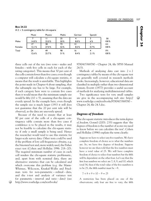
DEGREES OF FREEDOM 527
Box 24.22
A2× 5contingencytableforchi-square
Music Physics Maths German Spanish
7 11 25 4 3 50
Males 14.0 % 22.0 % 50 % 8.0 % 6% 100 %
17 38 73 12 1 141
Females 12.1 % 27.0 % 52 % 8.5 % 0.7 % 100 %
Total 24 49 98 16 4 191
12.6 % 25.7 % 51 % 8.4 % 2.1 % 100 %
Chapter 24
three cells out of the ten (two rows – males and
females – with five cells in each for each of the
rating categories). This means that 30 per cent of
the cells contain fewer than five cases; even though
acomputerwillcalculateachi-squarestatistic,it
means that the result is unreliable. This highlights
the point made in Chapter 4 about sampling, that
the subsample size has to be large. For example,
if each category here were to contain five cases
then it would mean that the minimum sample size
would be fifty (10 × 5), assuming that the data are
evenly spread. In the example here, even though
the sample size is much larger (191) it still does
not guarantee that the 20 per cent rule will be
observed, as the data are unevenly spread.
Because of the need to ensure that at least
80 per cent of the cells of a chi-square contingency
table contain more than five cases if
confidence is to be placed in the results, it may
not be feasible to calculate the chi-square statistic
if only a small sample is being used. Hence
the researcher would tend to use this statistic for
larger-scale survey data. Other tests could be used
if the problem of low cell frequencies obtains, e.g.
the binomial test and, more widely used, the Fisher
exact test (Cohen and Holliday 1996: 218–20).
The required minimum number of cases in each
cell renders the chi-square statistic problematic,
and, apart from with nominal data, there are
alternative statistics that can be calculated and
which overcome this problem (e.g. the Mann-
Whitney, Wilcoxon, Kruskal-Wallis and Friedman
tests for non-parametric – ordinal – data,
and the t-test and analysis of variance test
for parametric – interval and ratio – data) (see
http://www.routledge.com/textbooks/
9780415368780 – Chapter 24, file SPSS Manual
24.5).
Methods of analysing data cast into 2 × 2
contingency tables by means of the chi-square test
are generally well covered in research methods
books. Increasingly, however, educational data are
classified in multiple rather than two-dimensional
formats. Everitt (1977) provides a useful account
of methods for analysing multidimensional tables.
Two significance tests for very small samples
are give in the accompanying web site: http://
www.routledge.com/textbooks/9780415368780 –
Chapter 24, file 24.3.doc.
Degrees of freedom
The chi-square statistic introduces the term degrees
of freedom.Gorard(2001:233)suggeststhat‘the
degrees of freedom is the number of scores we need
to know before we can calculate the rest’. Cohen
and Holliday (1996) explain the term clearly:
Suppose we have to select any five numbers. We have
complete freedom of choice as to what the numbers
are. So, we have five degrees of freedom. Suppose
however we are then told that the five numbers must
have a total value of 25. We will have complete
freedom of choice to select four numbers but the fifth
will be dependent on the other four. Let’s say that the
first four numbers we select are 7, 8, 9, and 10, which
total 34, then if the total value of the five numbers is
to be 25, the fifth number must be −9.
7 + 8 + 9 + 10 − 9 = 25
A restriction has been placed on one of the
observations; only four are free to vary; the fifth