Subdivision Surfaces
Subdivision Surfaces
Subdivision Surfaces

Create successful ePaper yourself
Turn your PDF publications into a flip-book with our unique Google optimized e-Paper software.
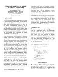
<strong>Subdivision</strong> ision Techniqueses<br />
Spring 2010<br />
1
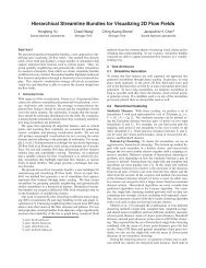
Curve Corner Cutting<br />
Take two points on different edges of a polygon and<br />
join them with a line segment. Then, use this line<br />
segment to replace all vertices and edges in between.<br />
This is corner cutting!<br />
Corner cutting can be local or non-local.<br />
A cut is localif it removes exactly one vertex and<br />
adds two new ones. Otherwise, it is non-local.<br />
all local cuts<br />
non-local cut<br />
2
Simple Corner Cutting: 1/5<br />
On each edge, choose two numbers u ≥ 0 and v ≥ 0<br />
and u+v ≤ 1, and divide the edge in the ratio of u:1-<br />
(u+v):v.<br />
u<br />
1-(u+v)<br />
v<br />
Here is how to cut a corner.<br />
3
Simple Corner Cutting: 2/5<br />
Suppose we have a polyline P 0 . Divide its edges<br />
with the above scheme, yielding a new polyline li P 1 .<br />
Dividing P 1 yields P 2 , …., and so on. What is<br />
P ∞ = Limit i P i<br />
i→∞<br />
The u’s and v’s do not have to be the same for every<br />
edge. Moreover, the u’s and v’s used to divide P i do<br />
not have to be equal to those u’s s andv’s v used to<br />
divide P i+1 .<br />
4
Simple Corner Cutting: 3/5<br />
1/4<br />
P 0<br />
u = 1/3 and v = 1/4<br />
P<br />
P 1<br />
P 2<br />
1/3<br />
5
Simple Corner Cutting: 4/5<br />
For a polygon, one more leg from the last point<br />
to the first must also be divided accordingly.<br />
u = 1/3 and v =1/4<br />
6
Simple Corner Cutting: 5/5<br />
1/2<br />
v<br />
1<br />
2u+v ≤ 1<br />
u+2v ≤ 1<br />
1<br />
1/2<br />
Chaikin used u = v = 1/4<br />
u<br />
The following result was proved<br />
by Gregory and Qu, de Boor,<br />
and Paluszny, Prautzsch and<br />
Schäfer.<br />
If all u’s and v’s lies in the<br />
interior of the area bounded by<br />
u ≥ 0, v ≥ 0, u+2v ≤ 1 and 2u+v ≤<br />
1, then P ∞ is a C 1 curve.<br />
This procedure was studied by<br />
Chaikin in 1974, and was later<br />
proved that the limit curve is a<br />
B-spline curve of degree 2.<br />
7
FYI<br />
<strong>Subdivision</strong> and refinement has its first significant<br />
use in Pixar’s Geri’sGame<br />
Game.<br />
Geri’s Game received the Academy Award for Best<br />
Animated Short Film in 1997.<br />
http://www.pixar.com/shorts/gg/<br />
8
Facts about <strong>Subdivision</strong> <strong>Surfaces</strong><br />
<strong>Subdivision</strong> surfaces are limit surfaces:<br />
‣It starts with a mesh<br />
‣It is then refined by repeated subdivision<br />
Since the subdivision process can be carried out<br />
infinite number of times, the intermediate<br />
meshes are approximations of the actual<br />
subdivision surface.<br />
<strong>Subdivision</strong> surfaces is a simple technique for<br />
describing complex surfaces of arbitrary<br />
topology with guaranteed continuity.<br />
Also supports Multiresolution.<br />
9
What Can You Expect from …<br />
It is easy to model a large number of surfaces<br />
of various types.<br />
Usually, it generates smooth surfaces.<br />
It has simple and intuitive interaction with<br />
models.<br />
It can model sharp and semi-sharp features of<br />
surfaces.<br />
Its representation is simple and compact (e.g.,<br />
winged-edge and half-edge data structures, etc).<br />
We only discuss 2-manifolds without boundary.<br />
10
Regular Quad Mesh <strong>Subdivision</strong>: 1/3<br />
Assume all faces in a mesh are quadrilaterals<br />
and each vertex has four adjacent faces.<br />
From the vertices C 1 1, C 2 2, C 3 and C 4 of a<br />
quadrilateral, four new vertices c 1 , c 2 , c 3 and c 4<br />
can be computed in the following way y( (mod 4):<br />
3 9 3 1<br />
c = C + C + C + C<br />
16 16 16 16<br />
i i− 1 i i+ 1 i+<br />
2<br />
If we define matrix Q as follows:<br />
⎡9 /16 3 /16 1/16 3 /16⎤<br />
⎢<br />
3 /16 9 /16 3 /16 1/16<br />
⎥<br />
Q= ⎢<br />
⎥<br />
⎢1/16 3 /16 9 /16 3 /16⎥<br />
⎢<br />
⎥<br />
⎣<br />
3 /16 1/16 3 /16 9 /16<br />
⎦<br />
11
Regular Quad Mesh <strong>Subdivision</strong>: 2/3<br />
Then, we have the following relation:<br />
⎡c1⎤ ⎡C1⎤<br />
⎢ ⎥ ⎢ ⎥<br />
⎢<br />
c2⎥ ⎢<br />
C2<br />
= Q ⋅ ⎥<br />
⎢c<br />
⎥ ⎢ 3<br />
C ⎥<br />
3<br />
⎢ ⎥ ⎢ ⎥<br />
⎣c4⎦ ⎣C4⎦<br />
C 4<br />
C 3<br />
c 4<br />
c 3<br />
c 1<br />
c 2<br />
C<br />
12<br />
C 1 C 2
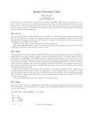
Regular Quad Mesh <strong>Subdivision</strong>: 3/3<br />
New vertices c 1 , c 2 , c 3 and c 4 of the current face<br />
are connected to the c i ’s of the neighboring<br />
faces to form new, smaller faces.<br />
The new mesh is still a quadrilateral mesh.<br />
original mesh<br />
new mesh<br />
this corner is cut!<br />
13
Arbitrary Grid Mesh<br />
If a vertex in a quadrilateral (resp., triangular)<br />
mesh is not adjacent to four (resp., six) neighbors,<br />
it is an extraordinary vertex.<br />
A non-regular quad or triangular mesh has<br />
extraordinary vertices and extraordinary faces.<br />
extraordinary vertices<br />
quad mesh<br />
triangular mesh<br />
14
Doo-Sabin <strong>Subdivision</strong>: 1/6<br />
Doo and Sabin, in 1978, suggested the following<br />
for computing c i ’s from C i ’s:<br />
c<br />
n<br />
= ∑α<br />
C<br />
i ij j<br />
j=<br />
1<br />
where α ij ’s are defined as follows:<br />
⎧ n + 5<br />
⎪<br />
i<br />
=<br />
j<br />
4 n<br />
⎪<br />
αij<br />
=⎨ ⎪<br />
⎪<br />
1 ⎡ ⎛2 π( i− j)<br />
⎞⎤<br />
3+ 2cos otherwise<br />
⎪<br />
⎜ ⎟<br />
4n<br />
⎢<br />
n<br />
⎥<br />
⎩ ⎣ ⎝ ⎠⎦<br />
15
Doo-Sabin <strong>Subdivision</strong>: 2/6<br />
F-face<br />
E-face<br />
V-facef<br />
There are three types<br />
of faces in the new<br />
mesh.<br />
A F-facef is obtained<br />
by connecting the c i ’s<br />
of a face.<br />
An E-face is obtained<br />
by connecting the c i’s<br />
of the faces that<br />
share an edge.<br />
A V-face is obtained<br />
by connecting the c i ’s<br />
that t surround a<br />
vertex.<br />
16
Doo-Sabin <strong>Subdivision</strong>: 3/6<br />
Most faces are quadrilaterals. None four-sided<br />
faces are those V-faces and converge to points<br />
whose valency is not four (i.e., extraordinary<br />
vertices).<br />
Thus, , a large portion of the limit surface are<br />
covered by quadrilaterals, and the surface is mostly<br />
a B-spline surfaces of degree (2,2). However, it is<br />
only G 1 everywhere.<br />
17
Doo-Sabin <strong>Subdivision</strong>: 4/6<br />
1 2 3<br />
18<br />
4 5 6
Doo-Sabin <strong>Subdivision</strong>: 5/6<br />
1 2 3<br />
4 5<br />
19
Doo-Sabin <strong>Subdivision</strong>: 6/6<br />
1 2 3<br />
4 5<br />
20
Catmull-Clark Algorithm: 1/10<br />
Catmull and Clark proposed another algorithm<br />
in the same year as Doo and Sabin did (1978).<br />
In fact, both papers p appeared in the journal<br />
Computer-Aided Design back to back!<br />
Catmull-Clark’s Clark s algorithm is rather complex. It<br />
computes a face point for each face, followed by<br />
an edge point for each edge, and then a vertex<br />
point for each vertex.<br />
Once these new points are available, a new mesh<br />
is constructed.<br />
21
Catmull-Clark Algorithm: 2/10<br />
Compute a face point for each face. This face<br />
point is the gravity center or centroid of the face,<br />
which is the average of all vertices of that face:<br />
22
Catmull-Clark Algorithm: 3/10<br />
Compute an edge point for each edge. An edge point is<br />
the average of the two endpoints of that edge and the two<br />
face points of that edge’s adjacent faces.<br />
23
Catmull-Clark Algorithm: 4/10<br />
Compute a vertex point for each vertex v as<br />
follows:<br />
' 1 2 n − 3<br />
v =<br />
Q+ R+ v<br />
n n n<br />
m<br />
f<br />
Q – the average of all new face<br />
1<br />
2<br />
Q points of v<br />
R – the average of all mid-points<br />
f (i.e., m i ’s) of vertex v<br />
1 v<br />
m 3<br />
v - the original vertex<br />
n - # of incident edges of v<br />
m 2<br />
3<br />
g<br />
R<br />
f 3<br />
24
Catmull-Clark Algorithm: 5/10<br />
For each face, connect its face point f to each<br />
edge point, and connect each new vertex v ’ to the<br />
two edge points of the edges incident to v.<br />
e<br />
f<br />
25
Catmull-Clark Algorithm: 6/10<br />
face point<br />
edge point<br />
vertex point<br />
vertex-edge<br />
connection<br />
26<br />
face-edge connection
Catmull-Clark Algorithm: 7/10<br />
After the first run, all faces are four sided.<br />
If all faces are four-sided, each has four edge points e 1 , e 2 , e 3<br />
and e 4 , four vertices v 1 , v 2 , v 3 and v 4 , and one new vertex v.<br />
Their relation can be represented as follows:<br />
A vertex at any level converges to the following:<br />
∑<br />
∑<br />
4<br />
4 4<br />
j= 1 j j=<br />
1 j<br />
2<br />
n + +<br />
v = v e f<br />
∞<br />
nn ( + 5)<br />
The limit surface is a B-spline surface of degree (3,3).<br />
27
Catmull-Clark Algorithm: 8/10<br />
1 2 3<br />
4 5 6<br />
28
Catmull-Clark Algorithm: 9/10<br />
1 2 3<br />
4 5<br />
29
Catmull-Clark Algorithm: 10/10<br />
1 2 3<br />
30<br />
4 5
Loop’s Algorithm: 1/6<br />
Loop’s (i.e., Charles Loop’s) algorithm only<br />
works for triangle meshes.<br />
Loop’s p algorithm computes a new edge point<br />
for each edge and a new vertex for each vertex.<br />
Let v 1 v 2 be an edge and the other vertices of<br />
the incident triangles be v left and v right . The<br />
new edge point e is computed as follows.<br />
e= 3 v v 1 v v<br />
8 8<br />
( + ) + ( + )<br />
1 2 left right<br />
1<br />
v left<br />
3<br />
3<br />
v 1<br />
v 2<br />
1<br />
v right<br />
31
Loop’s Algorithm: 2/6<br />
For each vertex v, its new vertex point v’ is<br />
computed below, where v 1 , v 2 , …, v n are<br />
adjacent vertices<br />
n<br />
'<br />
v = (1 − nα)<br />
v+ α∑<br />
v<br />
j<br />
j=<br />
1<br />
1-nα<br />
where α is α α<br />
⎧<br />
⎪ 3 n=<br />
⎪16<br />
3<br />
⎪<br />
α =⎨⎨<br />
⎪ 2<br />
⎪15 ⎡ ⎛3 1 2π<br />
⎞ ⎤<br />
− + cos n><br />
3<br />
⎪<br />
⎢ ⎜ ⎟ ⎥<br />
⎩<br />
n<br />
⎢⎣<br />
8 ⎝ 8 4<br />
n<br />
⎠<br />
⎥⎦<br />
α<br />
α<br />
α<br />
32
Loop’s Algorithm: 3/6<br />
Let a triangle be defined by<br />
X 1 , X 2 and X 3 and the<br />
v 1 corresponding new vertex<br />
points be v 1 , v 2 and v 3 .<br />
X 1 e 2<br />
Let the edge points of edges<br />
e v 1 v 2 , v 2 v 3 and v 3 v 1 be e 3 , e 1<br />
3<br />
and e 2 . The new triangles<br />
e 1<br />
are v 1e 2e 3 3, v 2e 3e 1 1, v 3e 1e 2 and<br />
X<br />
v<br />
2<br />
3 e 1 e 2 e 3 . This is a 1-to-4<br />
X 3<br />
scheme.<br />
This algorithm was<br />
developed by Charles Loop<br />
in 1987.<br />
v 2<br />
33
Loop’s Algorithm: 4/6<br />
Pick a vertex in the original or an intermediate<br />
mesh. If this vertex has n adjacent vertices v 1 ,<br />
v 2 , …, v n , it converges to v ∞ :<br />
n<br />
3+ 8( n −1) α 8α<br />
v∞<br />
= + ∑ v<br />
j<br />
3 + 8 n<br />
α 3 +<br />
8 n<br />
α j =<br />
1<br />
If all vertices have valency 6, the limit surface is<br />
a collection of C 2 Bézier triangles.<br />
However, only a torus can be formed with all<br />
valency 6 vertices. Vertices with different<br />
valencies converge to extraordinary vertices<br />
where the surface is only G 1 .<br />
34
Loop’s Algorithm: 5/6<br />
Doo-Sabin<br />
Catmull-Clark 35
Loop’s Algorithm: 6/6<br />
Doo-Sabin<br />
36<br />
Catmull-Clark
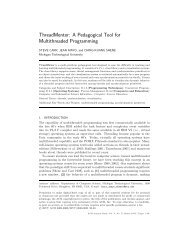
Peters-Reif Algorithm: 1/4<br />
This is an extremely simple<br />
algorithm.<br />
Compute the midpoint<br />
of each edge<br />
For each face, create a<br />
face by connecting the<br />
midpoints of it edges<br />
There are two types of faces:<br />
faces inscribed to the<br />
existing ones and faces<br />
whose vertices are the<br />
midpoints of edges that are<br />
incident to a common<br />
vertex.<br />
37
Peters-Reif Algorithm: 2/4<br />
The original and new vertices has a<br />
relationship as follows:<br />
⎡1 1<br />
⎢2 ⎢<br />
2<br />
<br />
<br />
⎤<br />
0<br />
⎥<br />
⎥<br />
'<br />
⎡ v<br />
⎤<br />
1 1 1<br />
⎡ 1<br />
⎤<br />
⎢ ' ⎥ ⎢0 0⎥<br />
⎢ ⎥<br />
v2<br />
⎢<br />
⎥ v2<br />
⎢ ⎥ 2 2 ⎢ ⎥<br />
⎢ ⎢<br />
⎥<br />
⎥ = ⎢ ⎥<br />
⎢<br />
<br />
⎥<br />
⋅ <br />
⎢<br />
'<br />
⎥ ⎢ ⎥<br />
⎢ v<br />
1 1<br />
n−1<br />
⎥ ⎢ ⎥<br />
1<br />
0<br />
⎢vn−<br />
⎥<br />
' ⎢ <br />
⎢ ⎥ ⎥<br />
2 2 ⎢ ⎥<br />
⎣ vn<br />
⎦ ⎢ ⎥ ⎣ vn<br />
⎦<br />
⎢1 1⎥<br />
⎢<br />
0 0<br />
⎣2 2⎥⎦<br />
v<br />
The limit of this process consists of a set of<br />
regular planar polygons that are the tangent<br />
planes of the limit surface, which is G 1 .<br />
Peters-Reif algorithm was developed by J.<br />
Peters and U. Reif in 1998.<br />
38
Peters-Reif Algorithm: 3/4<br />
39
Peters-Reif Algorithm: 4/4<br />
Doo-Sabin<br />
Catmull-Clark 40
√3-<strong>Subdivision</strong> of Kobbelt: 1/8<br />
<br />
<br />
This algorithm was developed by Leif<br />
Kobbelt in 2000, and only works for triangle<br />
meshes.<br />
This simple algorithm consists of three steps:<br />
1) Dividing each triangle at the center into 3<br />
more triangles<br />
2) Perturb the vertices of each triangle<br />
3) “Flip” the edges of the perturbed triangle<br />
(see next slide).<br />
41
√3-<strong>Subdivision</strong> of Kobbelt: 2/8<br />
Step 1: Subdividing<br />
new edge<br />
V 1<br />
<br />
For each triangle,<br />
compute its center:<br />
C = (V 1 +V 2 +V 3 )/3<br />
C<br />
Connect the center<br />
to each vertex to<br />
create 3 triangles.<br />
This is a 1-to-3<br />
scheme!<br />
42
√3-<strong>Subdivision</strong> of Kobbelt: 3/8<br />
Step 2: Flipping Edges<br />
<br />
Since each original<br />
edge is adjacent to<br />
two triangles,<br />
“flipping” an edge<br />
means removing the<br />
original edge and<br />
replacing it by the<br />
new edge joining<br />
the centers.<br />
Dotted: original Solid: “flipped”<br />
43
√3-<strong>Subdivision</strong> of Kobbelt: 4/8<br />
Final Result<br />
<br />
<br />
Remove the<br />
original edges and<br />
we have a new<br />
triangle mesh!<br />
But, the original<br />
vertices must also<br />
be “perturbed” a<br />
little to preserve<br />
“smoothness”.<br />
44
√3-<strong>Subdivision</strong> S ision of Kobbelt: 5/8<br />
Actual Computation<br />
For each triangle with vertices V 1 , V 2 and V 3 ,<br />
<br />
<br />
compute its center C:<br />
1<br />
C= ( V1+<br />
V<br />
2<br />
+V3)<br />
3<br />
For each vertex V and its neighbors V 1 1, V 2 2, …,<br />
V n , compute a perturbed V’ as follows:<br />
α<br />
n<br />
'<br />
n<br />
V = ( 1− α<br />
n<br />
) V+ ∑ V<br />
i<br />
n i = 1<br />
where α n is computed as follows:<br />
1 ⎛<br />
⎛2ππ<br />
⎞<br />
⎞<br />
αn<br />
= 4 2cos<br />
9<br />
⎜ − ⎜ ⎟<br />
n<br />
⎟<br />
⎝ ⎝ ⎠⎠<br />
Replace V i ’s with V’ i ’s and do edge flipping.<br />
45
√3-<strong>Subdivision</strong> of Kobbelt: 6/8<br />
Important Results<br />
<br />
<br />
<br />
<br />
The √3-subdivision converges!<br />
The limit surface is C 2 everywhere except for<br />
extraordinary ypoints.<br />
It is only C 1 at extraordinary points (i.e.,<br />
vertices with valance ≠ 6).<br />
The √3-subdivision can be extended to an<br />
adaptive scheme for finer subdivision control.<br />
46
√3-<strong>Subdivision</strong> of Kobbelt: 7/8<br />
1 2 3<br />
2<br />
4 5 5 rendered<br />
d<br />
47
√3-<strong>Subdivision</strong> of Kobbelt: 8/8<br />
1 2 3<br />
48<br />
4 5 5 rendered
The End<br />
49