Adobe PDF

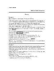
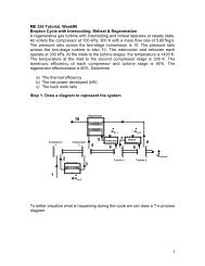
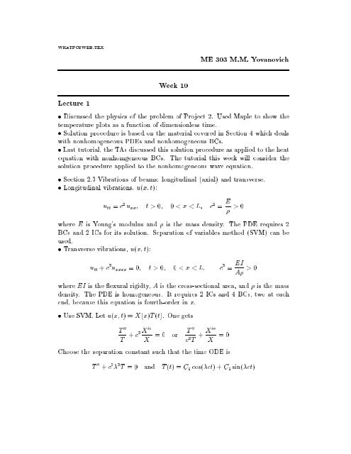
WKxTPCSWEB.TEX
ME 303 M.M. Yovanovich
Week 10
Lecture 1
Discussed the physics of the problem of Project 2. Used Maple to show the
temperature plots as a function of dimensionless time.
Solution procedure is based on the material covered in Section 4 which deals
with nonhomogeneous PDEs and nonhomogeneous BCs.
Last tutorial, the TAs discussed this solution procedure as applied to the heat
equation with nonhomgeneous BCs. The tutorial this week will consider the
solution procedure applied to the nonhomogeneous wave equation.
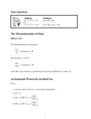
Section 2.3 Vibrations of beams: longitudinal (axial) and transverse.
Longitudinal vibrations, u(x; t):
u tt = c 2 u xx ; t>0; 0

The spatial ODE becomes:
X iv , m 4 X =0;
0

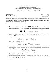
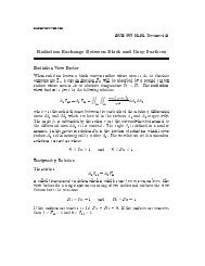
where h is the heat transfer coecient, and T 1 is the ambient temperature. An
energy balance (heat balance) at the end x = L where Q cond = Q conv gives
the Robin BC: !
@u(x; t)
= , h @x
k (u(L; t) , T 1)
x=L
This BC is nonhomogeneous due to T 1 . It can be made homogeneous by the
introduction of (x; t) =u(x; t) , T 1 . Note that
The Robin condition becomes:
@
@x = @u
@x ; because @T 1
@x =0
@(x; t)
@x
!
x=L
= , h k (L)
which is homogeneous.
Observe that Spiegel has used the symbol h to represent the two parameters
h=k. Many math texts do this. Be careful of the units.
Lecture 2
Alternative formulation of the problem of Section 4.5.
and
@ 2
@x = 1 @
; t>0; 0

Since C 2 = 0 gives a trivial solution we choose
cos L + h sin L =0 or cos + Bi sin =0
k
where = L and Bi = hL=k with 0

This is a Fourier sine series. The Fourier coecients D n can be found by means
of the orthogonality property of the sines. Multipy the left-hand side and all
terms of the right-hand side by sin m xdxand integrate with respect to x. Thus
Z L
When m 6= n wehave
0
otherwise when m = n ,
Z L
0
(f(x) , T 1 ) sin m xdx=
Z L
0
1X
n=1
sin m x sin n xdx=0
sin 2 n xdx= nL , cos n L sin n L
2 n
= L 2
Z L
D n sin m x sin n xdx
0
" #
n , cos n sin n
n
Using the relationship given by the CE, the above integral can be written as
Z L
and the Fourier coecients are given by
D n =
0
sin 2 n xdx= L Bi + cos 2 n
2 Bi
Bi 2
Bi + cos 2 n L
Z L
0
(f(x) , T 1 ) sin n xdx
To proceed further one needs to specify the function f(x).
Lecture 3
Similarity Method (Boltzmann Transformation)
Transforms PDE into ODE.
One-dimensional diusion equation:
with initial condition:
and boundary conditions for t>0:
T xx = 1 T t; t>0; x>0
T (x; 0) = T i ; x 0
T (0;t)=T 0 ;
T (x !1;t) ! T i
5

Dene temperature excess to create homogeneous conditions: (x; t) =T (x; t),
T i . The problem becomes:
with initial condition:
and boundary conditions for t>0:
xx = 1 t; t>0; x>0
(x; 0)=0; x 0
(0;t)= 0 = T 0 , T i ; (x !1;t) ! 0
Introduce the similarity parameter: =
@
@x = p 1 and @
4t @t =
Let () =(x; t)= 0 .
Transform the partial derivatives.
@
@x = @
@ [ 0] @
@ 2
@x = @ @
2 @x @x = @
@
@
@t = @ @ ( 0 ) @
@t = @ @
0
@ @t
Substitute into the PDE and replace
x p
4t
. Note that
p x , 1
4 2 t,3=2
@x = 0 @
p
4t @
(
0 @ p4t
@
)
@
@x = 0 @ 2
4t @ 2
( )
x
p t ,1=2 = x 0
p , 1 @
4 4 2 t,3=2 @ =
, x p 0 @
2t 4t @ = , 0 @
2t @
@ 2
@ 2
by
d 2
because () only
d 2
@ 2
@x 2 , 1
@
@t = 0 d 2
4t d + 0 d
2 2t d =0
Divide by 0 and multiply by 4t to get ODE:
d 2
d 2 +2 d =0
6

Transformed initial and boundary conditions:
and
t =0; = 1; =0
t>0; x =0; =0; =1
t>0; x !1; !1; ! 0
Solution of ODE.
Let w = d=d to reduce order of ODE.
dw
d
+2w =0
Apply separation of variables method to nd the solution of the ODE. Therefore,
dw
w = ,2d
After integration we get
w = d
d = C 1e ,2
Another integration gives
Z
= C 1 e ,2 d + C 2
0
where lower limit was arbitrarily set to zero.
Apply the boundary conditions to nd the constants: C 1 ;C 2 . When =0,
= 1, the integral is zero, and C 2 =1.
When = 1, = 0 and we have
0=C 1
Z 1
0
e ,2 d +1=C 1
p
2 +1
The value of the integral is p =2. The rst constant ofintegration is
C 1 = , 2 p
The solution of the ODE and therefore the PDE is
=1, 2 p
Z
0
e ,2 d =1, erf() =erfc()
7

where erf() and erfc() are the error and complementary error functions with
similarity parameter: = x=(2 p t).
The solution can also be expressed as
T (x; t) , T i
= erfc
T 0 , T i
x
2 p t
!
t>0; x 0
See Maple worksheets for Similarity Method and some characteristics of the
error and complementary error functions.
Some properties of these important special functions:
erf(0)=0; erf(1) =1; erf(,) =,erf(); erfc() =1, erf()
8