
Create successful ePaper yourself
Turn your PDF publications into a flip-book with our unique Google optimized e-Paper software.
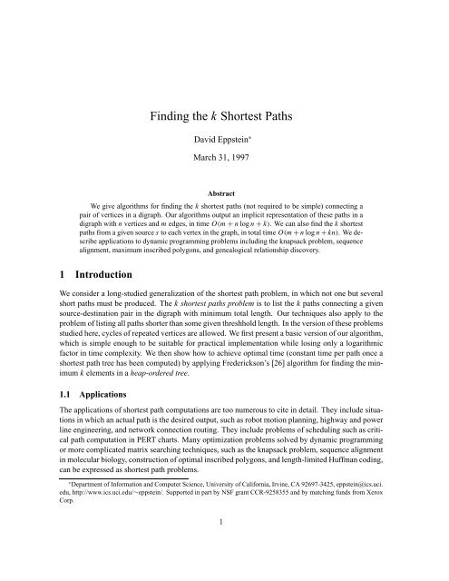
<strong>Finding</strong> <strong>the</strong> k <strong>Shortest</strong> <strong>Paths</strong><br />
David Eppstein ∗<br />
March 31, 1997<br />
Abstract<br />
We give algorithms for finding <strong>the</strong> k shortest paths (not required to be simple) connecting a<br />
pair of vertices in a digraph. Our algorithms output an implicit representation of <strong>the</strong>se paths in a<br />
digraph with n vertices and m edges, in time O(m + n log n + k). We can also find <strong>the</strong> k shortest<br />
paths from a given source s to each vertex in <strong>the</strong> graph, in total time O(m + n log n + kn). We describe<br />
applications to dynamic programming problems including <strong>the</strong> knapsack problem, sequence<br />
alignment, maximum inscribed polygons, and genealogical relationship discovery.<br />
1 Introduction<br />
We consider a long-studied generalization of <strong>the</strong> shortest path problem, in which not one but several<br />
short paths must be produced. The k shortest paths problem is to list <strong>the</strong> k paths connecting a given<br />
source-destination pair in <strong>the</strong> digraph with minimum total length. Our techniques also apply to <strong>the</strong><br />
problem of listing all paths shorter than some given threshhold length. In <strong>the</strong> version of <strong>the</strong>se problems<br />
studied here, cycles of repeated vertices are allowed. We first present a basic version of our algorithm,<br />
which is simple enough to be suitable for practical implementation while losing only a logarithmic<br />
factor in time complexity. We <strong>the</strong>n show how to achieve optimal time (constant time per path once a<br />
shortest path tree has been computed) by applying Frederickson’s [26] algorithm for finding <strong>the</strong> minimum<br />
k elements in a heap-ordered tree.<br />
1.1 Applications<br />
The applications of shortest path computations are too numerous to cite in detail. They include situations<br />
in which an actual path is <strong>the</strong> desired output, such as robot motion planning, highway and power<br />
line engineering, and network connection routing. They include problems of scheduling such as critical<br />
path computation in PERT charts. Many optimization problems solved by dynamic programming<br />
or more complicated matrix searching techniques, such as <strong>the</strong> knapsack problem, sequence alignment<br />
in molecular biology, construction of optimal inscribed polygons, and length-limited Huffman coding,<br />
can be expressed as shortest path problems.<br />
∗ Department of Information and Computer Science, University of California, Irvine, CA 92697-3425, eppstein@ics.uci.<br />
edu, http://www.ics.uci.edu/∼eppstein/. Supported in part by NSF grant CCR-9258355 and by matching funds from Xerox<br />
Corp.<br />
1
Methods for finding k shortest paths have been applied to many of <strong>the</strong>se applications, for several<br />
reasons.<br />
• Additional constraints. One may wish to find a path that satisfies certain constraints beyond<br />
having a small length, but those o<strong>the</strong>r constraints may be ill-defined or hard to optimize. For<br />
instance, in power transmission route selection [18], a power line should connect its endpoints<br />
reasonably directly, but <strong>the</strong>re may be more or less community support for one option or ano<strong>the</strong>r.<br />
A typical solution is to compute several short paths and <strong>the</strong>n choose among <strong>the</strong>m by considering<br />
<strong>the</strong> o<strong>the</strong>r criteria. We recently implemented a similar technique as a heuristic for <strong>the</strong> NP-hard<br />
problem of, given a graph with colored edges, finding a shortest path using each color at most<br />
once [20]. This type of application is <strong>the</strong> main motivation cited by Dreyfus [17] and Lawler [39]<br />
for k shortest path computations.<br />
• Model evaluation. <strong>Paths</strong> may be used to model problems that have known solutions, independent<br />
of <strong>the</strong> path formulation; for instance, in a k-shortest-path model of automatic translation<br />
between natural languages [30], a correct translation can be found by a human expert. By listing<br />
paths until this known solution appears, one can determine how well <strong>the</strong> model fits <strong>the</strong> problem,<br />
in terms of <strong>the</strong> number of incorrect paths seen before <strong>the</strong> correct path. This information can be<br />
used to tune <strong>the</strong> model as well as to determine <strong>the</strong> number of paths that need to be generated<br />
when applying additional constraints to search for <strong>the</strong> correct solution.<br />
• Sensitivity analysis. By computing more than one shortest path, one can determine how sensitive<br />
<strong>the</strong> optimal solution is to variation of <strong>the</strong> problem’s parameters. In biological sequence<br />
alignment, for example, one typically wishes to see several “good” alignments ra<strong>the</strong>r than one<br />
optimal alignment; by comparing <strong>the</strong>se several alignments, biologists can determine which portions<br />
of an alignment are most essential [8,64]. This problem can be reduced to finding several<br />
shortest paths in a grid graph.<br />
• Generation of alternatives. It may be useful to examine not just <strong>the</strong> optimal solution to a problem,<br />
but a larger class of solutions, to gain a better understanding of <strong>the</strong> problem. For example,<br />
<strong>the</strong> states of a complex system might be represented as a finite state machine, essentially just<br />
a graph, with different probabilities on each state transition edge. In such a model, one would<br />
likely want to know not just <strong>the</strong> chain of events most likely to lead to a failure state, but ra<strong>the</strong>r all<br />
chains having a failure probability over some threshhold. Taking <strong>the</strong> logarithms of <strong>the</strong> transition<br />
probabilities transforms this problem into one of finding all paths shorter than a given length.<br />
We later discuss in more detail some of <strong>the</strong> dynamic programming applications listed above, and<br />
show how to find <strong>the</strong> k best solutions to <strong>the</strong>se problems by using our shortest path algorithms. As<br />
well as improving previous solutions to <strong>the</strong> general k shortest paths problem, our results improve more<br />
specialized algorithms for finding length-bounded paths in <strong>the</strong> grid graphs arising in sequence alignment<br />
[8] and for finding <strong>the</strong> k best solutions to <strong>the</strong> knapsack problem [15].<br />
2
1.2 New Results<br />
We prove <strong>the</strong> following results. In all cases we assume we are given a digraph in which each edge has<br />
a non-negative length. We allow <strong>the</strong> digraph to contain self-loops and multiple edges. In each case<br />
<strong>the</strong> paths are output in an implicit representation from which simple properties such as <strong>the</strong> length are<br />
available in constant time per path. We may explicitly list <strong>the</strong> edges in any path in time proportional<br />
to <strong>the</strong> number of edges.<br />
• We find <strong>the</strong> k shortest paths (allowing cycles) connecting a given pair of vertices in a digraph,<br />
in time O(m + n log n + k).<br />
• We find <strong>the</strong> k shortest paths from a given source in a digraph to each o<strong>the</strong>r vertex, in time O(m +<br />
n log n + kn).<br />
We can also solve <strong>the</strong> similar problem of finding all paths shorter than a given length, with <strong>the</strong> same<br />
time bounds. The same techniques apply to digraphs with negative edge lengths but no negative cycles,<br />
but <strong>the</strong> time bounds above should be modified to include <strong>the</strong> time to compute a single source shortest<br />
path tree in such networks, O(mn) [6,23] or O(mn 1/2 log N) where all edge lengths are integers and N<br />
is <strong>the</strong> absolute value of <strong>the</strong> most negative edge length [29]. For a directed acyclic graph (DAG), with or<br />
without negative edge lengths, shortest path trees can be constructed in linear time and <strong>the</strong> O(n log n)<br />
term above can be omitted. The related problem of finding <strong>the</strong> k longest paths in a DAG [4] can be<br />
transformed to a shortest path problem simply by negating all edge lengths; we can <strong>the</strong>refore also solve<br />
it in <strong>the</strong> same time bounds.<br />
1.3 Related Work<br />
Many papers study algorithms for k shortest paths [3,5,7,9,13,14,17,24,31,32,34,35,37–41,43–45,<br />
47, 50, 51, 56–60, 63, 65–69]. Dreyfus [17] and Yen [69] cite several additional papers on <strong>the</strong> subject<br />
going back as far as 1957.<br />
One must distinguish several common variations of <strong>the</strong> problem. In many of <strong>the</strong> papers cited above,<br />
<strong>the</strong> paths are restricted to be simple, i.e. no vertex can be repeated. This has advantages in some applications,<br />
but as our results show this restriction seems to make <strong>the</strong> problem significantly harder. Several<br />
papers [3, 13, 17, 24, 41, 42, 58, 59] consider <strong>the</strong> version of <strong>the</strong> k shortest paths problem in which repeated<br />
vertices are allowed, and it is this version that we also study. Of course, for <strong>the</strong> DAGs that arise<br />
in many of <strong>the</strong> applications described above including scheduling and dynamic programming, no path<br />
can have a repeated vertex and <strong>the</strong> two versions of <strong>the</strong> problem become equivalent. Note also that in<br />
<strong>the</strong> application described earlier of listing <strong>the</strong> most likely failure paths of a system modelled by a finite<br />
state machine, it is <strong>the</strong> version studied here ra<strong>the</strong>r than <strong>the</strong> more common simple path version that one<br />
wants to solve.<br />
One can also make a restriction that <strong>the</strong> paths found be edge disjoint or vertex disjoint [61], or<br />
include capacities on <strong>the</strong> edges [10–12, 49], however such changes turn <strong>the</strong> problem into one more<br />
closely related to network flow.<br />
Fox [24] gives a method for <strong>the</strong> k shortest path problem based on Dijkstra’s algorithm which with<br />
more recent improvements in priority queue data structures [27] takes time O(m+kn log n); this seems<br />
3
to be <strong>the</strong> best previously known k-shortest-paths algorithm. Dreyfus [17] mentions <strong>the</strong> version of <strong>the</strong><br />
problem in which we must find paths from one source to each o<strong>the</strong>r vertex in <strong>the</strong> graph, and describes<br />
a simple O(kn 2 ) time dynamic programming solution to this problem. For <strong>the</strong> k shortest simple paths<br />
problem, <strong>the</strong> best known bound is O(k(m + n log n)) in undirected graphs [35] or O(kn(m + n log n))<br />
in directed graphs [39, again including more recent improvements in Dijkstra’s algorithm]. Thus all<br />
previous algorithms took time O(n log n) or more per path. We improve this to constant time per path.<br />
A similar problem to <strong>the</strong> one studied here is that of finding <strong>the</strong> k minimum weight spanning trees<br />
in a graph. Recent algorithms for this problem [21, 22, 25] reduce it to finding <strong>the</strong> k minimum weight<br />
nodes in a heap-ordered tree, defined using <strong>the</strong> best swap in a sequence of graphs. Heap-ordered tree<br />
selection has also been used to find <strong>the</strong> smallest interpoint distances or <strong>the</strong> nearest neighbors in geometric<br />
point sets [16]. We apply a similar tree selection technique to <strong>the</strong> k shortest path problem, however<br />
<strong>the</strong> reduction of k shortest paths to heap ordered trees is very different from <strong>the</strong> constructions in <strong>the</strong>se<br />
o<strong>the</strong>r problems.<br />
2 The Basic Algorithm<br />
<strong>Finding</strong> <strong>the</strong> k shortest paths between two terminals s and t has been a difficult enough problem to warrant<br />
much research. In contrast, <strong>the</strong> similar problem of finding paths with only one terminal s, ending<br />
anywhere in <strong>the</strong> graph, is much easier: one can simply use breadth first search. Maintain a priority<br />
queue of paths, initially containing <strong>the</strong> single zero-edge path from s to itself; <strong>the</strong>n repeatedly remove<br />
<strong>the</strong> shortest path from <strong>the</strong> priority queue, add it to <strong>the</strong> list of output paths, and add all one-edge extensions<br />
of that path to <strong>the</strong> priority queue. If <strong>the</strong> graph has bounded degree d, a breadth first search from<br />
s until k paths are found takes time O(dk + k log k); note that this bound does not depend in any way<br />
on <strong>the</strong> overall size of <strong>the</strong> graph. If <strong>the</strong> paths need not be output in order by length, Frederickson’s heap<br />
selection algorithm [26] can be used to speed this up to O(dk).<br />
The main idea of our k shortest paths algorithm, <strong>the</strong>n, is to translate <strong>the</strong> problem from one with two<br />
terminals, s and t, to a problem with only one terminal. One can find paths from s to t simply by finding<br />
paths from s to any o<strong>the</strong>r vertex and concatenating a shortest path from that vertex to t. However we<br />
cannot simply apply this idea directly, for several reasons: (1) There is no obvious relation between <strong>the</strong><br />
ordering of <strong>the</strong> paths from s to o<strong>the</strong>r vertices, and of <strong>the</strong> corresponding paths from s to t. (2) Each path<br />
from s to t may be represented in many ways as a path from s to some vertex followed by a shortest<br />
path from that vertex to t. (3) Our input graph may not have bounded degree.<br />
In outline, we deal with problem (1) by using a potential function to modify <strong>the</strong> edge lengths in <strong>the</strong><br />
graph so that <strong>the</strong> length of any shortest path to t is zero; <strong>the</strong>refore concatenating such paths to paths<br />
from s will preserve <strong>the</strong> ordering of <strong>the</strong> path lengths. We deal with problem (2) by only considering<br />
paths from s in which <strong>the</strong> last edge is not in a fixed shortest path tree to t; this leads to <strong>the</strong> implicit<br />
representation we use to represent each path in constant space. (Similar ideas to <strong>the</strong>se appear also<br />
in [46].) However this solution gives rise to a fourth problem: (4) We do not wish to spend much time<br />
searching edges of <strong>the</strong> shortest path tree, as this time can not be charged against newly found s-t paths.<br />
The heart of our algorithm is <strong>the</strong> solution to problems (3) and (4). Our idea is to construct a binary<br />
heap for each vertex, listing <strong>the</strong> edges that are not part of <strong>the</strong> shortest path tree and that can be<br />
reached from that vertex by shortest-path-tree edges. In order to save time and space, we use persis-<br />
4
tence techniques to allow <strong>the</strong>se heaps to share common structures with each o<strong>the</strong>r. In <strong>the</strong> basic version<br />
of <strong>the</strong> algorithm, this collection of heaps forms a bounded-degree graph having O(m + n log n) vertices.<br />
Later we show how to improve <strong>the</strong> time and space bounds of this part of <strong>the</strong> algorithm using tree<br />
decomposition techniques of Frederickson [25].<br />
2.1 Preliminaries<br />
We assume throughout that our input graph G has n vertices and m edges. We allow self-loops and<br />
multiple edges so m may be larger than ( n<br />
2)<br />
. The length of an edge e is denoted l(e). By extension<br />
we can define <strong>the</strong> length l(p) for any path in G to be <strong>the</strong> sum of its edge lengths. The distance d(s, t)<br />
for a given pair of vertices is <strong>the</strong> length of <strong>the</strong> shortest path starting at s and ending at t; with <strong>the</strong> assumption<br />
of no negative cycles this is well defined. Note that d(s, t) may be unequal to d(t, s). The<br />
two endpoints of a directed edge e are denoted tail(e) and head(e); <strong>the</strong> edge is directed from tail(e) to<br />
head(e).<br />
For our purposes, a heap is a binary tree in which vertices have weights, satisfying <strong>the</strong> restriction<br />
that <strong>the</strong> weight of any vertex is less than or equal to <strong>the</strong> minimum weight of its children. We will not<br />
always care whe<strong>the</strong>r <strong>the</strong> tree is balanced (and in some circumstances we will allow trees with infinite<br />
depth). More generally, a D-heap is a degree-D tree with <strong>the</strong> same weight-ordering property; thus <strong>the</strong><br />
usual heaps above are 2-heaps. As is well known (e.g. see [62]), any set of values can be placed into<br />
a balanced heap by <strong>the</strong> heapify operation in linear time. In a balanced heap, any new element can be<br />
inserted in logarithmic time. We can list <strong>the</strong> elements of a heap in order by weight, taking logarithmic<br />
time to generate each element, simply by using breadth first search.<br />
2.2 Implicit Representation of <strong>Paths</strong><br />
As discussed earlier, our algorithm does not output each path it finds explicitly as a sequence of edges;<br />
instead it uses an implicit representation, described in this section.<br />
The ith shortest path in a digraph may have (ni) edges, so <strong>the</strong> best time we could hope for in an<br />
explicit listing of shortest paths would be O(k 2 n). Our time bounds are faster than this, so we must<br />
use an implicit representation for <strong>the</strong> paths. However our representation is not a serious obstacle to<br />
use of our algorithm: we can list <strong>the</strong> edges of any path we output in time proportional to <strong>the</strong> number of<br />
edges, and simple properties (such as <strong>the</strong> length) are available in constant time. Similar implicit representations<br />
have previously been used for related problems such as <strong>the</strong> k minimum weight spanning<br />
trees [21, 22, 25]. Fur<strong>the</strong>r, previous papers on <strong>the</strong> k shortest path problem give time bounds omitting<br />
<strong>the</strong> O(k 2 n) term above, and so <strong>the</strong>se papers must tacitly or not be using an implicit representation.<br />
Our representation is similar in spirit to those used for <strong>the</strong> k minimum weight spanning trees problem:<br />
for that problem, each successive tree differs from a previously listed tree by a swap, <strong>the</strong> insertion<br />
of one edge and removal of ano<strong>the</strong>r edge. The implicit representation consists of a pointer to <strong>the</strong> previous<br />
tree, and a description of <strong>the</strong> swap. For <strong>the</strong> shortest path problem, each successive path will turn<br />
out to differ from a previously listed path by <strong>the</strong> inclusion of a single edge not part of a shortest path<br />
tree, and appropriate adjustments in <strong>the</strong> portion of <strong>the</strong> path that involves shortest path tree edges. Our<br />
implicit representation consists of a pointer to <strong>the</strong> previous path, and a description of <strong>the</strong> newly added<br />
edge.<br />
5
s<br />
2<br />
20<br />
14<br />
55<br />
56<br />
36<br />
22<br />
13<br />
27<br />
14<br />
15<br />
9<br />
10<br />
25<br />
42<br />
33<br />
23<br />
7<br />
15 20<br />
12<br />
7<br />
18<br />
8<br />
11<br />
t<br />
37<br />
19<br />
11<br />
0<br />
Figure 1. (a) Example digraph G with edge lengths and specified terminals; (b) <strong>Shortest</strong> path tree T and distances<br />
to t in G.<br />
s<br />
3<br />
s<br />
3<br />
4<br />
1<br />
4<br />
9<br />
9<br />
10 6<br />
t<br />
t<br />
Figure 2. (a) Edges in G − T labeled by δ(e) (δ(e) = 0 for edges in T ); (b) Path p, sidetracks(p) (<strong>the</strong> heavy<br />
edges, labeled 3, 4, and 9), and prefpath(p) (differing from p in <strong>the</strong> two dashed edges; sidetracks(prefpath(p))<br />
consists of <strong>the</strong> two edges labeled 3 and 4).<br />
Given s and t in a digraph G (Figure 1(a)), let T be a single-destination shortest path tree with t as<br />
destination (Figure 1(b); this is <strong>the</strong> same as a single source shortest path tree in <strong>the</strong> graph G R formed<br />
by reversing each edge of G). We can compute T in time O(m +n log n) [27]. We denote by next T (v)<br />
<strong>the</strong> next vertex reached after v on <strong>the</strong> path from v to t in T .<br />
Given an edge e in G, define<br />
δ(e) = l(e) + d(head(e), t) − d(tail(e), t).<br />
Intuitively, δ(e) measures how much distance is lost by being “sidetracked” along e instead of taking<br />
a shortest path to t. The values of δ for our example graph are shown in Figure 2(a).<br />
Lemma 1. For any e ∈ G, δ(e) ≥ 0. For any e ∈ T , δ(e) = 0.<br />
For any path p in G, formed by a sequence of edges, some edges of p may be in T , and some<br />
o<strong>the</strong>rs may be in G − T . Any path p from s to t is uniquely determined solely by <strong>the</strong> subsequence<br />
sidetracks(p) of its edges in G − T (Figure 2(b)). For, given a pair of edges in <strong>the</strong> subsequence, <strong>the</strong>re<br />
is a uniquely determined way of inserting edges from T so that <strong>the</strong> head of <strong>the</strong> first edge is connected<br />
to <strong>the</strong> tail of <strong>the</strong> second edge. As an example, <strong>the</strong> shortest path in T from s to t is represented by <strong>the</strong><br />
6
empty sequence. A sequence of edges in G − T may not correspond to any s-t path, if it includes a<br />
pair of edges that cannot be connected by a path in T .IfS = sidetracks(p), we define path(S) to be<br />
<strong>the</strong> path p.<br />
Our implicit representation will involve <strong>the</strong>se sequences of edges in G − T . We next show how to<br />
recover l(p) from information in sidetracks(p).<br />
For any nonempty sequence S of edges in G − T , let prefix(S) be <strong>the</strong> sequence formed by <strong>the</strong> removal<br />
of <strong>the</strong> last edge in S. IfS = sidetracks(p), <strong>the</strong>n we denote this last sidetrack edge by lastsidetrack(p);<br />
prefix(S) will define a path prefpath(p) = path(prefix(S)) (Figure 2(b)).<br />
Lemma 2. For any path p from s to t,<br />
∑<br />
l(p) = d(s, t) +<br />
δ(e) = d(s, t) + ∑ δ(e).<br />
e∈sidetracks(p) e∈p<br />
Lemma 3. For any path p from s to t in G, for which sidetracks(p) is nonempty, l(p) ≥ l(prefpath(p)).<br />
Our representation of a path p in <strong>the</strong> list of paths produced by our algorithm will <strong>the</strong>n consist of<br />
two components:<br />
• The position in <strong>the</strong> list of prefpath(p).<br />
• Edge lastsidetrack(p).<br />
Although <strong>the</strong> final version of our algorithm, which uses Frederickson’s heap selection technique, does<br />
not necessarily output paths in sorted order, we will never<strong>the</strong>less be able to guarantee that prefpath(p)<br />
is output before p. One can easily recover p itself from our representation in time proportional to <strong>the</strong><br />
number of edges in p. The length l(p) for each path can easily be computed as δ(lastsidetrack(p)) +<br />
l(prefpath(p)). We will see later that we can also compute many o<strong>the</strong>r simple properties of <strong>the</strong> paths,<br />
in constant time per path.<br />
2.3 Representing <strong>Paths</strong> by a Heap<br />
The representation of s-t paths discussed in <strong>the</strong> previous section gives a natural tree of paths, in which<br />
<strong>the</strong> parent of any path p is prefpath(p) (Figure 3). The degree of any node in this path tree is at most<br />
m, since <strong>the</strong>re can be at most one child for each possible value of lastsidetrack(p). The possible values<br />
of lastsidetrack(q) for paths q that are children of p are exactly those edges in G − T that have tails<br />
on <strong>the</strong> path from head(lastsidetrack(p)) to t in <strong>the</strong> shortest path tree T .<br />
If G contains cycles, <strong>the</strong> path tree is infinite. By Lemma 3, <strong>the</strong> path tree is heap-ordered. However<br />
since its degree is not necessarily constant, we cannot directly apply breadth first search (nor Frederickson’s<br />
heap selection technique, described later in Lemma 8) to find its k minimum values. Instead<br />
we form a heap by replacing each node p of <strong>the</strong> path tree with an equivalent bounded-degree subtree<br />
(essentially, a heap of <strong>the</strong> edges with tails on <strong>the</strong> path from head(lastsidetrack(p)) to t, ordered by<br />
δ(e)). We must also take care that we do this in such a way that <strong>the</strong> portion of <strong>the</strong> path tree explored<br />
by our algorithm can be easily constructed.<br />
7
{}<br />
{3}<br />
{6} {10}<br />
{3,1} {3,4}<br />
{3,1,9}<br />
{3,4,6} {3,4,9}<br />
Figure 3. Tree of paths, labeled by sidetracks(p).<br />
For each vertex v we wish to form a heap H G (v) for all edges with tails on <strong>the</strong> path from v to t,<br />
ordered by δ(e). We will later use this heap to modify <strong>the</strong> path tree by replacing each node p with a<br />
copy of H G (head(lastsidetrack(p))).<br />
Let out(v) denote <strong>the</strong> edges in G − T with tails at v (Figure 4(a)). We first build a heap Hout(v),<br />
for each vertex v, of <strong>the</strong> edges in out(v) (Figure 4(b)). The weights used for <strong>the</strong> heap are simply <strong>the</strong><br />
values δ(e) defined earlier. Hout(v) will be a 2-heap with <strong>the</strong> added restriction that <strong>the</strong> root of <strong>the</strong> heap<br />
only has one child. It can be built for each v in time O(|out(v)|) by letting <strong>the</strong> root outroot(v) be <strong>the</strong><br />
edge minimizing δ(e) in out(v), and letting its child be a heap formed by heapification of <strong>the</strong> rest of<br />
<strong>the</strong> edges in out(v). The total time for this process is ∑ O(|out(v)|) = O(m).<br />
We next form <strong>the</strong> heap H G (v) by merging all heaps Hout(w) for w on <strong>the</strong> path in T from v to<br />
t. More specifically, for each vertex v we merge Hout(v) into H G (next T (v)) to form H G (v). We will<br />
continue to need H G (next T (v)), so this merger should be done in a persistent (nondestructive) fashion.<br />
We guide this merger of heaps using a balanced heap H T (v) for each vertex v, containing only<br />
<strong>the</strong> roots outroot(w) of <strong>the</strong> heaps Hout(w), for each w on <strong>the</strong> path from v to t. H T (v) is formed by<br />
inserting outroot(v) into H T (next T (v)) (Figure 5(a)). To perform this insertion persistently, we create<br />
new copies of <strong>the</strong> nodes on <strong>the</strong> path updated by <strong>the</strong> insertion (marked by asterisks in Figure 5(a)), with<br />
appropriate pointers to <strong>the</strong> o<strong>the</strong>r, unchanged, members of H T (next T (v)). Thus we can store H T (v)<br />
without changing H T (next T (v)), by using an additional O(log n) words of memory to store only <strong>the</strong><br />
nodes on that path.<br />
We now form H G (v) by connecting each node outroot(w) in H T (v) to an additional subtree beyond<br />
<strong>the</strong> two it points to in H T (v), namely to <strong>the</strong> rest of heap Hout(w). H G (v) can be constructed at <strong>the</strong><br />
same time as we construct H T (v), with a similar amount of work. H G (v) is thus a 3-heap as each node<br />
includes at most three children, ei<strong>the</strong>r two from H T (v) and one from Hout(w), or none from H T (v)<br />
and two from Hout(w).<br />
We summarize <strong>the</strong> construction so far, in a form that emphasizes <strong>the</strong> shared structure in <strong>the</strong> various<br />
heaps H G (v).<br />
Lemma 4. In time O(m + n log n) we can construct a directed acyclic graph D(G), and a map from<br />
vertices v ∈ G to h(v) ∈ D(G), with <strong>the</strong> following properties:<br />
8
p<br />
1<br />
6<br />
12<br />
14<br />
1<br />
6<br />
12 14<br />
q<br />
13<br />
3<br />
13 3<br />
s<br />
7<br />
17<br />
7<br />
r<br />
t<br />
17<br />
19<br />
4<br />
8<br />
10<br />
19<br />
4<br />
10<br />
8<br />
Figure 4. (a) Portion of a shortest path tree, showing out(v) and corresponding values of δ; (b) Hout(v).<br />
17*<br />
4*<br />
1*<br />
13<br />
p<br />
q<br />
1<br />
4<br />
4 6<br />
17 12 14<br />
13<br />
4*<br />
s<br />
3<br />
17<br />
13*<br />
4*<br />
17<br />
3*<br />
4*<br />
r<br />
4<br />
4<br />
17<br />
7<br />
19<br />
17*<br />
4*<br />
t 4<br />
10<br />
8<br />
Figure 5. (a) H T (v) with asterisks marking path of nodes updated by insertion of outroot(v) into H T (next T (v));<br />
(b) D(G) has a node for each marked node in Figure 5(a) and each non-root node in Figure 4(b).<br />
9
• D(G) has O(m + n log n) vertices.<br />
• Each vertex in D(G) corresponds to an edge in G − T .<br />
• Each vertex in D(G) has out-degree at most 3.<br />
• The vertices reachable in D(G) from h(v) form a 3-heap H G (v) in which <strong>the</strong> vertices of <strong>the</strong> heap<br />
correspond to edges of G − T with tails on <strong>the</strong> path in T from v to t, in heap order by <strong>the</strong> values<br />
of δ(e).<br />
Proof: The vertices in D(G) come from two sources: heaps Hout(v) and H T (v). Each node in Hout(v)<br />
corresponds to a unique edge in G−T , so <strong>the</strong>re are at most m−n+1 nodes coming from heaps Hout(v).<br />
Each vertex of G also contributes ⌊log 2 i⌋ nodes from heaps H T (v), where i is <strong>the</strong> length of <strong>the</strong> path<br />
from <strong>the</strong> vertex to t,1+⌊log 2 i⌋ measures <strong>the</strong> number of balanced binary heap nodes that need to be<br />
updated when inserting outroot(v) into H T (next T (v)), and we subtract one because outroot(v) itself<br />
was already included in our total for Hout(v). In <strong>the</strong> worst case, T is a path and <strong>the</strong> total contribution<br />
is at most ∑ i ⌊log 2 i⌋≤n log 2 n − cn where c varies between roughly 1.91 and 2 depending on<br />
<strong>the</strong> ratio of n to <strong>the</strong> nearest power of two. Therefore <strong>the</strong> total number of nodes in D(G) is at most<br />
m + n log 2 n − (c + 1)n. The degree bound follows from <strong>the</strong> construction, and it is straightforward to<br />
construct D(G) as described above in constant time per node, after computing <strong>the</strong> shortest path tree T<br />
in time O(m + n log n) using Fibonacci heaps [27].<br />
Map h(v) simply takes v to <strong>the</strong> root of H G (v). For any vertex v in D(G), let δ(v) be a shorthand<br />
for δ(e) where e is <strong>the</strong> edge in G corresponding to v. By construction, <strong>the</strong> nodes reachable from h(v)<br />
are those in H T (v) toge<strong>the</strong>r with, for each such node w, <strong>the</strong> rest of <strong>the</strong> nodes in Hout(w); H T (v) was<br />
constructed to correspond exactly to <strong>the</strong> vertices on <strong>the</strong> path from v to t, and Hout(w) represents <strong>the</strong><br />
edges with tails at each vertex, so toge<strong>the</strong>r <strong>the</strong>se reachable nodes represent all edges with tails on <strong>the</strong><br />
path. Each edge (u,v)in D(G) ei<strong>the</strong>r corresponds to an edge in some H T (w) or some Hout(w), and<br />
in ei<strong>the</strong>r case <strong>the</strong> heap ordering for D(G) is a consequence of <strong>the</strong> ordering in <strong>the</strong>se smaller heaps. ✷<br />
D(G) is shown in Figure 5(b). The nodes reachable from s in D(G) form a structure H G (s) representing<br />
<strong>the</strong> paths differing from <strong>the</strong> original shortest path by <strong>the</strong> addition of a single edge in G − T .<br />
We now describe how to augment D(G) with additional edges to produce a graph which can represent<br />
all s-t paths, not just those paths with a single edge in G − T .<br />
We define <strong>the</strong> path graph P(G) as follows. The vertices of P(G) are those of D(G), with one<br />
additional vertex, <strong>the</strong> root r = r(s). The vertices of P(G) are unweighted, but <strong>the</strong> edges are given<br />
lengths. For each directed edge (u,v) in D(G), we create <strong>the</strong> edge between <strong>the</strong> corresponding vertices<br />
in P(G), with length δ(v) − δ(u). We call such edges heap edges. For each vertex v in P(G),<br />
corresponding to an edge in G − T connecting some pair of vertices u and w, we create a new edge<br />
from v to h(w) in P(G), having as its length δ(h(w)). We call such edges cross edges. We also create<br />
an initial edge between r and h(s), having as its length δ(h(s)).<br />
P(G) has O(m +n log n) vertices, each with out-degree at most four. It can be constructed in time<br />
O(m + n log n).<br />
Lemma 5. There is a one-to-one length-preserving correspondence between s-t paths in G, and paths<br />
starting from r in P(G).<br />
10
Proof: Recall that an s-t path p in G is uniquely defined by sidetracks(p), <strong>the</strong> sequence of edges from<br />
p in G − T . We now show that for any such sequence, <strong>the</strong>re corresponds a unique path from r in<br />
P(G) ending at a node corresponding to lastsidetrack(p), and conversely any path from r in P(G)<br />
corresponds to sidetracks(p) for some path p.<br />
Given a path p in G, we construct a corresponding path p ′ in P(G) as follows. If sidetracks(p)<br />
is empty (i.e. p is <strong>the</strong> shortest path), we let p ′ consist of <strong>the</strong> single node r. O<strong>the</strong>rwise, form a path q ′<br />
in P(G) corresponding to prefpath(p), by induction on <strong>the</strong> length of sidetracks(p). By induction, q ′<br />
ends at a node of P(G) corresponding to edge (u,v)= lastsidetrack(prefpath(p)). When we formed<br />
P(G) from D(G), we added an edge from this node to h(v). Since lastsidetrack(p) has its tail on<br />
<strong>the</strong> path in T from v to t, it corresponds to a unique node in H G (v), and we form p ′ by concatenating<br />
q ′ with <strong>the</strong> path from h(v) to that node. The edge lengths on this concatenated path telescope to<br />
δ(lastsidetrack(p)), and l(p) = l(prefpath(p)) + l(lastsidetrack(p)) by Lemma 2, so by induction<br />
l(p) = l(q ′ ) + l(lastsidetrack(p)) = l(p ′ ).<br />
Conversely, to construct an s-t path in G from a path p ′ in P(G), we construct a sequence of edges<br />
in G, pathseq(p ′ ).Ifp ′ is empty, pathseq(p ′ ) is also empty. O<strong>the</strong>rwise pathseq(p ′ ) is formed by taking<br />
in sequence <strong>the</strong> edges in G corresponding to tails of cross edges in p ′ , and adding at <strong>the</strong> end of <strong>the</strong><br />
sequence <strong>the</strong> edge in G corresponding to <strong>the</strong> final vertex of p ′ . Since <strong>the</strong> nodes of P(G) reachable<br />
from <strong>the</strong> head of each cross-edge (u,v) are exactly those in H G (v), each successive edge added to<br />
pathseq(p ′ ) is on <strong>the</strong> path in T from v to t, and pathseq(p ′ ) is of <strong>the</strong> form sidetracks(p) for some path<br />
p in G.<br />
✷<br />
Lemma 6. In O(m + n log n) time we can construct a graph P(G) with a distinguished vertex r,<br />
having <strong>the</strong> following properties.<br />
• P(G) has O(m + n log n) vertices.<br />
• Each vertex of P(G) has outdegree at most four.<br />
• Each edge of P(G) has nonnegative weight.<br />
• There is a one-to-one correspondence between s-t paths in G and paths starting from r in P(G).<br />
• The correspondence preserves lengths of paths in that length l in P(G) corresponds to length<br />
d(s, t) + l in G.<br />
Proof: The bounds on size, time, and outdegree follow from Lemma 4, and <strong>the</strong> nonnegativity of edge<br />
weights follows from <strong>the</strong> heap ordering proven in that lemma. The correctness of <strong>the</strong> correspondence<br />
between paths in G and in P(G) is shown above in Lemma 5.<br />
✷<br />
To complete our construction, we find from <strong>the</strong> path graph P(G) a 4-heap H(G), so that <strong>the</strong> nodes<br />
in H(G) represent paths in G. H(G) is constructed by forming a node for each path in P(G) rooted<br />
at r. The parent of a node is <strong>the</strong> path with one fewer edge. Since P(G) has out-degree four, each<br />
node has at most four children. Weights are heap-ordered, and <strong>the</strong> weight of a node is <strong>the</strong> length of <strong>the</strong><br />
corresponding path.<br />
11
Lemma 7. H(G) is a 4-heap in which <strong>the</strong>re is a one-to-one correspondence between nodes and s-t<br />
paths in G, and in which <strong>the</strong> length of a path in G is d(s, t) plus <strong>the</strong> weight of <strong>the</strong> corresponding node<br />
in H(G).<br />
We note that, if an algorithm explores a connected region of O(k) nodes in H(G), it can represent<br />
<strong>the</strong> nodes in constant space each by assigning <strong>the</strong>m numbers and indicating for each node its parent<br />
and <strong>the</strong> additional edge in <strong>the</strong> corresponding path of P(G). The children of a node are easy to find<br />
simply by following appropriate out-edges in P(G), and <strong>the</strong> weight of a node is easy to compute from<br />
<strong>the</strong> weight of its parent. It is also easy to maintain along with this representation <strong>the</strong> corresponding<br />
implicit representation of s-t paths in G.<br />
2.4 <strong>Finding</strong> <strong>the</strong> k <strong>Shortest</strong> <strong>Paths</strong><br />
Theorem 1. In time O(m + n log n) we can construct a data structure that will output <strong>the</strong> shortest<br />
paths from s to t in a graph in order by weight, taking time O(log i) to output <strong>the</strong> ith path.<br />
Proof: We apply breadth first search to P(G), as described at <strong>the</strong> start of <strong>the</strong> section, and translate <strong>the</strong><br />
search results to paths using <strong>the</strong> correspondence described above.<br />
✷<br />
We next describe how to compute paths from s to all n vertices of <strong>the</strong> graph. In fact our construction<br />
solves more easily <strong>the</strong> reverse problem, of finding paths from each vertex to <strong>the</strong> destination t. The<br />
construction of P(G) is as above, except that instead of adding a single root r(s) connected to h(s),<br />
we add a root r(v) for each vertex v ∈ G. The modification to P(G) takes O(n) time. Using <strong>the</strong><br />
modified P(G), we can compute a heap H v (G) of paths from each v to t, and compute <strong>the</strong> k smallest<br />
such paths in time O(k).<br />
Theorem 2. Given a source vertex s in a digraph G, we can find in time O(m + n log n + kn log k)<br />
an implicit representation of <strong>the</strong> k shortest paths from s to each o<strong>the</strong>r vertex in G.<br />
Proof: We apply <strong>the</strong> construction above to G R , with s as destination. We form <strong>the</strong> modified path graph<br />
P(G R ), find for each vertex v a heap H v (G R ) of paths in G R from v to s, and apply breadth first search<br />
to this heap. Each resulting path corresponds to a path from s to v in G.<br />
✷<br />
3 Improved Space and Time<br />
The basic algorithm described above takes time O(m + n log n + k log k), even if a shortest path tree<br />
has been given. If <strong>the</strong> graph is sparse, <strong>the</strong> n log n term makes this bound nonlinear. This term comes<br />
from two parts of our method, Dijkstra’s shortest path algorithm and <strong>the</strong> construction of P(G) from <strong>the</strong><br />
tree of shortest paths. But for certain graphs, or with certain assumptions about edge lengths, shortest<br />
paths can be computed more quickly than O(m + n log n) [2,28,33,36], and in <strong>the</strong>se cases we would<br />
like to speed up our construction of P(G) to match <strong>the</strong>se improvements. In o<strong>the</strong>r cases, k may be large<br />
and <strong>the</strong> k log k term may dominate <strong>the</strong> time bound; again we would like to improve this nonlinear term.<br />
In this section we show how to reduce <strong>the</strong> time for our algorithm to O(m +n +k), assuming a shortest<br />
path tree is given in <strong>the</strong> input. As a consequence we can also improve <strong>the</strong> space used by our algorithm.<br />
12
Figure 6. (a) Restricted partition of order 2; (b) multi-level partition.<br />
3.1 Faster Heap Selection<br />
The following result is due to Frederickson [26].<br />
Lemma 8. We can find <strong>the</strong> k smallest weight vertices in any heap, in time O(k).<br />
Frederickson’s result applies directly to 2-heaps, but we can easily extend it to D-heaps for any<br />
constant D. One simple method of doing this involves forming a 2-heap from <strong>the</strong> given D-heap by<br />
making D − 1 copies of each vertex, connected in a binary tree with <strong>the</strong> D children as leaves, and<br />
breaking ties in such a way that <strong>the</strong> Dk smallest weight vertices in <strong>the</strong> 2-heap correspond exactly to<br />
<strong>the</strong> k smallest weights in <strong>the</strong> D-heap.<br />
By using this algorithm in place of breadth first search, we can reduce <strong>the</strong> O(k log k) term in our<br />
time bounds to O(k).<br />
3.2 Faster Path Heap Construction<br />
Recall that <strong>the</strong> bottleneck of our algorithm is <strong>the</strong> construction of H T (v), a heap for each vertex v in G<br />
of those vertices on <strong>the</strong> path from v to t in <strong>the</strong> shortest path tree T . The vertices in H T (v) are in heap<br />
order by δ(outroot(u)). In this section we consider <strong>the</strong> abstract problem, given a tree T with weighted<br />
nodes, of constructing a heap H T (v) for each vertex v of <strong>the</strong> o<strong>the</strong>r nodes on <strong>the</strong> path from v to <strong>the</strong> root<br />
of <strong>the</strong> tree. The construction of Lemma 4 solves this problem in time and space O(n log n); here we<br />
give a more efficient but also more complicated solution.<br />
By introducing dummy nodes with large weights, we can assume without loss of generality that T<br />
is binary and that <strong>the</strong> root t of T has indegree one. We will also assume that all vertex weights in T<br />
are distinct; this can be achieved at no loss in asymptotic complexity by use of a suitable tie-breaking<br />
rule. We use <strong>the</strong> following technique of Frederickson [25].<br />
Definition 1. A restricted partition of order z with respect to a rooted binary tree T is a partition of<br />
<strong>the</strong> vertices of V such that:<br />
13
1. Each set in <strong>the</strong> partition contains at most z vertices.<br />
2. Each set in <strong>the</strong> partition induces a connected subtree of T .<br />
3. For each set S in <strong>the</strong> partition, if S contains more than one vertex, <strong>the</strong>n <strong>the</strong>re are at most two<br />
tree edges having one endpoint in S.<br />
4. No two sets can be combined and still satisfy <strong>the</strong> o<strong>the</strong>r conditions.<br />
In general such a partition can easily be found in linear time by merging sets until we get stuck.<br />
However for our application, z will always be 2 (Figure 6(a)), and by working bottom up we can find<br />
an optimal partition in linear time.<br />
Lemma 9 (Frederickson [25]). In linear time we can find an order-2 partition of a binary tree T for<br />
which <strong>the</strong>re are at most 5n/6 sets in <strong>the</strong> partition.<br />
Contracting each set in a restricted partition gives again a binary tree. We form a multi-level partition<br />
[25] by recursively partitioning this contracted binary tree (Figure 6(b)). We define a sequence of<br />
trees T i as follows. Let T 0 = T . For any i > 0, let T i be formed from T i−1 by performing a restricted<br />
partition as above and contracting <strong>the</strong> resulting sets. Then |T i |=O((5/6) i n).<br />
For any set S of vertices in T i−1 contracted to form a vertex v in T i , define nextlevel(S) to be <strong>the</strong><br />
set in <strong>the</strong> partition of T i containing S. We say that S is an interior set if it is contracted to a degree two<br />
vertex. Note that if t has indegree one, <strong>the</strong> same is true for <strong>the</strong> root of any T i ,sot is not part of any<br />
interior set, and each interior set has one incoming and one outgoing edge. Since T i is a contraction<br />
of T , each edge in T i corresponds to an edge in T . Let e be <strong>the</strong> outgoing edge from v in T i ; <strong>the</strong>n we<br />
define rootpath(S) to be <strong>the</strong> path in T from head(e) to t. IfS is an interior set, with a single incoming<br />
edge e ′ ,weletinpath(S) be <strong>the</strong> path in T from head(e ′ ) to tail(e).<br />
Define an m-partial heap to be a pair (M, H) where H is a heap and M is a set of m elements each<br />
smaller than all nodes in H. IfH is empty M can have fewer than m elements and we will still call<br />
(M, H) an m-partial heap.<br />
Let us outline <strong>the</strong> structures used in our algorithm, before describing <strong>the</strong> details of computing <strong>the</strong>se<br />
structures. We first find a partial heap (M 1 (S), H 1 (S)) for <strong>the</strong> vertices of T in each path inpath(S).<br />
Although our algorithm performs an interleaved construction of all of <strong>the</strong>se sets at once, it is easiest<br />
to define <strong>the</strong>m top-down, by defining M 1 (S) for a set S in <strong>the</strong> partition of T i−1 in terms of similar sets<br />
in T i and higher levels of <strong>the</strong> multi-level partition. Specifically, let M 2 (S) denote those elements in<br />
M 1 (S ′ ) for those S ′ containing S at higher levels of <strong>the</strong> multi-level partition, and let k = max(i +<br />
2, |M 2 (S)| +1); <strong>the</strong>n we define M 1 (S) to be <strong>the</strong> vertices in inpath(S) having <strong>the</strong> k smallest vertex<br />
weights. Our algorithm for computing H 1 (S) from <strong>the</strong> remaining vertices on inpath(S) involves an<br />
intermediate heap H 2 (S ′ ) formed by adding <strong>the</strong> vertices in M 1 (S ′ )−M 1 (S) to H 1 (S ′ ) where S ′ consists<br />
of one or both of <strong>the</strong> subsets of S contracted at <strong>the</strong> next lower level of <strong>the</strong> decomposition and containing<br />
vertices of inpath(S). After a bottom-up computation of M 1 , H 1 , and H 2 , we <strong>the</strong>n perform a top-down<br />
computation of a family of (i + 1)-partial heaps, (M 3 (S), H 3 (S)); M 3 is formed by removing some<br />
elements from M 1 and H 3 is formed by adding those elements to H 1 . Finally, <strong>the</strong> desired output H T (v)<br />
can be constructed from <strong>the</strong> 1-partial heap (M 3 (v), H 3 (v)) at level T 0 in <strong>the</strong> decomposition.<br />
14
Before describing our algorithms, let us bound a quantity useful in <strong>the</strong>ir analysis. Let m i denote<br />
<strong>the</strong> sum of |M 1 (S)| over sets S contracted in T i .<br />
Lemma 10. For each i, m i = O(i|T i |).<br />
Proof: By <strong>the</strong> definition of M 1 (S) above,<br />
m i = ∑ S<br />
max(i + 2, |M 2 (S)|+1) ≤ ∑ S<br />
|M 2 (S)|+i + 2 ≤ (i + 2)|T i |+ ∑ S<br />
|M 2 (S)|.<br />
All sets M 2 (S) appearing in this sum are disjoint, and all are included in m i+1 , so we can simplify this<br />
formula to<br />
m i ≤ (i + 2)|T i |+m i+1 ≤ ∑ ( j + 2)|T j |≤ ∑ ( j + 2) ( 5) j−i|Ti<br />
|=O(i|T i |).<br />
6<br />
j≥i<br />
j≥i<br />
✷<br />
We use <strong>the</strong> following data structure to compute <strong>the</strong> sets M 1 (S) (which, recall, are sets of low-weight<br />
vertices on inpath(S)) . For each interior set S, we form a priority queue Q(S), from which we can<br />
retrieve <strong>the</strong> smallest weight vertex on inpath(S) not yet in M 1 (S). This data structure is very simple:<br />
if only one of <strong>the</strong> two subsets forming S contains vertices on inpath(S), we simply copy <strong>the</strong> minimumweight<br />
vertex on that subset’s priority queue, and o<strong>the</strong>rwise we compare <strong>the</strong> minimum-weight vertices<br />
in each subset’s priority queue and select <strong>the</strong> smaller of <strong>the</strong> two weights. If one of <strong>the</strong> two subsets’<br />
priority queue values change, this structure can be updated simply by repeating this comparison.<br />
We start by setting all <strong>the</strong> sets M 1 (S) to be empty, <strong>the</strong>n progress top-down through <strong>the</strong> multi-level<br />
decomposition, testing for each set S in each tree T i (in decreasing order of i) whe<strong>the</strong>r we have already<br />
added enough members to M 1 (S). If not, we add elements one at a time, until <strong>the</strong>re are enough to satisfy<br />
<strong>the</strong> definition above of |M 1 (S)|. Whenever we add an element to M 1 (S) we add <strong>the</strong> same element to<br />
M 1 (S ′ ) for each lower level subset S ′ to which it also belongs. An element is added by removing it<br />
from Q(S) and from <strong>the</strong> priority queues of <strong>the</strong> sets at each lower level. We <strong>the</strong>n update <strong>the</strong> queues<br />
bottom up, recomputing <strong>the</strong> head of each queue and inserting it in <strong>the</strong> queue at <strong>the</strong> next level.<br />
Lemma 11. The amount of time to compute M 1 (S) for all sets S in <strong>the</strong> multi-level partition, as described<br />
above, is O(n).<br />
Proof: By Lemma 10, <strong>the</strong> number of operations in priority queues for subsets of T i is O(i|T i |). So <strong>the</strong><br />
total time is ∑ O(i|T i |) = O(n ∑ i(5/6) i ) = O(n).<br />
✷<br />
We next describe how to compute <strong>the</strong> heaps H 1 (S) for <strong>the</strong> vertices on inpath(S) that have not been<br />
chosen as part of M 1 (S). For this stage we work bottom up. Recall that S corresponds to one or two vertices<br />
of T i ; each vertex corresponds to a set S ′ contracted at a previous level of <strong>the</strong> multi-level partition.<br />
For each such S ′ along <strong>the</strong> path in S we will have already formed <strong>the</strong> partial heap (M 1 (S ′ ), H 1 (S ′ )). We<br />
let H 2 (S ′ ) be a heap formed by adding <strong>the</strong> vertices in M 1 (S ′ )−M 1 (S) to H 1 (S ′ ). Since M 1 (S ′ )−M 1 (S)<br />
consists of at least one vertex (because of <strong>the</strong> requirement that |M 1 (S ′ )|≥|M 1 (S)|+1), we can form<br />
H 2 (S ′ ) as a 2-heap in which <strong>the</strong> root has degree one.<br />
15
If S consists of a single vertex we <strong>the</strong>n let H 1 (S) = H 2 (S ′ ); o<strong>the</strong>rwise we form H 1 (S) by combining<br />
<strong>the</strong> two heaps H 2 (S ′ ) for its two children. The time is constant per set S or linear overall.<br />
We next compute ano<strong>the</strong>r collection of partial heaps (M 3 (S), H 3 (S)) of vertices in rootpath(S)<br />
for each set S contracted at some level of <strong>the</strong> tree. If S is a set contracted to a vertex in T i , we let<br />
(M 3 (S), H 3 (S)) be an i + 1-partial heap. In this phase of <strong>the</strong> algorithm, we work top down. For each<br />
set S, consisting of a collection of vertices in T i−1 , we use (M 3 (S), H 3 (S)) to compute for each vertex<br />
S ′ <strong>the</strong> partial heap (M 3 (S ′ ), H 3 (S ′ )).<br />
If S consists of a single set S ′ ,orifS ′ is <strong>the</strong> parent of <strong>the</strong> two vertices in S, we let M 3 (S ′ ) be formed<br />
by removing <strong>the</strong> minimum weight element from M 3 (S) and we let H 3 (S ′ ) be formed by adding that<br />
minimum weight element as a new root to H 3 (S).<br />
In <strong>the</strong> remaining case, if S ′ and parent(S ′ ) are both in S, we form M 3 (S ′ ) by taking <strong>the</strong> i + 1<br />
minimum values in M 1 (parent(S ′ )) ∪ M 3 (parent(S ′ )). The remaining values in M 1 (parent(S ′ )) ∪<br />
M 3 (parent(S ′ )) − M 3 (S ′ ) must include at least one value v greater than everything in H 1 (parent(S ′ )).<br />
We form H 3 (S ′ ) by sorting those remaining values into a chain, toge<strong>the</strong>r with <strong>the</strong> root of heap H 3 (parent(S ′ ),<br />
and connecting v to H 1 (parent(S ′ )).<br />
To complete <strong>the</strong> process, we compute <strong>the</strong> heaps H T (v) for each vertex v. Each such vertex is in<br />
T 0 , so <strong>the</strong> construction above has already produced a 1-partial heap (M 3 (v), H 3 (v)). We must add <strong>the</strong><br />
value for v itself and produce a true heap, both of which are easy.<br />
Lemma 12. Given a tree T with weighted nodes, we can construct for each vertex v a 2-heap H T (v)<br />
of all nodes on <strong>the</strong> path from v to <strong>the</strong> root of <strong>the</strong> tree, in total time and space O(n).<br />
Proof: The time for constructing (M 1 , H 1 ) has already been analyzed. The only remaining part of <strong>the</strong><br />
algorithm that does not take constant time per set is <strong>the</strong> time for sorting remaining values into a chain,<br />
in time O(i log i) for a set at level i of <strong>the</strong> construction. The total time at level i is thus O(|T i |i log i)<br />
which, summed over all i, gives O(n).<br />
✷<br />
Applying this technique in place of Lemma 4 gives <strong>the</strong> following result.<br />
Theorem 3. Given a digraph G and a shortest path tree from a vertex s, we can find an implicit representation<br />
of <strong>the</strong> k shortest s-t paths in G, in time and space O(m + n + k).<br />
4 Maintaining Path Properties<br />
Our algorithm can maintain along with <strong>the</strong> o<strong>the</strong>r information in H(G) various forms of simple information<br />
about <strong>the</strong> corresponding s-t paths in G.<br />
We have already seen that H(G) allows us to recover <strong>the</strong> lengths of paths. However lengths are<br />
not as difficult as some o<strong>the</strong>r information might be to maintain, since <strong>the</strong>y form an additive group. We<br />
used this group property in defining δ(e) to be a difference of path lengths, and in defining edges of<br />
P(G) to have weights that were differences of quantities δ(e).<br />
We now show that we can in fact keep track of any quantity formed by combining information from<br />
<strong>the</strong> edges of <strong>the</strong> path using any monoid. We assume that <strong>the</strong>re is some given function taking each edge<br />
e to an element value(e) of a monoid, and that given two edges e and f we can compute <strong>the</strong> composite<br />
16
value value(e) · value( f ) in constant time. By associativity of monoids, <strong>the</strong> value value(p) of a path<br />
p is well defined. Examples of such values include <strong>the</strong> path length and number of edges in a path (for<br />
which composition is real or integer addition) and <strong>the</strong> longest or shortest edge in a path (for which<br />
composition is minimization or maximization).<br />
Recall that for each vertex we compute a heap H G (v) representing <strong>the</strong> sidetracks reachable along<br />
<strong>the</strong> shortest path from v to t. For each node x in H G (v) we maintain two values: pathstart(x) pointing<br />
to a vertex on <strong>the</strong> path from v to t, and value(x) representing <strong>the</strong> value of <strong>the</strong> path from pathstart(x)<br />
to <strong>the</strong> head of <strong>the</strong> sidetrack edge represented by x. We require that pathstart of <strong>the</strong> root of <strong>the</strong> tree<br />
is v itself, that pathstart(x) be a vertex between v and <strong>the</strong> head of <strong>the</strong> sidetrack edge representing x,<br />
and that all descendents of x have pathstart values on <strong>the</strong> path from pathstart(x) to t. For each edge<br />
in H G (v) connecting nodes x and y we store a fur<strong>the</strong>r value, representing <strong>the</strong> value of <strong>the</strong> path from<br />
pathstart(x) to pathstart(y). We also store for each vertex in G <strong>the</strong> value of <strong>the</strong> shortest path from v<br />
to t.<br />
Then as we compute paths from <strong>the</strong> root in <strong>the</strong> heap H(G), representing s-t paths in G, we can<br />
keep track of <strong>the</strong> value of each path merely by composing <strong>the</strong> stored values of appropriate paths and<br />
nodes in <strong>the</strong> path in H(G). Specifically, when we follow an edge in a heap H G (v) we include <strong>the</strong> value<br />
stored at that edge, and when we take a sidetrack edge e from a node x in H G (v) we include value(x)<br />
and value(e). Finally we include <strong>the</strong> value of <strong>the</strong> shortest path to t from <strong>the</strong> tail of <strong>the</strong> last sidetrack<br />
edge to t. The portion of <strong>the</strong> value except for <strong>the</strong> final shortest path can be updated in constant time<br />
from <strong>the</strong> same information for a shorter path in H(G), and <strong>the</strong> remaining shortest path value can be<br />
included again in constant time, so this computation takes O(1) time per path found.<br />
The remaining difficulty is computing <strong>the</strong> values value(x), pathstart(x), and also <strong>the</strong> values of<br />
edges in H G (v).<br />
In <strong>the</strong> construction of Lemma 4, we need only compute <strong>the</strong>se values for <strong>the</strong> O(log n) nodes by<br />
which H G (v) differs from H G (parent(v)), and we can compute each such value as we update <strong>the</strong> heap<br />
in constant time per value. Thus <strong>the</strong> construction here goes through with unchanged complexity.<br />
In <strong>the</strong> construction of Lemma 12, each partial heap at each level of <strong>the</strong> construction corresponds to<br />
all sidetracks with heads taken from some path in <strong>the</strong> shortest path tree. As each partial heap is formed<br />
<strong>the</strong> corresponding path is formed by concatenating two shorter paths. We let pathstart(x) for each root<br />
of a heap be equal to <strong>the</strong> endpoint of this path far<strong>the</strong>st from t. We also store for each partial heap <strong>the</strong><br />
near endpoint of <strong>the</strong> path, and <strong>the</strong> value of <strong>the</strong> path. Then <strong>the</strong>se values can all be updated in constant<br />
time when we merge heaps.<br />
Theorem 4. Given a digraph G and a shortest path tree from a vertex s, and given a monoid with<br />
values value(e) for each edge e ∈ G, we can compute value(p) for each of <strong>the</strong> k shortest s-t paths in<br />
G, in time and space O(m + n + k).<br />
5 Dynamic Programming Applications<br />
Many optimization problems solved by dynamic programming or more complicated matrix searching<br />
techniques can be expressed as shortest path problems. Since <strong>the</strong> graphs arising from dynamic programs<br />
are typically acyclic, we can use our algorithm to find longest as well as shortest paths. We<br />
17
demonstrate this approach by a few selected examples.<br />
5.1 The Knapsack Problem<br />
The optimization 0-1 knapsack problem (or knapsack problem for short) consists of placing “objects”<br />
into a “knapsack” that only has room for a subset of <strong>the</strong> objects, and maximizing <strong>the</strong> total value of <strong>the</strong><br />
included objects. Formally, one is given integers L, c i , and w i (0 ≤ i < n) and one must find x i ∈<br />
{0, 1} satisfying ∑ x i c i ≤ L and maximizing ∑ x i w i . Dynamic programming solves <strong>the</strong> problem in<br />
time O(nL); Dai et al. [15] show how to find <strong>the</strong> k best solutions in time O(knL). We now show how<br />
to improve this to O(nL + k) using longest paths in a DAG.<br />
Let directed acyclic graph G have nL + L + 2 vertices: two terminals s and t, and (n + 1)L o<strong>the</strong>r<br />
vertices with labels (i, j), 0≤ i ≤ n and 0 ≤ j ≤ L. Draw an edge from s to each (0, j) and from<br />
each (n, j) to t, each having length 0. From each (i, j) with i < n, draw two edges: one to (i + 1, j)<br />
with length 0, and one to (i + 1, j + c i ) with length w i (omit this last edge if j + c i > L).<br />
There is a simple one-to-one correspondence between s-t paths and solutions to <strong>the</strong> knapsack problem:<br />
given a path, define x i to be 1 if <strong>the</strong> path includes an edge from (i, j) to (i + 1, j + c i ); instead<br />
let x i be 0 if <strong>the</strong> path includes an edge from (i, j) to (i + 1, j). The length of <strong>the</strong> path is equal to <strong>the</strong><br />
corresponding value of ∑ x i w i , so we can find <strong>the</strong> k best solutions simply by finding <strong>the</strong> k longest<br />
paths in <strong>the</strong> graph.<br />
Theorem 5. We can find <strong>the</strong> k best solutions to <strong>the</strong> knapsack problem as defined above, in time O(nL+<br />
k).<br />
5.2 Sequence Alignment<br />
The sequence alignment or edit distance problem is that of matching <strong>the</strong> characters in one sequence<br />
against those of ano<strong>the</strong>r, obtaining a matching of minimum cost where <strong>the</strong> cost combines terms for<br />
mismatched and unmatched characters. This problem and many of its variations can be solved in time<br />
O(xy) (where x and y denote <strong>the</strong> lengths of <strong>the</strong> two sequences) by a dynamic programming algorithm<br />
that takes <strong>the</strong> form of a shortest path computation in a grid graph.<br />
Byers and Waterman [8, 64] describe a problem of finding all near-optimal solutions to sequence<br />
alignment and similar dynamic programming problems. Essentially <strong>the</strong>ir problem is that of finding all<br />
s-t paths with length less than a given bound L. They describe a simple depth first search algorithm for<br />
this problem, which is especially suited for grid graphs although it will work in any graph and although<br />
<strong>the</strong> authors discuss it in terms of general DAGs. In a general digraph <strong>the</strong>ir algorithm would use time<br />
O(k 2 m) and space O(km). In <strong>the</strong> acyclic case discussed in <strong>the</strong> paper, <strong>the</strong>se bounds can be reduced to<br />
O(km) and O(m). In grid graphs its performance is even better: time O(xy + k(x + y)) and space<br />
O(xy). Naor and Brutlag [46] discuss improvements to this technique that among o<strong>the</strong>r results include<br />
a similar time bound for k shortest paths in grid graphs.<br />
We now discuss <strong>the</strong> performance of our algorithm for <strong>the</strong> same length-limited path problem. In<br />
general one could apply any k shortest paths algorithm toge<strong>the</strong>r with a doubling search to find <strong>the</strong> value<br />
of k corresponding to <strong>the</strong> length limit, but in our case <strong>the</strong> problem can be solved more simply: simply<br />
replace <strong>the</strong> breadth first search in H(G) with a length-limited depth first search.<br />
18
Theorem 6. We can find <strong>the</strong> ks-t paths in a graph G that are shorter than a given length limit L,in<br />
time O(m + n + k) once a shortest path tree in G is computed.<br />
Even for <strong>the</strong> grid graphs arising in sequence analysis, our O(xy + k) bound improves by a factor<br />
of O(x + y) <strong>the</strong> times of <strong>the</strong> algorithms of Byers and Waterman [8] and Naor and Brutlag [46].<br />
5.3 Inscribed Polygons<br />
We next discuss <strong>the</strong> problem of, given an n-vertex convex polygon, finding <strong>the</strong> “best” approximation to<br />
it by an r-vertex polygon, r < n. This arises e.g. in computer graphics, in which significant speedups<br />
are possible by simplifying <strong>the</strong> shapes of faraway objects. To our knowledge <strong>the</strong> “k best solution” version<br />
of <strong>the</strong> problem has not been studied before. We include it as an example in which <strong>the</strong> best known<br />
algorithms for <strong>the</strong> single solution case do not appear to be of <strong>the</strong> form needed by our techniques; however<br />
one can transform an inefficient algorithm for <strong>the</strong> original problem into a shortest path problem<br />
that with our techniques gives an efficient solution for large enough k.<br />
We formalize <strong>the</strong> problem as that of finding <strong>the</strong> maximum area or perimeter convex r-gon inscribed<br />
in a convex n-gon. The best known solution takes time O(n log n + n √ r log n) [1]. However this<br />
algorithm does not appear to be in <strong>the</strong> form of a shortest path problem, as needed by our techniques.<br />
Instead we describe a less efficient technique for solving <strong>the</strong> problem by using shortest paths. Number<br />
<strong>the</strong> n-gon vertices v 1 , v 2 , etc. Suppose we know that v i is <strong>the</strong> lowest numbered vertex to be part of<br />
<strong>the</strong> optimal r-gon. We <strong>the</strong>n form a DAG G i with O(rn) vertices and O(rn 2 ) edges, in r levels. In each<br />
level we place a copy of each vertex v j , connected to all vertices with lower numbers in <strong>the</strong> previous<br />
level. Each path from <strong>the</strong> copy of v i in <strong>the</strong> first level of <strong>the</strong> graph to a vertex in <strong>the</strong> last level of <strong>the</strong><br />
graph has r vertices with numbers in ascending order from v i , and thus corresponds to an inscribed r-<br />
gon. We connect one such graph for each initial vertex v i into one large graph, by adding two vertices<br />
s and t, edges from s to each copy of a vertex v i at <strong>the</strong> first level of G i , and edges from each vertex<br />
on level r of each G i to t. <strong>Paths</strong> in <strong>the</strong> overall graph G thus correspond to inscribed r-gons with any<br />
starting vertex.<br />
It remains to describe <strong>the</strong> edge lengths in this graph. Edges from s to each v i will have length zero<br />
for ei<strong>the</strong>r definition of <strong>the</strong> problem. Edges from a copy of v i at one level to a copy of v j at <strong>the</strong> next<br />
level will have length equal to <strong>the</strong> Euclidean distance from v i to v j , for <strong>the</strong> maximum perimeter version<br />
of <strong>the</strong> problem, and edges connecting a copy of v j at <strong>the</strong> last level to t will have length equal to <strong>the</strong><br />
distance between v j and <strong>the</strong> initial vertex v i . Thus <strong>the</strong> length of a path becomes exactly <strong>the</strong> perimeter<br />
of <strong>the</strong> corresponding polygon, and we can find <strong>the</strong> k best r-gons by finding <strong>the</strong> k longest paths.<br />
For <strong>the</strong> maximum area problem, we instead let <strong>the</strong> distance from v i to v j be measured by <strong>the</strong> area<br />
of <strong>the</strong> n-gon cut off by a line segment from v i to v j . Thus <strong>the</strong> total length of a path is equal to <strong>the</strong> total<br />
area outside <strong>the</strong> corresponding r-gon. Since we want to maximize <strong>the</strong> area inside <strong>the</strong> r-gon, we can<br />
find <strong>the</strong> k best r-gons by finding <strong>the</strong> k shortest paths.<br />
Theorem 7. We can find <strong>the</strong> k maximum area or perimeter r-gons inscribed in an n-gon, in time<br />
O(rn 3 + k).<br />
19
Albert<br />
Francis<br />
Charles<br />
Augustus<br />
Victoria Emanuel<br />
I Welf = von Wettin<br />
Henriette<br />
Ludwig Friedrich<br />
Alexander von<br />
= Württemberg<br />
Louise<br />
Wilhelmine<br />
Friederike<br />
Caroline<br />
Auguste Julie<br />
von Brabant =<br />
Christian<br />
IX von<br />
Oldenburg<br />
Caroline<br />
Polyxene<br />
of Nassau-<br />
Usingen<br />
Friedrich<br />
von<br />
= Brabant (2)<br />
Edward<br />
VII<br />
Wettin<br />
Alice Maud<br />
Mary von<br />
Wettin<br />
Alexander<br />
Paul Ludwig<br />
Constantin von<br />
Württemberg<br />
Amalie Therese<br />
Luise Wilhelmine<br />
Philippine von<br />
Württemberg<br />
Alexandra<br />
Caroline Mary<br />
Charlotte<br />
Louisa<br />
Julia von<br />
Oldenburg<br />
George I von<br />
Oldenburg<br />
Augusta<br />
Wilhelmina<br />
Louisa von<br />
Brabant<br />
Wilhelm von<br />
Brabant (2)<br />
George V<br />
Windsor<br />
Victoria<br />
Alberta<br />
Elizabeth<br />
Marie Irene<br />
von Brabant<br />
Franz Paul<br />
Karl Ludwig<br />
Alexander von<br />
Württemberg<br />
Alexandra<br />
Friederike<br />
Henriette Pauline<br />
Marianne<br />
Elisabeth<br />
von Wettin<br />
George V<br />
Windsor<br />
Andrew von<br />
Oldenburg<br />
Mary Adelaide<br />
Wilhelmina<br />
Elizabeth<br />
von Welf<br />
Louise<br />
Wilhelmine<br />
Friederike<br />
Caroline<br />
Auguste Julie<br />
von Brabant<br />
George<br />
VI<br />
Windsor<br />
Victoria<br />
Alice<br />
Elizabeth<br />
Julie Marie<br />
Mountbatten<br />
Victoria Mary<br />
Augusta Louisa<br />
Olga Pauline<br />
Claudine<br />
Agnes von<br />
Württemberg<br />
Olga Romanov<br />
George VI<br />
Windsor<br />
Philip<br />
Mountbatten<br />
Victoria Mary<br />
Augusta Louisa<br />
Olga Pauline<br />
Claudine<br />
Agnes von<br />
Württemberg<br />
George I von<br />
Oldenburg<br />
Elizabeth<br />
II<br />
Windsor<br />
Philip<br />
Mountbatten<br />
George VI<br />
Windsor<br />
Andrew von<br />
Oldenburg<br />
Elizabeth<br />
II Windsor<br />
George VI<br />
Windsor<br />
Andrew von<br />
Oldenburg<br />
Elizabeth<br />
II Windsor<br />
Philip<br />
Mountbatten<br />
Elizabeth<br />
II Windsor<br />
Philip<br />
Mountbatten<br />
Figure 7. Some short relations in a complicated genealogical database.<br />
5.4 Genealogical Relations<br />
If one has a database of family relations, one may often wish to determine how some two individuals<br />
in <strong>the</strong> database are related to each o<strong>the</strong>r. Formalizing this, one may draw a DAG in which nodes<br />
represent people, and an arc connects a parent to each of his or her children. Then each different type<br />
of relationship (such as that of being a half-bro<strong>the</strong>r, great-aunt, or third cousin twice removed) can be<br />
represented as a pair of disjoint paths from a common ancestor (or couple forming a pair of common<br />
ancestors) to <strong>the</strong> two related individuals, with <strong>the</strong> specific type of relationship being a function of <strong>the</strong><br />
numbers of edges in each path, and of whe<strong>the</strong>r <strong>the</strong> paths begin at a couple or at a single common ancestor.<br />
In most families, <strong>the</strong> DAG one forms in this way has a tree-like structure, and relationships<br />
are easy to find. However in more complicated families with large amounts of intermarriage, one can<br />
be quickly overwhelmed with many different relationships. For instance, in <strong>the</strong> British royal family,<br />
Queen Elizabeth and her husband Prince Philip are related in many ways, <strong>the</strong> closest few being second<br />
cousins once removed through King Christian IX of Denmark and his wife Louise, third cousins<br />
20
through Queen Victoria of England and her husband Albert, and fourth cousins through Duke Ludwig<br />
Friedrich Alexander of Württemberg and his wife Henriette (Figure 7). The single shortest relationship<br />
can be found as a shortest path in a graph formed by combining <strong>the</strong> DAG with its reversal, but longer<br />
paths in this graph do not necessarily correspond to disjoint pairs of paths. A program I and my wife<br />
Diana wrote, Gene (http://www.ics.uci.edu/∼eppstein/gene/), is capable of finding small numbers of<br />
relationships quickly using a backtracking search with heuristic pruning, but Gene starts to slow down<br />
when asked to produce larger numbers of relationships.<br />
We now describe a technique for applying our k-shortest-path algorithm to this problem, based on a<br />
method of Perl and Shiloach [48] for finding shortest pairs of disjoint paths in DAGs. Given a DAG D,<br />
we construct a larger DAG D 1 as follows. We first find some topological ordering of D, and let f (x)<br />
represent <strong>the</strong> position of vertex x in this ordering. We <strong>the</strong>n construct one vertex of D 1 for each ordered<br />
pair of vertices (x, y) (not necessarily distinct) in D. We also add one additional vertex s in D 1 .We<br />
connect (x, y) to (x, z) in D 1 if (y, z) is an arc of D and f (z) >max( f (x), f (y)). Symmetrically,<br />
we connect (x, y) to (z, y) if (x, z) is an arc of D and f (z) >max( f (x), f (y)). We connect s to all<br />
vertices in D 1 of <strong>the</strong> form (v, v).<br />
Lemma 13. Let vertices u and v be given. Then <strong>the</strong> pairs of disjoint paths in D from a common ancestor<br />
a to u and v are in one-for-one correspondence with <strong>the</strong> paths in D 1 from s through (a, a) to<br />
(u,v).<br />
As a consequence, we can find shortest relationships between two vertices u and v by finding shortest<br />
paths in D 1 from s to (u,v).<br />
Theorem 8. Given a DAG with n nodes and m edges, we can construct in O(mn) time a data structure<br />
such that, given any two nodes u and v in a DAG, we can list (an implicit representation of) <strong>the</strong> k<br />
shortest pairs of vertex-disjoint paths from a common ancestor to u and v, in time O(k). The same<br />
bound holds for listing all pairs with length less than a given bound (where k is <strong>the</strong> number of such<br />
paths). Alternately, <strong>the</strong> pairs of paths can be output in order by total length, in time O(log i) to list <strong>the</strong><br />
ith pair. As before, our representation allows constant-time computation of some simple functions of<br />
each path, and allows each path to be explicitly generated in time proportional to its length.<br />
For a proof of Lemma 13 and more details of this application, see [19].<br />
6 Conclusions<br />
We have described algorithms for <strong>the</strong> k shortest paths problem, improving by an order of magnitude<br />
previously known bounds. The asymptotic performance of <strong>the</strong> algorithm makes it an especially promising<br />
choice in situations when large numbers of paths are to be generated, and we <strong>the</strong>re already exist at<br />
least two implementations: one by Shibuya, Imai, et al. [52–55] and one by Martins (http://www.mat.<br />
uc.pt/∼eqvm/eqvm.html).<br />
We list <strong>the</strong> following as open problems.<br />
21
• The linear time construction when <strong>the</strong> shortest path tree is known is ra<strong>the</strong>r complicated. Is <strong>the</strong>re<br />
a simpler method for achieving <strong>the</strong> same result How quickly can we maintain heaps H T (v) if<br />
new leaves are added to <strong>the</strong> tree (Lemma 4 solves this in O(log n) time per vertex but it seems<br />
that at least O(log log n) should be possible.)<br />
• As described above, we can find <strong>the</strong> k best inscribed r-gons in an n-gon, in time O(rn 3 + k).<br />
However <strong>the</strong> best single-optimum solution has <strong>the</strong> much faster time bound O(n log n+n √ r log n)<br />
[1]. Our algorithms for <strong>the</strong> k best r-gons are efficient (in <strong>the</strong> sense that we use constant time per<br />
r-gon) only when k = (rn 3 ). The same phenomenon of overly large preprocessing times also<br />
occurs in our application to genealogical relationship finding: <strong>the</strong> shortest relationship can be<br />
found in linear time but our k-shortest-relationship method takes time O(mn + k). Can we improve<br />
<strong>the</strong>se bounds<br />
• Are <strong>the</strong>re properties of paths not described by monoids which we can never<strong>the</strong>less compute efficiently<br />
from our representation In particular how quickly can we test whe<strong>the</strong>r each path generated<br />
is simple<br />
Acknowledgements<br />
This work was supported in part by NSF grant CCR-9258355. I thank Greg Frederickson, Sandy Irani<br />
and George Lueker for helpful comments on drafts of this paper.<br />
References<br />
[1] A. Aggarwal, B. Schieber, and T. Tokuyama. <strong>Finding</strong> a minimum weight K -link path in graphs<br />
with Monge property and applications. Proc. 9th Symp. Computational Geometry, pp. 189–197.<br />
Assoc. for Computing Machinery, 1993.<br />
[2] R. K. Ahuja, K. Mehlhorn, J. B. Orlin, and R. E. Tarjan. Faster algorithms for <strong>the</strong> shortest path<br />
problem. J. Assoc. Comput. Mach. 37:213–223. Assoc. for Computing Machinery, 1990.<br />
[3] J. A. Azevedo, M. E. O. Santos Costa, J. J. E. R. Silvestre Madeira, and E. Q. V. Martins. An<br />
algorithm for <strong>the</strong> ranking of shortest paths. Eur. J. Operational Research 69:97–106, 1993.<br />
[4] A. Bako. All paths in an activity network. Ma<strong>the</strong>matische Operationsforschung und Statistik<br />
7:851–858, 1976.<br />
[5] A. Bako and P. Kas. Determining <strong>the</strong> k-th shortest path by matrix method. Szigma 10:61–66,<br />
1977. In Hungarian.<br />
[6] R. E. Bellman. On a routing problem. Quart. Appl. Math. 16:87–90, 1958.<br />
[7] A. W. Brander and M. C. Sinclair. A comparative study of k-shortest path algorithms. Proc. 11th<br />
UK Performance Engineering Worksh. for Computer and Telecommunications Systems, September<br />
1995.<br />
22
[8] T. H. Byers and M. S. Waterman. Determining all optimal and near-optimal solutions when solving<br />
shortest path problems by dynamic programming. Operations Research 32:1381–1384, 1984.<br />
[9] P. Carraresi and C. Sodini. A binary enumeration tree to find K shortest paths. Proc. 7th<br />
Symp. Operations Research, pp. 177–188. A<strong>the</strong>näum/Hain/Hanstein, Methods of Operations Research<br />
45, 1983.<br />
[10] G.-H. Chen and Y.-C. Hung. Algorithms for <strong>the</strong> constrained quickest path problem and <strong>the</strong> enumeration<br />
of quickest paths. Computers and Operations Research 21:113–118, 1994.<br />
[11] Y. L. Chen. An algorithm for finding <strong>the</strong> k quickest paths in a network. Computers and Operations<br />
Research 20:59–65, 1993.<br />
[12] Y. L. Chen. <strong>Finding</strong> <strong>the</strong> k quickest simple paths in a network. Information Processing Letters<br />
50:89–92, 1994.<br />
[13] E. I. Chong, S. R. Maddila, and S. T. Morley. On finding single-source single-destination k shortest<br />
paths. Proc. 7th Int. Conf. Computing and Information, July 1995. http://phoenix.trentu.ca/<br />
jci/papers/icci95/A206/P001.html.<br />
[14] A. Consiglio and A. Pecorella. Using simulated annealing to solve <strong>the</strong> K -shortest path problem.<br />
Proc. Conf. Italian Assoc. Operations Research, September 1995.<br />
[15] Y. Dai, H. Imai, K. Iwano, and N. Katoh. How to treat delete requests in semi-online problems.<br />
Proc. 4th Int. Symp. Algorithms and Computation, pp. 48–57. Springer Verlag, Lecture Notes in<br />
Computer Science 762, 1993.<br />
[16] M. T. Dickerson and D. Eppstein. Algorithms for proximity problems in higher dimensions. Computational<br />
Geometry Theory and Applications 5:277–291, 1996.<br />
[17] S. E. Dreyfus. An appraisal of some shortest path algorithms. Operations Research 17:395–412,<br />
1969.<br />
[18] El-Amin and Al-Ghamdi. An expert system for transmission line route selection. Int. Power<br />
Engineering Conf, vol. 2, pp. 697–702. Nanyang Technol. Univ, Singapore, 1993.<br />
[19] D. Eppstein. <strong>Finding</strong> common ancestors and disjoint paths in DAGs. Tech. Rep. 95-52, Univ. of<br />
California, Irvine, Dept. Information and Computer Science, 1995.<br />
[20] D. Eppstein. Ten algorithms for Egyptian fractions. Ma<strong>the</strong>matica in Education and Research<br />
4(2):5–15, 1995. http://www.ics.uci.edu/∼eppstein/numth/egypt/.<br />
[21] D. Eppstein, Z. Galil, and G. F. Italiano. Improved sparsification. Tech. Rep. 93-20, Univ. of<br />
California, Irvine, Dept. Information and Computer Science, 1993. http://www.ics.uci.edu:80/<br />
TR/UCI:ICS-TR-93-20.<br />
[22] D. Eppstein, Z. Galil, G. F. Italiano, and A. Nissenzweig. Sparsification – A technique for speeding<br />
up dynamic graph algorithms. Proc. 33rd Symp. Foundations of Computer Science, pp. 60–<br />
69. IEEE, 1992.<br />
[23] L. R. Ford, Jr. and D. R. Fulkerson. Flows in Networks. Princeton Univ. Press, Princeton, NJ,<br />
1962.<br />
23
[24] B. L. Fox. k-th shortest paths and applications to <strong>the</strong> probabilistic networks. ORSA/TIMS Joint<br />
National Mtg., vol. 23, p. B263, 1975.<br />
[25] G. N. Frederickson. Ambivalent data structures for dynamic 2-edge-connectivity and k smallest<br />
spanning trees. Proc. 32nd Symp. Foundations of Computer Science, pp. 632–641. IEEE, 1991.<br />
[26] G. N. Frederickson. An optimal algorithm for selection in a min-heap. Information and Computation<br />
104:197–214, 1993.<br />
[27] M. L. Fredman and R. E. Tarjan. Fibonacci heaps and <strong>the</strong>ir uses in improved network optimization<br />
algorithms. J. Assoc. Comput. Mach. 34:596–615. Assoc. for Computing Machinery, 1987.<br />
[28] M. L. Fredman and D. E. Willard. Trans-dichotomous algorithms for minimum spanning trees<br />
and shortest paths. Proc. 31st Symp. Foundations of Computer Science, pp. 719–725. IEEE, 1990.<br />
[29] A. V. Goldberg. Scaling algorithms for <strong>the</strong> shortest paths problem. SIAM J. Computing<br />
24(3):494–504. Soc. Industrial and Applied Math., June 1995.<br />
[30] V. Hatzivassiloglou and K. Knight. Unification-based glossing. Proc. 14th Int. Joint Conf.<br />
Artificial Intelligence, pp. 1382–1389. Morgan-Kaufmann, August 1995. http://www.isi.edu/<br />
natural-language/mt/ijcai95-glosser.ps.<br />
[31] G. J. Horne. <strong>Finding</strong> <strong>the</strong> K least cost paths in an acyclic activity network. J. Operational Research<br />
Soc. 31:443–448, 1980.<br />
[32] L.-M. Jin and S.-P. Chan. An electrical method for finding suboptimal routes. Int. Symp. Circuits<br />
and Systems, vol. 2, pp. 935–938. IEEE, 1989.<br />
[33] D. B. Johnson. A priority queue in which initialization and queue operations take O(log log D)<br />
time. Ma<strong>the</strong>matical Systems Theory 15:295–309, 1982.<br />
[34] N. Katoh, T. Ibaraki, and H. Mine. An O(Kn 2 ) algorithm for K shortest simple paths in an undirected<br />
graph with nonnegative arc length. Trans. Inst. Electronics and Communication Engineers<br />
of Japan E61:971–972, 1978.<br />
[35] N. Katoh, T. Ibaraki, and H. Mine. An efficient algorithm for K shortest simple paths. Networks<br />
12(4):411–427, 1982.<br />
[36] P. N. Klein, S. Rao, M. H. Rauch, and S. Subramanian. Faster shortest-path algorithms for planar<br />
graphs. Proc. 26th Symp. Theory of Computing, pp. 27–37. Assoc. for Computing Machinery,<br />
1994.<br />
[37] N. Kumar and R. K. Ghosh. Parallel algorithm for finding first K shortest paths. Computer<br />
Science and Informatics 24(3):21–28, September 1994.<br />
[38] A. G. Law and A. Rezazadeh. Computing <strong>the</strong> K -shortest paths, under nonnegative weighting.<br />
Proc. 22nd Manitoba Conf. Numerical Ma<strong>the</strong>matics and Computing, pp. 277–280, Congr. Numer.<br />
92, 1993.<br />
[39] E. L. Lawler. A procedure for computing <strong>the</strong> K best solutions to discrete optimization problems<br />
and its application to <strong>the</strong> shortest path problem. Management Science 18:401–405, 1972.<br />
24
[40] E. L. Lawler. Comment on computing <strong>the</strong> k shortest paths in a graph. Commun. Assoc. Comput.<br />
Mach. 20:603–604. Assoc. for Computing Machinery, 1977.<br />
[41] E. Q. V. Martins. An algorithm for ranking paths that may contain cycles. Eur. J. Operational<br />
Research 18(1):123–130, 1984.<br />
[42] S.-P. Miaou and S.-M. Chin. Computing k-shortest path for nuclear spent fuel highway transportation.<br />
Eur. J. Operational Research 53:64–80, 1991.<br />
[43] E. Minieka. On computing sets of shortest paths in a graph. Commun. Assoc. Comput. Mach.<br />
17:351–353. Assoc. for Computing Machinery, 1974.<br />
[44] E. Minieka. The K -th shortest path problem. ORSA/TIMS Joint National Mtg., vol. 23, p. B/116,<br />
1975.<br />
[45] E. Minieka and D. R. Shier. A note on an algebra for <strong>the</strong> k best routes in a network. J. Inst.<br />
Ma<strong>the</strong>matics and Its Applications 11:145–149, 1973.<br />
[46] D. Naor and D. Brutlag. On near-optimal alignments of biological sequences. J. Computational<br />
Biology 1(4):349–366, 1994. http://cmgm.stanford.edu/∼brutlag/Publications/naor94.html.<br />
[47] A. Perko. Implementation of algorithms for K shortest loopless paths. Networks 16:149–160,<br />
1986.<br />
[48] Y. Perl and Y. Shiloach. <strong>Finding</strong> two disjoint paths between two pairs of vertices in a graph. J.<br />
Assoc. Comput. Mach. 25:1–9. Assoc. for Computing Machinery, 1978.<br />
[49] J. B. Rosen, S.-Z. Sun, and G.-L. Xue. Algorithms for <strong>the</strong> quickest path problem and <strong>the</strong> enumeration<br />
of quickest paths. Computers and Operations Research 18:579–584, 1991.<br />
[50] E. Ruppert. <strong>Finding</strong> <strong>the</strong> k shortest paths in parallel. Proc. 14th Symp. Theoretical Aspects of<br />
Computer Science, February 1997.<br />
[51] T. Shibuya. <strong>Finding</strong> <strong>the</strong> k shortest paths by AI search techniques. Cooperative Research Reports<br />
in Modeling and Algorithms 7(77):212–222. Inst. of Statical Ma<strong>the</strong>matics, March 1995.<br />
[52] T. Shibuya, T. Ikeda, H. Imai, S. Nishimura, H. Shimoura, and K. Tenmoku. <strong>Finding</strong> a realistic<br />
detour by AI search techniques. Proc. 2nd Intelligent Transportation Systems, vol. 4, pp. 2037–<br />
2044, November 1995. http://naomi.is.s.u-tokyo.ac.jp/papers/navigation/suboptimal-routes/<br />
ITS%95/its.ps.gz.<br />
[53] T. Shibuya and H. Imai. Enumerating suboptimal alignments of multiple biological sequences<br />
efficiently. Proc. 2nd Pacific Symp. Biocomputing, pp. 409–420, January 1997. http://www-smi.<br />
stanford.edu/people/altman/psb97/shibuya.pdf.<br />
[54] T. Shibuya and H. Imai. New flexible approaches for multiple sequence alignment. Proc. 1st<br />
Int. Conf. Computational Molecular Biology, pp. 267–276. Assoc. for Computing Machinery,<br />
January 1997. http://naomi.is.s.u-tokyo.ac.jp/papers/genome/recomb97.ps.gz.<br />
[55] T. Shibuya, H. Imai, S. Nishimura, H. Shimoura, and K. Tenmoku. Detour queries in geographical<br />
databases for navigation and related algorithm animations. Proc. Int. Symp. Cooperative<br />
Database Systems for Advanced Applications, vol. 2, pp. 333–340, December 1996. http:<br />
//naomi.is.s.u-tokyo.ac.jp/papers/databases/codas96.ps.gz.<br />
25
[56] D. R. Shier. Algorithms for finding <strong>the</strong> k shortest paths in a network. ORSA/TIMS Joint National<br />
Mtg., p. 115, 1976.<br />
[57] D. R. Shier. Iterative methods for determining <strong>the</strong> k shortest paths in a network. Networks<br />
6(3):205–229, 1976.<br />
[58] D. R. Shier. On algorithms for finding <strong>the</strong> k shortest paths in a network. Networks 9(3):195–214,<br />
1979.<br />
[59] C. C. Skicism and B. L. Golden. Solving k-shortest and constrained shortest path problems efficiently.<br />
Network Optimization and Applications, pp. 249–282. Baltzer Science Publishers, Annals<br />
of Operations Research 20, 1989.<br />
[60] K. Sugimoto and N. Katoh. An algorithm for finding k shortest loopless paths in a directed network.<br />
Trans. Information Processing Soc. Japan 26:356–364, 1985. In Japanese.<br />
[61] J. W. Suurballe. Disjoint paths in a network. Networks 4:125–145, 1974.<br />
[62] R. E. Tarjan. Data Structures and Network Algorithms. CBMS-NSF Regional Conference Series<br />
in Applied Ma<strong>the</strong>matics 44. Soc. Industrial and Applied Math., 1983.<br />
[63] R. Thumer. A method for selecting <strong>the</strong> shortest path of a network. Zeitschrift für Operations<br />
Research, Serie B (Praxis) 19:B149–153, 1975. In German.<br />
[64] M. S. Waterman. Sequence alignments in <strong>the</strong> neighborhood of <strong>the</strong> optimum. Proc. Natl. Acad.<br />
Sci. USA 80:3123–3124, 1983.<br />
[65] M. M. Weigand. A new algorithm for <strong>the</strong> solution of <strong>the</strong> k-th best route problem. Computing<br />
16:139–151, 1976.<br />
[66] A. Wongseelashote. An algebra for determining all path-values in a network with application to<br />
k-shortest-paths problems. Networks 6:307–334, 1976.<br />
[67] A. Wongseelashote. Semirings and path spaces. Discrete Ma<strong>the</strong>matics 26:55–78, 1979.<br />
[68] J. Y. Yen. <strong>Finding</strong> <strong>the</strong> K shortest loopless paths in a network. Management Science 17:712–716,<br />
1971.<br />
[69] J. Y. Yen. Ano<strong>the</strong>r algorithm for finding <strong>the</strong> K shortest-loopless network paths. Proc. 41st Mtg.<br />
Operations Research Society of America, vol. 20, p. B/185, 1972.<br />
26