Distortion Analysis of Mos Track-and-hold Sampling Mixers Using ...

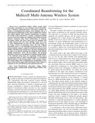
IEEE TRANSACTIONS ON CIRCUITS AND SYSTEMS—II: ANALOG AND DIGITAL SIGNAL PROCESSING, VOL. 46, NO. 2, FEBRUARY 1999 101 

Distortion Analysis of MOS Track-and-Hold 

Sampling Mixers Using Time-Varying Volterra Series 

Wei Yu, Subhajit Sen, and Bosco H. Leung, Senior Member, IEEE 

Abstract—A time-varying theory of Volterra series is developed 

and applied in the sampled-data domain to solve for harmonic 

and intermodulation distortion of a MOS-based track-and-hold 

sampling mixer with a nonzero fall-time LO waveform. Distortion 

due to sampling error is also calculated. These results, when 

combined with the continuous-time solution, quantify harmonic 

and intermodulation distortion of a track-and-hold type mixer 

completely. Closed-form solutions are obtained. As a practical 

consequence, it is shown that for certain fall-time, the distortion 

of track-and-hold mixers can be better than what would be 

predicted by a simple application of time-invariant Volterra series 

theory. 

Index Terms— Harmonic distortion, intermodulation distortion, 

intermediate frequency (IF), radio frequency (RF), timevarying 

Volterra series, track-and-hold sampling mixer. 

I. INTRODUCTION 

INCREASING demand for digital wireless personal communication 

devices, and steady improvements in the MOS 

device performance of scaled VLSI technologies, have allowed 

the feasibility of performing A/D conversion on radiofrequency 

(RF) signals directly or on their mixed down (IF) 

versions [1], [2]. Early A/D conversion of the received signal 

in a receiver chain pushes front-end signal processing 

functions such as channel-selection filtering and automatic 

gain control (AGC) into the digital domain, and thus helps 

to improve tolerance against process variations inherent in 

analog dominated front-end architectures and therefore the 

overall performance of the receiver. The key element crucial 

for good distortion performance of an A/D converter that 

digitizes RF signals is the track-and-hold circuit at the input 

of the A/D converter. This is because unlike a conventional 

baseband A/D converter, the track-and-hold circuit in an RF 

A/D application is inherently a mixer that mixes the RF signal 

down to baseband or a lower IF frequency in the process 

Manuscript received March 23, 1997; revised November 14, 1998. This 

work was supported by the Department of Electrical and Computer Engineering, 

University of Waterloo, and by the National Science and Engineering 

Research Council (NSERC) of Canada. This paper was recommended by 

Associate Editor Y. Inoue. 

W. Yu was with the Department of Electrical and Computer Engineering, 

University of Waterloo, Waterloo, Ont., N2L 3G1, Canada. He is now with 

the Information Systems Laboratory, Department of Electrical Engineering, 

Stanford University, Stanford, CA 94305 USA (e-mail: weiyu@stanford.edu). 

S. Sen was with the Department of Electrical and Computer Engineering, 

University of Waterloo, Waterloo, Ont., N2L 3G1, Canada. He is now with 

Arcus Technology Limited in Bangalore, India (e-mail: sen@arcustech.com). 

B. H. Leung is with the Department of Electrical and Computer Engineering, 

University of Waterloo, Waterloo, Ont., N2L 3G1, Canada (e-mail: 

bleung@sun14.vlsi.uwaterloo.ca). 

Publisher Item Identifier S 1057-7130(99)01746-2. 

of continuous-time to discrete-time conversion. Compared to 

the conversion of a band-limited signal in a conventional 

Nyquist-rate A/D converter, the mixing down process in a 

narrow-band VHF or UHF signal is much more nonlinear 

with nonlinear products increasing with input RF frequency. 

Linearity is crucial because the presence of adjacent channel 

interfering signals at the input generates spurious components 

in the desired channel band. The track-and-hold mixer also 

differs from a conventional mixer (such as a Gilbert multiplier) 

in that the frequency of the sampling clock (which serves as 

the equivalent of a local oscillator) may be a submultiple of 

the local oscillator (LO) frequency in a conventional mixer. 

In a subsampling track-and-hold mixer, the th harmonic 

of a sampling-clock with fundamental frequency may be 

mixed down with a carrier-tone at frequency to generate a 

baseband tone at frequency ( ). 

In this paper, the harmonic and intermodulation distortion 

of MOS track-and-hold mixers is thoroughly analyzed and 

related with simulation results. It is shown that a complete 

picture of distortion can be obtained by applying Volterra 

series analysis, hitherto applied only to continuous-time timeinvariant 

nonlinear systems, to time-varying circuits that are 

observed every clock period in the discrete-time domain such 

as in the case of a track-and-hold circuits in A/D converters. 

We have done this by developing a theory of Volterra analysis 

for time-varying systems valid under the assumption that the 

time-constant of the circuit is much smaller than the sample 

clock period. We have demonstrated that the incorporation 

of the time-varying analysis to Volterra series is essential for 

an accurate estimation of distortion for arbitrary fall-time in 

the sampling clock waveform. The closed-form formulas we 

obtained are useful in providing physical insights to the circuit 

designer. Successful applications which used these formulas in 

designing the front-end sampling mixer have been reported, for 

example, in an 150-MHz 13-bit 12-mW A/D converter in [3], 

and in a 400-MHz 12-bit 18-mW A/D converter in [4]. 

The rest of the paper is organized as follows. Section II 

explains the basic operation of the track-and-hold circuit as a 

mixer under the assumption of zero fall-time LO waveform. 

Expressions for harmonic distortion (HD and HD ) and 

intermodulation (IM and IM ) are derived using Volterra 

Series. The difficulty of extending this result to an arbitrary 

gate waveform is explained. Section III develops the 

theory of time-varying Volterra Series and shows that it is 

possible to extend the theory to time-varying systems by 

assuming that the output is observed in the sampled-date 

domain. Expressions for time-varying distortion are derived 

1057–7130/99$10.00 © 1999 IEEE

102 IEEE TRANSACTIONS ON CIRCUITS AND SYSTEMS—II: ANALOG AND DIGITAL SIGNAL PROCESSING, VOL. 46, NO. 2, FEBRUARY 1999 

Fig. 1. 

A track-and-hold mixer. 

Fig. 2. 

Mixing distortion using two tones. 

for the case of a simple track-and-hold mixer. In Section IV, 

sampling distortion is analyzed and expressions for harmonic 

and intermodulation distortion are derived. Section V describes 

SPICE simulation results for the simple track-and-hold mixer. 

These results are then explained using the theoretical results 

on the continuous-time, time-varying, and sampling distortion. 

Section VI analyzes the practical scheme of bottom-plate 

sampling using the theory developed. Conclusions are drawn 

in Section VII. 

II. TRACK-AND-HOLD SAMPLING MIXER 

A. Mixer Operation 

A single switch track-and-hold sampling mixer consists of 

a MOS transistor followed by a sampling capacitor (Fig. 1). 

The input is at RF or IF frequency. As applied at the 

gate goes high, the output tracks the input; as goes 

low, the output is sampled and held on the capacitor. The 

output is considered in the sampled-data domain. 

Before analyzing distortion, let us first define the terminology 

used in this paper. Suppose that a single pure sinusoidal 

input is applied at the input of the circuit, in this 

case to , we define the harmonic distortion of th order 

to be the magnitude of the term at the output .If 

two tones are applied at the input, frequencies at the sum and 

difference of input frequencies are present at the output. So, 

two different kinds of second order intermodulation (IM ) are 

possible. For an input of ,IM is defined as 

the magnitude of 

term at the output, and IM 

that of 

term. Likewise, intermodulation of third 

order (or IM ) is defined as the magnitude of 

term when an input of 

is applied. The 

physical origin of HD and IM is the same, and HD is 

related to IM by a factor of 2. So, we are more interested 

in IM than IM . In the following analysis, unless explicitly 

specified, IM refers to IM . 

For example, in the case that the RF input contains two tones 

at frequencies (say at 100.3 MHz) and (say at 100.4 

MHz), respectively, with a sampling clock frequency at 

100 MHz. The components visible in the baseband are shown 

in Fig. 2. The 100-kHz component is the IM component 

at . The 200-kHz component is due to IM at 

(200.2 MHz) mixed down to baseband. The 

component at 700 kHz is the IM component at 

(200.7 MHz) mixed down. We also observe HD components 

at 600 and 800 kHz as well as HD component at 900 

kHz. We may note that by using a differential architecture, 

the even order distortion (e.g., HD , IM ) may be made 

considerably smaller (by the mismatch factor) than in a singleended 

architecture. 

A rigorous distortion analysis of the simple track-andhold 

circuit with arbitrary input frequency and arbitrary LO 

waveform is difficult for the following reasons. 

• The relation between drain current and terminal voltages 

is nonlinear. 

• The body effect and bias-dependent junction capacitors 

produce additional nonlinearities. 

• The circuit is time varying due to the modulation of drainsource 

conductance by the applied gate LO waveform. 

• The precise instant of sampling depends not only on 

the LO waveform but also on the input amplitude and 

frequency resulting in sampling distortion. 

Previous work on track-and-hold distortion focused on its 

application in baseband A/D converters [5], [6]. These have 

mainly tackled the distortion problem of a CMOS switch 

by isolating the distortion into the “tracking error” and the 

“aperture error” components with low-frequency single-tone 

inputs. They used assumptions that are not valid for trackand-hold 

mixers applications, the most important of which is 

the circuit time-invariant assumption. In [7], track-and-hold 

type mixers for continuous-time output using Volterra Series 

approach were analyzed. Again, the analysis did not take into 

account the sampling and the time-varying nature of the circuit 

due to periodic but arbitrary gate LO waveforms. 

In the following, we propose to analyze distortion using 

time-varying Volterra series. To simplify the problem, we 

will abstract the most essential features of MOS track-andhold 

distortion by excluding the nonlinear bias-dependent 

components of junction capacitors and body effect from the 

MOS transistor model. Further analysis incorporating these 

second order effects results in a slight modification of only a 

few decibels. As a first step, we will solve for mixer distortion 

in the continuous-time mode, which corresponds to the case 

where LO waveform has a sharp cutoff. This also serves

YU et al.: DISTORTION ANALYSIS OF MOS TRACK-AND-HOLD SAMPLING MIXERS 103 

ON. (This is true even for high-frequency RF if a subsampling 

technique is used with a sufficient subsampling factor.) Under 

this condition, the distortion components seen in the discretetime 

frequency domain are the same as that for the case 

when the track-and-hold is working in the continuous-time 

mode with the gate voltage at and the MOS transistor 

stays ON. Therefore, to calculate distortion components for 

the ideal sampling case, we only need to analyze distortion 

for the continuous-time mode, which can be done using the 

time-invariant Volterra series theory. 

Fig. 3. 

Mixing using ideal sampling. 

C. Volterra Series and Harmonic Distortion 

Under some general continuity conditions, a time-invariant 

system may be expanded into the sum of a linear term, a 

second-order term, and a third-order term, etc. [8]. Mathematically, 

if the input is , the output is represented by 

a series of the type, 

to illustrate the essential steps in applying Volterra series in 

distortion analysis. 

B. Mixer Using Ideal Sampling 

The mixer operation under ideal sampling can be approximated 

by the following simplified model. We assume that 

a constant high voltage is applied at the gate, an RF signal 

at frequency is applied at the input, and that the output 

is sampled using an ideal sampling process. Since the circuit 

is nonlinear, we expect the input signal to be attenuated by 

the gain of the network along with harmonic components at 

where 2, 3, , as shown in Fig. 3(b). The ideal 

sampling process followed by an ideal low-pass filter with a 

cutoff frequency at /2 is then applied to the output. The 

effect is to replicate the output spectrum by shifting it by , 

where 1, 2, , so that a shifted component of output is 

mixed down to near DC. This is shown in Fig. 3(d). We note 

that harmonic components at now reappear near DC at 

and close to in the baseband. We may 

also note that it is possible to mix down the output to the same 

positions in the baseband by using a sampling clock with a 

frequency that is a subharmonic of (i.e., subsampling). The 

observation is that the harmonic distortion of the mixer without 

sampling [i.e., Fig. 3(b)] is the same as the harmonic distortion 

of the sampled signal in the baseband [i.e., Fig. 3(d)] if ideal 

sampling is assumed. Therefore, under the ideal sampling 

condition, harmonic distortion can be calculated as if sampling 

has not occurred, and the system is operating in the continuoustime 

mode. 

The mixing process with ideal sampling just described may 

now be used to approximate a track-and-hold circuit at whose 

gate an ideal square-wave is applied. When the gate voltage 

is at , the MOS transistor is in the triode region and the 

output tracks the input voltage. When the MOS turns OFF 

instantaneously, as in the case of an ideal square-wave gate 

voltage, the tracked output voltage is held onto the capacitor. 

Assuming that the time-constant of the circuit is much smaller 

than the gate ON period, the output voltage reaches a steadystate 

value within several time-constants after the MOS turns 

whose convergence is uniform. More succinctly, we write, 

(2) 

where represents the th order operator with kernel . 

This series is called the Volterra series. It can be shown that 

Volterra kernels form a basis for sufficiently well-behaved 

systems, i.e., a mildly nonlinear system can be expanded in 

a Volterra series in one and only one way. 

Expanding a system in Volterra series enables us to find 

its frequency response and hence its sinusoidal response, so 

Volterra series is directly related to harmonic distortion [9]. 

For example, the response to a sinusoidal input for a secondorder 

system contains a term at twice the input frequency and 

a term at DC. The magnitude of each term is related to the 

corresponding terms in the Volterra series. More specifically, 

for an input of 

, the output is 

The third-order term can be derived in a similar way. Following 

the definition for harmonic distortion, harmonic distortion 

is related to Volterra kernels in the following way: 

(1) 

HD (3) 

HD (4)


Similarly, intermodulation can be quantified as well: 

IM (5) 

IM (6) 

Therefore, obtaining the Volterra series coefficients is the key 

in calculating harmonic distortion and intermodulation. 

D. MOS Mixer Volterra Coefficients 

We now analyze harmonic distortion of an ideal sampling 

mixer using the continuous-time model by calculating its 

Volterra coefficients. First, it can be shown by a Volterra 

analysis that at sufficiently low frequencies the distortion 

is mainly determined by the nonlinear source-to-drain – 

characteristic of the MOS transistor and that distortion due to 

bias-dependent junction capacitance is quite small for typical 

values of MOS model parameters. We also choose to ignore 

body effect for simplicity in analysis, but note that this choice 

modifies neither our method of distortion analysis nor the 

significant conclusions regarding distortion in MOS trackand-hold 

mixers. Further, the only parasitic capacitance of 

importance is the junction capacitance at the output side whose 

effect is to increase the value of the sampling capacitor. 

Therefore, in deriving the Volterra series coefficient, we can 

assume the configuration in Fig. 1 and use the most basic MOS 

equation 

where , and is the threshold voltage. Either 

the input or the output side may be regarded as source. The 

system differential equation thus becomes 

(7) 

(8) 

The solutions to this set of differential equations are the 

Volterra coefficients , , and . Since we assume a 

constant gate voltage, hence a constant , we can show that 

(10) 

(11) 

(12) 

where the assumption of small time-constant ( )is 

used, and also the expressions are symmetrized. Substituting 

(10)–(12) into (3)–(6) yields the harmonic distortion and 

intermodulation 

HD (13) 

HD (14) 

IM (15) 

IM (16) 

It must be emphasized that the above analysis assumes a 

constant gate voltage. This applies to the case of perfect square 

LO sampling if the system time-constant is much smaller than 

the sampling period. However, if the sampling-clock voltage 

deviates from the ideal square wave, two effects start to emerge 

which will invalidate the continuous-time model. If the gate 

voltage falling edge is not instantaneous, the approximate 

time-constant of the circuit, as given by 

where . Express in its Volterra series 

where , substitute the expansion into (8), 

and keep only the first three order terms, so we get 

Note, is first order since the input is a pure sinusoidal; 

the term is second order; and is third order. Now, 

equating the coefficients, we have 

gradually increases since the MOS ON resistance increases as 

the MOS leaves the triode region. In addition, the precise 

instant of sampling depends not only on the gate falling 

edge slew-rate waveform but also on the input amplitude and 

frequency, which results in sampling distortion. This leads to 

a situation where the final sampled voltage on the sampling 

capacitor when the MOS transistor turns OFF deviates from 

the steady-state voltage on the capacitor predicted by Volterra 

series theory when the MOS transistor is ON. Therefore, the 

sampled voltage can no longer be predicted with a timeinvariant 

theory. This leads us to develop the theory of the 

time-varying Volterra Series. 

(9) 

III. TIME-VARYING VOLTERRA SERIES 

As mentioned in the previous section, it is necessary to 

generalize the Volterra series to time-varying systems in order 

to analyze the track-and-hold mixer with an arbitrary LO 

waveform. In this section, we develop a time-varying Volterra


series, explore its frequency response, and show that the timevarying 

Volterra series can be applied in the sampled-data 

domain to solve for time-varying distortion exactly. 

A. Time-Varying Systems 

The notion of impulse response can be generalized to timevarying 

systems by adding another time variable [10]. The 

impulse response of a linear time-varying system, ,is 

a function of two time variables, where is the observation 

time and the launch time. represents the output 

observed at time for an impulse input launched at time . 

The system response for an arbitrary input can be found from 

using the following: 

(17) 

Under general continuity conditions, a linear time-varying 

system is completely characterized by its two-dimensional 

impulse response, otherwise known as the kernel. 

Higher order kernels are generalized in a similar way. For 

example, a second order kernel has two launch time variables 

and an observation time variable. 

is the system 

response to two impulses launched at time instants and . 

In general, a mildly nonlinear time-varying system has the 

following Volterra series expansion: 

Fig. 4. 

Composition of second-order system from first-order systems. 

If we set 

in the above, we obtain the impulse 

response of the first-order time-varying system 

if 

if . 

(20) 

We would also like to calculate the second-order kernel. In 

general, a second-order system can be thought of as the 

composition of linear systems as shown in Fig. 4. Suppose 

that the impulse responses of the linear systems are , 

, and , respectively, the second-order kernel 

can be computed as follows: 

(21) 

The expression for third order systems is similar. If in Fig. 4, 

is second order, and therefore the overall system is third 

order, the overall system kernel is then 

(18) 

Recall that in the linear time-invariant case, the impulse 

response may be found in either time domain or frequency 

domain. The frequency domain solution is often much easier 

to obtain than the time domain impulse response. However, 

for time-varying systems, frequency response is no longer 

well defined and, hence, it is necessary to directly apply 

time domain impulses at the system input to find the output 

expression. This amounts to solving the differential equation 

directly, which is not trivial in general. However, for firstorder 

differential equations such as the track-and-hold mixer 

equation, this method is feasible. 

Consider the mixer equation (9), where is time varying. 

The zero state response of the first-order equation 

can be obtained using an integrating factor 

(19) 

(22) 

Therefore, as was done for the time-invariant case, and 

can be solved consecutively. For example, the second-order 

kernel is found by substituting from (19) and setting 

input as an impulse in the solution to the second-order equation 

in (9) 

(23) 

Since the differential equations are linear and first order, there 

is no theoretical difficulty in obtaining the solution. Following 

this method, the complete time domain solution to the system 

can be obtained. 

Now, in a track-and-hold mixer where the output points of 

interest are at the sampled points, we need to sample and 

apply Fourier analysis to the sampled points to obtain the second 

order distortion. This procedure, although straightforward 

in theory, is tedious even for a simple system such as the trackand-hold 

mixer. However, as will be shown in the next section, 

by exploring the frequency domain interpretation and by taking 

advantage of the fact that output is in the sampled-data domain, 

the problem can be simplified significantly. 

B. Sampling Process 

Let sampling occur at time 0, let be the timevarying 

kernel of the system with a nonzero fall-time LO


waveform, the linear term in the sampled output voltage is 

ZIR (24) 

where is the sampling period, and ZIR is the zero input 

response due to the initial condition. Since we have assumed 

that the RC time-constant for the track-and-hold mixer is much 

smaller than the sampling period, ZIR is negligible. Also 

because of the small time-constant, we may replace the lower 

limit of integration by 

(25) 

Further, since the output voltage of interest is at the sampling 

instant, the time-varying characteristic of importance occurs 

during the time within a few time-constants before the sampling 

instant. This means that the same Volterra kernel applies 

to every sampling instant, except the kernels are shifted by 

, integer multiples of the sampling period. To simplify 

computation, we want to keep the Volterra kernel identical 

for each sampling period. Therefore, instead of shifting the 

kernel, we shift the input signal backward in time by and 

keep the sampling instant at time 0. This effectively keeps 

the functional form of the kernel identical for all samples. 

Further, there is nothing special about sampling points . 

So, if sampling occurs at an arbitrary time , the sampled 

voltage can be represented as 

(26) 

This is a fictitious signal, whose value at represents 

the sampled value of the output if sampling is to occur at .If 

sampling occurs at instants , the output voltage samples are 

just , , , . Hence, the nonideal sampling 

of the output signal is reduced to the ideal sampling of 

, where is related to the input by (26). Now, 

because the harmonic distortion of the ideal sampled 

is the same as the harmonic distortion of the continuous 

signal , the problem of calculating distortion in nonideal 

sampled output is reduced to the problem of calculating the 

distortion in the continuous signal . The transformation 

from (24)–(26) also reduces a time-varying system to a timeinvariant 

system, as the relation between and in (26) is 

time invariant. This situation is analogous to the analysis of 

discrete control systems where, although a zero-order-hold is 

not a time-invariant operation in the continuous-time domain, 

the input–output relation is nevertheless time invariant in the 

sampled-data domain. 

It remains to find the impulse response of the linear timeinvariant 

system (26). Denote the impulse response in time 

and frequency domain by and , respectively. To 

find , set in (26), it follows that 

if 

(27) 

if . 

The frequency response is its Fourier transform 

(28) 

where, again, is the time-varying kernel. 

The same technique applies to higher order systems. For a 

second-order system, the sampled-data domain response is 

and the frequency response is 

(29) 

(30) 

Again, the second-order kernel may be obtained from its 

composition from first-order systems as in (21). 

The frequency domain expression is of the most interest. 

It is in fact possible to bypass the time domain expression 

and obtain frequency domain result directly. Assuming the 

composition form as in Fig. 4, substituting (21) into (30), then 

More succinctly, and for convenience only, define 

and 

we arrive at the formula 

(31) 

(32) 

(33) 

In particular, setting gives the sampled frequency 

domain kernel for the system of Fig. 4 

(34) 

The third-order frequency domain representation is similarly 

derived. If in Fig. 4 is second order, then 

and the overall frequency domain kernel is 

(35) 

(36) 

C. Time-Varying Mixer 

We now analyze the track-and-hold mixer of Fig. 1 in the 

sampled-data domain. Assume the input side is source, the


output drain, 1 from the basic MOS equation, we have 

We define MOS conductance as 

. The MOS 

enters the cutoff region at 

, so the value of 

goes to zero at each sampling point. Now, since we have 

assumed that the RC time-constant is small, the region of 

most importance is the time right before the sampling instant. 

Therefore, we can approximate by a linear function prior 

to each sampling point. This assumption is most valid if the 

system time-constant is smaller than the fall-time of the gate 

voltage. In practical cases where this is not true, the analysis 

yields a limiting case and provides a useful bound. Now, the 

slope of the linearly varying is just the slope of the cutting 

edge minus the slope of the input signal to a first-order 

approximation. So, if we define 

, where 

and are as indicated in Fig. 1, and define , the 

MOS equation becomes 

The second-order term is evaluated using (33), where the 

time-varying kernel is obtained from its composition from 

first-order terms. Mechanically, is substituted by , and 

is substituted by 

Again, approximate 

(38) to (40) 

(40) 

by its Taylor expansion, substitute 

erf 

Let , , expand into its Volterra series as 

before, and collect the first three order terms, we have 

Fortunately, at 

numerically 

erf 

(41) 

, the last two integrals may be evaluated 

(42) 

To calculate , we use (31) where the time domain 

is as found in (20). 

(37) 

where 

comes from the evaluation of definite 

integrals. (The relative contributions from the two integrals are 

comparable.) Finally, is also obtained by its composition 

from first- and second-order systems 

where the substitution of and are made. 

This integral cannot be evaluated analytically. However, we 

are interested in the value of the integral when is close to 0, 

so the upper limit of the integral is close to zero. The integrand 

is a rapidly increasing function of as approaches 0; so, 

effectively, the only relevant portion of the integration is when 

is close to 0. Therefore, we can assume that . 

In this case, the integral becomes: 2 erf (38) 

(43) 

We need to evaluate the above expression for . Because 

each term contains two integrals, there is a total of 

four definite integrals. By substituting the expression for 

from (38), and from (41), we can evaluate the integral 

numerically 

(44) 

where 

. Equations (39), (42), and (44) are the 

final solution to the sampled time-varying Volterra series. To 

summarize the results in terms of circuit parameters 

So, setting 

gives 

(45) 

(39) 

1 Assuming the output side being source will give a slightly different 

differential equation, but the form of the answer is the same. 

2 The error function is defined as erf(t)=(2=p) 

t 

0 e0x dx. 

(46) 

(47)


where again , , numerically. 

Recall that this result is obtained by assuming a linearly 

decreasing . In reality, is nearly constant for a large part of 

the sampling period. Therefore, this solution is an asymptotic 

case. 

Comparing the Volterra coefficients for the nonideal sampling 

MOS track-and-hold mixer with the ideal sampling 

case, at low frequency we find that nonlinearity due to the 

time-varying nature is much smaller than the ideal sampling 

case. However, time-varying distortion varies with the cube of 

input frequency; so, theoretically, at high enough frequency, 

the time-varying distortion will overtake the continuous-time 

distortion. This happens at an RF frequency around 2–3 

GHz. The fact that time-varying distortion is small at low 

frequency can be intuitively explained. There are two sources 

of nonlinearity from the MOS governing equation 

Fig. 5. 

Sampling error. 

, and solve for the cutoff time 

An obvious source of nonlinearity is the square term , 

but this effect is secondary for the ideal sampling case, where 

the major contributing factor is the input signal dependent 

conductance 

. However, in a nonideal sampling 

mixer, the first-order signal dependence in is eliminated 

because sampling always occurs when 

, hence the 

local behavior of prior to cutoff is approximately same for 

each sampling point. Then, the only nonlinear factors left are 

the signal dependence in the derivative of the conductance and 

the term, which are significantly smaller. However, we 

are not getting something for free here. Although in the case 

of a nonideally sampled mixer, the 

term causes 

much less input dependence in , the term manifests as an 

altogether different source of distortion. Because cutoff occurs 

when 

, the cut-off time is now input signal 

dependent. In other words, the distortion in the amplitude 

domain is shifted to the time domain by nonideal sampling. 

The signal dependent cutoff time is called sampling error, 

which will be discussed in detail in the next section. 

IV. SAMPLING ERROR 

In the development of time-varying distortion analysis in 

sampled-data domain, the output voltage is assumed to be 

sampled at equally spaced instants. This assumption is not 

true if the gate voltage has a nonzero fall-time. The instance of 

sampling is when 

, so the time at which sampling 

occurs depends not only on gate voltage but also on the 

input voltage. The signal-dependent sampling time introduces 

additional distortion term, which can again be quantified using 

Volterra series. 

Suppose the input signal is smooth—call it —and we 

intend to sample the input at time 0. Let the gate voltage have 

a finite-slope falling edge with slope , where 

as shown in Fig. 5, i.e., the falling edge has the form 

. Since the MOS enters cutoff at , and 

the input is applied at the source side, sampling occurs at the 

instant when 

. Now, use the approximation 

(48) 

where we assumed that is large. Substitute the above 

expression for into the Taylor expansion for around 

0, and collect the first three order terms, we have 

(49) 

where again the assumption of large is used. So, due 

to the finite fall-time, the sampled value differs from 

the desired value by additional signal-dependent terms, 

which produce distortion. Since the sampling time is arbitrary, 

(49) is valid if time 0 is replaced by an arbitrary sampling time. 

The signal dependence can be analyzed by Volterra series. 

The linear term in (49) is ,so . The secondorder 

term is the product of derivative with the function 

itself, and its Volterra series coefficient can be found using 

the composition rule (21) followed by symmetrization. The 

second order coefficient is found to be 

and for the third-order, 

(50) 

(51) 

Using these expressions in (3)–(6), harmonic distortion and 

intermodulation can be calculated exactly 

HD (52) 

HD (53) 

IM (54) 

IM (55)


Comparing the sampling distortion as given by (52)–(55) to 

the continuous-time distortion as given by (13)–(16), we can 

show that the sampling distortion becomes comparable to the 

continuous-time distortion when the fall-time is in the order 

of , where is the RC time-constant formed by the MOS 

resistor and the load capacitor, and is the period of the input 

signal. Therefore, sampling error becomes a bigger problem at 

high frequency, where has to be small. 

V. SIMULATION RESULTS AND COMPARISON TO THEORY 

SPICE simulations are performed to verify the theoretical 

results derived in the previous sections for the cases of 

continuous-time, time-varying, and sampling distortion. The 

three factors have to be combined in order to fully explain the 

distortion of a track-and-hold mixer whose gate voltage has a 

finite falling slope. 

Although RF is normally carried in the 900-MHz range, 

we start off the simulation at 100 MHz assuming the mixer is 

used in a first-stage IF digitizer application. The track-and-hold 

mixer is fed with either a single tone or two tones near 100 

MHz at its IF input. For example, to estimate intermodulation 

distortion, two tones at 100.3 and 100.4 MHz are applied at 

the IF input, and a 100-MHz square-wave sampling clock is 

applied at the gate. Consistent with our standing assumptions, 

the RC time-constant during ON period has been chosen to 

be approximately 20 ps, and therefore much smaller than the 

5ns ON period of the sampling clock. Finally, we note that 

the results presented in this section are applicable in the RF 

frequency range as well. 

A. Simulation Accuracy and Speedup 

A number of precautions have to be taken to ensure numerical 

accuracy, convergence, and charge conservation in 

the simulations. The simulation accuracy has to be calibrated 

with ideal sine tones and simple linear models. The maximum 

time-step value and time-step update algorithm also have to 

be chosen consistent with the dynamic range to be expected 

from simulations. The time-step parameter (delmax) is crucial 

in determining simulation accuracy. Our experience shows 

that a delmax as low as 0.1 ps is necessary to achieve 

reasonably accurate results. Charge conservation is particularly 

difficult to achieve. It depends on the level of the MOS model 

chosen, the MOS device capacitance (capop) model, and the 

integration method. Our experience has been that the charge 

conservation models (capop 4 and capop 9 in HSPICE) 

either have poor convergence properties or produce numerical 

inaccuracy. We have bypassed the charge-injection and chargeconservation 

problems by calculating the device capacitances 

separately and inserting linear capacitances into the circuit and 

using a no-capacitance (capop 5) model. Without these 

precautions, the simulation results can be rendered totally 

useless. 

SPICE simulation for very small values of delmax can 

make the simulation time impractically long. A major factor in 

speeding up simulation has been the insight that the RC timeconstant 

during the ON period of the MOS transistor is much 

smaller than the ON period. Thus, since the circuit reaches 

steady state within only a tiny fraction of the period, we may 

Fig. 6. Harmonic distortion (HD 2 and HD 3 ) of a track-and-hold mixer 

versus fall-time at 100 MHz (body effect excluded). 

only need to simulate around the sampling edge. This has 

been accomplished by repeated simulations at uniform phase 

intervals of the input sine-wave for a total phase interval of 

360 , which corresponds to exactly one period of the mixed 

down frequency. 

B. Harmonic Distortion 

Fig. 6 plots the second- and third-order harmonic distortion 

of a track-and-hold mixer with a MOS switch of 102 

m/0.8 m. The sampling capacitance is 0.2 pF. An additional 

capacitance of 0.152 pF is added to account for source/drain 

capacitance. A square-wave with fall-time varying between 10 

ps and 1.28 ns is applied at the gate. In this simulation, the 

SPICE model parameter gamma has been set to 0 to exclude 

substrate bias modulation of the threshold voltage. The HD 

curve can clearly be divided into three regions: 

1) a relatively flat portion corresponding to small fall-times 

up to a few tens of picoseconds; 

2) a region with distortion decreasing with fall-time and 

having a distinct minimum; and 

3) a region with distortion increasing with fall-time occurring 

for large fall-times and with a distinct slope of 20 

dB/decade for HD and 40 dB/decade for HD . 

Region 1 shows an asymptotic behavior toward 0 falltime. 

This asymptotic distortion value agrees with the prediction 

from continuous-time (time-invariant) harmonic distortion 

model (13)–(16). This is to be expected since we have shown 

in Section II that for fall-time of 0, the harmonic distortion of 

the MOS track-and-hold distortion approaches the continuoustime 

harmonic distortion. 

Region 3 displays asymptotic behavior toward a log-linear 

relation that increases at 20 dB/decade for HD and 40 

dB/decade for HD . This line agrees exactly with the distortion 

predicted by sampling error (52)–(55). Hence, for large falltimes, 

harmonic distortion is limited by sampling distortion. 

Region 2 can be explained by time-varying distortion of a 

MOS track-and-hold mixer at whose gate a nonzero fall-time 

sampling signal is applied. In Section III, it was pointed out


Fig. 7. Effect of input frequency on harmonic distortion HD 3 (body effect 

included). 

that for the case of nonideal sampling, if sampling error is 

neglected, harmonic distortion, now attributed to time-varying 

distortion, becomes very small. This is responsible for the 

dip in distortion curve in region 2 since in this intermediate 

region the fall-time is large enough so that contribution due 

to the continuous-time operation is small, while at the same 

time the fall-time is small enough that sampling distortion 

does not manifest itself. Overall, the simulation result shows 

quantitative agreement with the theory in regions 1 and 3, and 

qualitative agreement in region 2. 

In order to highlight the role of time-varying distortion, we 

note that the third order sampling distortion is proportional 

to the square of the input frequency . Thus, for large 

fall-times, by reducing the input frequency we may be 

able to reduce sampling distortion sufficiently enough for 

time-varying distortion to manifest itself over a wider 

window (i.e., region 2) of the sweep of fall-time. Conversely, 

by increasing the input frequency, sampling-distortion may 

increase to the point that it completely swamps out the 

time-varying distortion. This trend is confirmed in Fig. 7 

which plots HD versus fall-time for 25, 100, and 500 MHz. 

Body effect is included in these simulations. 

Thus, we have shown both by simulation and by 

time-varying analysis that a region with a distortion 

smaller than the 0 fall-time asymptotic value predicted 

by continuous-time distortion exists, which explains the 

decreasing distortion and the minimum observed in this 

region. The practical significance of this result is that the 

distortion of a MOS track-and-hold mixer can actually 

be better than what would be predicted by time-invariant 

continuous-time Volterra series theory by a proper choice of 

fall-time. Note that this does not occur for HD and IM in 

this particular case because sampling distortion is bigger than 

the continuous-time distortion even for small fall-times. 

C. Intermodulation Distortion 

Fig. 8 shows the intermodulation distortion of the MOS 

track-and-hold mixer obtained by applying two tones at 100.3 

Fig. 8. Intermodulation (IM + 2 and IM 3) of a track-and-hold mixer versus 

fall-time at 100 MHz. 

and 100.4 MHz at the IF input and a 100-MHz sampling clock 

at the gate. IM resulting from the difference of the two 

input frequencies is very small. IM , which behaves in the 

same trend as HD , is shown. The distortion characteristics 

again match very well with theoretical predictions both for 

continuous-time formulas developed in Section II and for 

the sampling error distortion developed in Section IV. The 

initial decrease in IM curve as the fall-time increases may 

be explained by the system time-varying nature. In general, 

intermodulation distortion is slightly worse than harmonic 

distortion, and they exhibit similar behavior with respect to 

fall-time. 

VI. BOTTOM-PLATE SAMPLING 

In this last section, we solve for distortion in the bottomplate 

sampling scheme as a practical application of the theory 

developed. The bottom-plate sampling scheme is shown in 

Fig. 9. The input is at , and the output is taken as the 

differential voltage between and . During sampling, 

the bottom transistor opens first, which effectively fixes the 

amount of charge on the sampling capacitor . Then, the top 

transistor opens, which fixes the voltage levels of and . 

In the figure, is included as the junction capacitor of the 

top switch, which can be fairly large, and is included as 

the junction capacitor of the bottom switch, which is typically 

much smaller. 

The main advantage of bottom-plate sampling is that it 

eliminates the charge injection problem. When a MOS transistor 

turns OFF, the charges that comprise the inversion layer 

are injected to either the source or the drain side. Which 

side the charges go to depends on the relative impedance. 

In the track-and-hold mixer of Fig. 1, the impedance on the 

output side ( ) is small, so it attracts the extra charges, 

which disturb the output signal level. This does not happen in 

bottom-plate sampling. At the opening of the bottom transistor, 

charges are injected to the ground, while at the opening of the 

top plate, the charges are injected back to the input. In either 

case, little extra charges are dumped to the sampling capacitor.


Fig. 10. 

Simplified bottom plate sampling. 

Fig. 9. 

Bottom plate sampling. 

To analyze this circuit, we first model the transistors as 

simple switches. It is easy to show that the output voltage can 

be expressed as 

(56) 

where and are the voltages at node when 

the bottom switch and top switch each opens, respectively. 

The total distortion in the output is, therefore, the sum of two 

factors, one due to the opening of the bottom switch, and 

the other due to the opening of the top switch. Distortions 

due to the two parts should be analyzed separately. Each part 

would consist of three factors: the continuous distortion, the 

time-varying distortion, and the sampling distortion. 

A. Distortion in Opening Bottom Switch 

We first notice that the sampling error is small in opening 

the bottom switch. This is because the source and the drain of 

the bottom switch are kept at a constant voltage at the ground 

level. This eliminates signal-dependent sampling. 

Next, the continuous-time distortion can be calculated from 

the coupled differential equations. Assume that both transistors 

are in the triode region with device constants and , 

respectively. Define 


. The governing equations are 

(57) 

where and are the voltages on the nodes and .We 

assume the Volterra series expansions 

(58) 

If we assume that and , the output 

of interest, is close to the case without the bottom 

transistor. This is not unexpected because ’s are almost 

independent of , and is much larger than . So, 

in this case is the same as in the case without the bottom 

switch, as given by (14)–(16). In particular, 

HD (59) 

IM (60) 

Note that the continuous-time distortion is determined by the 

ratio of the top transistor. 

Finally, we need to take the time-varying distortion into account. 

The difficulty is that we have a second-order differential 

equation with nonconstant coefficients for which solutions are 

not easily found. However, the situation may be simplified. 

When the bottom switch opens, the resistance between the 

source and the drain increases with time and eventually reaches 

infinite; but the top switch stays closed, hence its resistance is 

relatively small. So we can neglect the top switch altogether 

and simplify the problem to that in Fig. 10. With only one 

capacitive node, this circuit is modeled by a first order equation 

which we can solve. 

We are ultimately interested in the differential voltage 

( – ). But since node is purely sinusoidal, the distortion in 

( – ) is same as the distortion in . Let be the voltage in 

node . The differential equation for the system is as follows: 

(61) 

where again , and . 

Using the methodology developed in Section IV, timevarying 

distortion may now be derived. Note here we have 

at the right side of the first-order equation, which must 

be kept as an operator in the derivation, i.e., 


(62)


After carrying out the necessary computation, the final expressions 

for time-varying distortion turn out to be 

(63) 

(64) 

(65) 

where is related to fall-time as defined before, and 

, , numerically. Again, these 

distortion components are small. 

Therefore, as the bottom switch opens, for a small falltime, 

distortion is bounded by distortion produced by the 

continuous-time operation as expressed in (59) and (60). Since 

both the time-varying and the sampling distortion are small, 

distortion due to bottom switch is small at large fall-times. 

B. Distortion in Opening Top Switch 

The distortion analysis for the top switch is considerably 

simpler. This is because when the bottom switch is open, 

the circuit is identical to the case in Fig. 1, except that the 

capacitor is primarily due to parasitics. The distortion again 

consists of three parts: continuous-time, time-varying, and 

sampling distortion. 

The continuous-time distortion is given by (13)–(16) 

where the capacitor 

HD (66) 

IM (67) 

is 

(68) 

Since the capacitor in this case is primarily due to the parasitic 

which is much smaller than in the single switch case, the 

continuous-time distortion is small. The sampling distortion 

is the same as before, as given by (52)–(55) 

HD (69) 

IM (70) 

Again, the time-varying distortion is very small. 

Therefore, as the top switch opens, because both continuoustime 

and time-varying distortion are small, the total distortion 

is mainly due to sampling error, which is significant at large 

fall-times. 

C. Total Distortion 

We see that distortion due to the opening of the bottom 

switch comes from continuous-time operation, and that due to 

the opening of the top switch comes from sampling, so the 

total distortion is a linear combination of the two as in (56). 

HD 

IM 

(71) 

(72) 

Therefore, distortion for a bottom-plate sampler at small falltime 

is bounded by the continuous distortion, and distortion at 

large fall-time is bounded by sampling distortion. The major 

difference between this and the simple case of the track-andhold 

mixer is that the distortion due to sampling (when the top 

switch opens) is lessened by a factor of 

, which 

is significant. So, distortion due to nonzero fall-time is less a 

problem in bottom-plate sampling than in the simple case of 

Fig. 1. This is another advantage of bottom-plate sampling. 

VII. CONCLUSIONS 

The operation of a MOS track-and-hold circuit as a mixer 

is explained. It is shown that conventional nonlinear timeinvariant 

analysis using Volterra series, while useful for 

explaining the behavior of the circuit for ideal sampling 

clock waveform, fails to account for its behavior for nonzero 

fall-time of the sampling clock. The theory of time-varying 

Volterra series is developed and applied to the MOS trackand-hold 

circuit in sampled-data domain. Expressions for 

harmonic and intermodulation distortion for nonzero fall-time 

LO waveform are derived. Nonzero fall-time also introduces 

sampling distortion for which distortion formulas are derived. 

SPICE simulation on the track-and-hold sampling mixer is 

performed, and the results are successfully explained for all 

fall-times by combining the theories of continuous-time, timevarying, 

and sampling distortion. Finally, the practical scheme 

of bottom-plate sampling is analyzed. 

ACKNOWLEDGMENT 

The authors wish to thank an anonymous reviewer for 

correcting a numerical error in the derivation. 

REFERENCES 

[1] P. Y. Chen, A. Rofougaran, K. A. Ahmed, and A. A. Abidi, “A highly 

linear 1-GHz CMOS downconversion mixer,” in Proc. Euro. Solid-State 

Circuits Conf., Sevilla, Spain, 1993, pp. 226–227. 

[2] A. Hairapetian, “An 81-MHz IF receiver in CMOS,” IEEE J. Solid-State 

Circuits, vol. 31, pp. 1981–1986, Dec. 1996. 

[3] S. Sen and B. Leung, “A 150MHz, 13-bit 12.5mW IF digitizer using 

sampling mixer,” in Proc. IEEE Custom Integrated Circuits Conf., 1998, 

p. 233. 

[4] A. Namdar and B. Leung, “A 400MHz, 12-bit 18mW IF digitizer using 

mixer inside the sigma-delta modulator loop,” in Digest Int. Solid State 

Circuits Conf. (ISSCC), San Francisco, CA, 1999. 

[5] Y.-M. Lin, “Performance limitations on high-resolution video-rate 

analog-digital interfaces,” Ph.D. thesis, Univ. Calif., Berkeley, 1990. 

[6] D. Cline, private communication, 1995. 

[7] C. D. Keys, “Low-distortion mixers for RF communications,” Ph.D. 

thesis, Univ. Calif., Berkeley, 1994.


[8] M. Schtzen, The Volterra and Wiener Theories of Nonlinear Systems. 

New York: Wiley, 1980. 

[9] R. Meyer, “Advanced integrated circuits for communications,” Cal 

VIEW, 1995, UC Berkeley EECS 242 Course Notes. 

[10] C. D. Hull, “Analysis and optimization of monolithic RF downconversion 

receivers,” Ph.D. thesis, Univ. Calif., Berkeley, 1992. 

Wei Yu received the joint B.S. degree in computer 

engineering and mathematics from the University of 

Waterloo in 1997, and the M.S. degree in electrical 

engineering from Stanford University in 1998. He 

is currently a Ph.D. candidate in the information 

systems laboratory in the Electrical Engineering 

Department at Stanford University. His current research 

interest is in the transmission theory for 

digital communications. 

Bosco H. Leung (S’84–M’85–SM’92) received the 

Ph.D. degree from the University of California, 

Berkeley, in 1987, the M.Sc. degree from the California 

Institute of Technology in 1980, and the B.Sc. 

degree from the Rensselaer Polytechnic Institute in 

1979, all in electrical engineering. 

From 1980 to 1983, he was with Northern Telecom, 

Canada, working on analog circuit design. 

He is currently a Professor with the Electrical and 

Computer Engineering Department of the University 

of Waterloo, Canada. His main research interest is in 

CMOS and BiCMOS mixed analog/digital integrated circuits, in particular, on 

analog to digital converters. He has published more than 30 technical papers 

and has received patents in this area. He has recently developed ultralowpower 

low distortion mixer and A/D converters for direct conversion based 

wireless receivers and is also working on frequency synthesizers and other 

front ends design for wireless receiver. 

Dr. Leung is currently an Associate Editor with the IEEE TRANSACTIONS 

ON CIRCUITS AND SYSTEMS II. 

Subhajit Sen was born in Varanasi, India, in 1961. He received the B.Tech. 

degree in electronics engineering from the Institute of Technology, Banaras 

Hindu University; the M.S. degree from the Louisiana State University, Baton 

Rouge; and the Ph.D. degree from the University of Waterloo, Ont., Canada, in 

1984, 1991, and 1997, respectively. During his Ph.D. studies he investigated 

the problem of sampling and A/D conversion of RF/IF signals. Prior to 

this work he also worked on high-speed BiCMOS opamp circuit design for 

switched-capacitor and IF processing applications. 

Between 1984 and 1988, he worked in Semiconductor Complex Limited, 

Chandigarh, India, on analog MOS LSI circuit design. He is presently 

employed as Project Manager at Arcus Technology Limited, Bangalore, 

India, a subsidiary of Avant! Corporation, Fremont, CA, in the areas of 

analog, mixed-signal, and high-frequency circuit design including a 1.2 Gigasamples/s 

A/D and D/A converter.

Distortion Analysis of Mos Track-and-hold Sampling Mixers Using ...

You also want an ePaper? Increase the reach of your titles

Delete template?

Save as template?