The Laplace transform of the psi function - DocServer

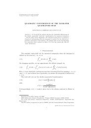
ON THE LAPLACE TRANSFORM OF THE PSI FUNCTION
M. LAWRENCE GLASSER AND DANTE MANNA
Abstract. Guided by numerical experimentation, we have been able to prove that
Z
8 π/2 x 2
π 0 x 2 + ln 2 dx = 1 − γ + ln(2π)
[2cos(x)]
and to establish a connection with the Laplace transform of ψ(t + 1).
(1)
1. Introduction
Interest in this project began with curiosity about the Laplace transform of the Digamma function,
L(a) :=
∫ ∞
0
e −as ψ(s + 1)ds ,
which is conspicuously absent from the extensive literature and tabulations of Euler’s Gamma function.
As will be seen, this can be related to the odd logarithmic integral
(2)
M(a) :=
4 π
∫ π/2
0
x 2
x 2 + ln 2 (2e −a cos(x)) dx .
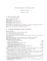
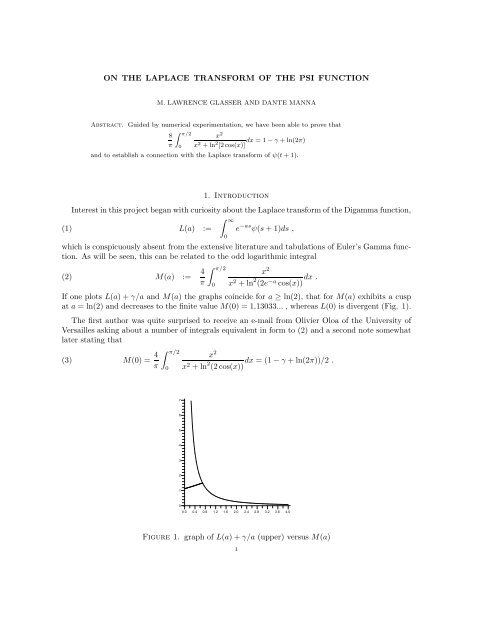
If one plots L(a) + γ/a and M(a) the graphs coincide for a ≥ ln(2), that for M(a) exhibits a cusp
at a = ln(2) and decreases to the finite value M(0) = 1.13033... , whereas L(0) is divergent (Fig. 1).
The first author was quite surprised to receive an e-mail from Olivier Oloa of the University of
Versailles asking about a number of integrals equivalent in form to (2) and a second note somewhat
later stating that
M(0) = 4 π
∫ π/2
0
x 2
x 2 + ln 2 dx = (1 − γ + ln(2π))/2 .
(2 cos(x))
(3)
4
7
6
5
3
2
1
0
0.0
0.4 0.8 1.2 1.6 2.0 2.4 2.8 3.2 3.6
4.0
Figure 1. graph of L(a) + γ/a (upper) versus M(a)
1

2 M. LAWRENCE GLASSER AND DANTE MANNA
Indeed this value had been guessed by making the reasonable assumption based on the connection
with the Gamma function that the only transcendental numbers involved were Euler’s constant,
ln(2) and ln(π). By examining the expression E(a, b, c, d) = a + bγ + c ln(2) + d ln(π) systematically
for small rational values of the coefficients precisely the above value was obtained. At the time our
note is written, this identity also appears in [8].
The aim of this note is to provide the details of the relation between L(a) and M(a) and to derive
the value of M(0). We present two proofs of the evaluation M(0), as well as a sum formula for the
integral. The general form of (1) for real parameter a appears to be
L(a) = M(a) − γ a − ln(ea − 1)
H(ln 2 − a) ,
1 − e−a where H denotes the unit step function. Oloa [7] has derived a conjecture for the general evaluation
of the related integral M(a) for all real a > 0 which has been confirmed by numerical experiments.
The derivation we present for the identity (3) in Section 2 begins by equating the integral in (2)
with the form
M(a) = πe −a ∫ 1
0
te −at
Γ(1 − t)
∑
k−l≠1
Γ(l − t)Γ(l − k − 1)
(1 − e a ) k dt .
l!Γ(l − k)
When a = 0, the hypergeometric sum reduces to a 3 F 2 , and we conclude the evaluation by appealing
to known evaluations of the ψ function.
In Section 3, we start by simplifying the integrand via a partial fractions decomposition and
change of variables. This results in a much simpler-looking integrand:
∫ π
y 2 dy
0 y 2 + 4 ln 2 (2 cos( y 2 )) = i ∫ π
(4) y dy
4 −π log(e iy + 1) .
The transformation e iy ↦→ z in the right hand integral would be the next logical step, because it
transforms the interval (−π, π) to a simple, closed contour in C that encircles the origin. However,
doing so from (4) would introduce complex logarithms in the integrand. To compensate for this,
we replace the integrand with an analytic integral and reverse order of integration. The result is to
reduce (3) to the evaluations
∫ 1
0
ln Γ(t) dt = ln( √ 2π) and (ln Γ) ′ (2) ≡ ψ(2) = 1 − γ .
Definite integrals on [0, 1] involving ln(Γ(x)) such as this have appeared in earlier research of Espinosa
and Moll; see [2], [4], [5] for details. We refer the reader to [9] for the analysis background concerning
our steps of simplification that involve, for example, passing a sum through an integral or analytic
continuation.
From (4) we can also make a series expansion of the integrand and integrate termwise, yielding
the formula
∫ (
)
π
y 2 dy
0 y 2 + 4 log 2 (2 cos( y 2 )) = π ∞∑ (−1) m m+1
∑ S 1 (m + 1, s)
(5)
1 +
.
2 m(m + 1)! s + 1
m=1
s=0
The S 1 (m, s) are signed Stirling numbers of the first kind, which appear when one writes a power
series expansion for 1/ log(1 + x) . We thus have, in view of (3), a new series evaluation.

ON THE LAPLACE TRANSFORM OF THE PSI FUNCTION 3
2. Derivation of the Logarithmic Integral
We begin by proving that the integrals L(a) + γ/a and M(a) agree for a > ln(2) . The former
diverges for all other real values of a , so that the latter is seen as its analytic continuation. To start,
formula (1.6.27) in [3] reads
Hence
(6)
B(y) =
= π 4
∫ π/2
0
cos(xy)cos s (x)dx = 2 −s−1 Γ(s + 1)
π
Γ(1 + 1 2 s + 1 2 y)Γ(1 + 1 2 s − 1 2 y) .
∫ π/2
0
2 −s Γ(s + 1)
[
Γ(1 + 1 2 s + 1 2 y)Γ(1 + 1 2 s − 1 2 y) ψ
xsin(xy)cos s (x)dx = −B ′ (y)
(
1 + s 2 + y ) (
− ψ 1 + s 2 2 − y )]
2
This generalizes Entry 33(i) in [1]. Therefore, evaluating at y = s , we obtain the integral representation
ψ(s + 1) = 2s+2
π
∫ π/2
0
xsin(sx)cos s (x)dx − γ .
Substituting this into the previous expression, we obtain the double integral
(7)
L(a) + γ a = 4 π
∫ ∞
Writing sin(sx) = − Im(e −isx ) , this becomes
Now the integral
L(a) + γ a = − 4 π Im ∫ ∞
∫ ∞
0
0
∫ π/2
e −(a−ln 2)s xsin(sx)cos s (x) dx ds.
0
∫ π/2
0
0
xe s(ln[2e−a cos(x)]−ix) dx ds.
e s(ln[2e−a cos(x)]−ix) ds for 0 < x < π/2
is equal to 1/(ix − ln[2e −a cos(x)]) when a > ln 2 and does not converge for any other values of a .
Thus, with this restriction in place, we may reverse the order of integration, yielding
L(a) + γ a = − 4 π Im ∫ π/2
0
x
ix − ln[2e −a cos(x)]
dx = M(a) .
Then, for 0 < a ≤ ln 2, we have M(a) as an alternative branch value of the function L(a) + γ/a.
Now we retrace the our steps slightly differently, starting from (7). For fixed s > 0 , the imaginary
part of integrand with respect to x is even; we write
M(a) = 2 π Im ∫ ∞
0
∫ π/2
−π/2
xe s ln[2e−a cos(x)] e isx dx ds .
Then using the functional equation e isx e sln[2e−a cos x] = e sln[e−a (1+e 2ix )] and the change of variables
x ↦→ x/2 yields
M(a) = 1
2π Im ∫ ∞
0
∫ π
As before, we have that the s-integral evaluates to
∫ ∞
0
e sln[e−a (1+e ix )] =
−π
xe s ln[e−a (1+e ix )] dx ds .
−1
ln[e −a (1 + e ix )]
when a > ln 2 ,
.

4 M. LAWRENCE GLASSER AND DANTE MANNA
and diverges otherwise. Since the parameter a is already restricted to the region of the former
inequality, we have that
Employing the general identity
M(a) = − 1
2π Im ∫ π
1
lnf
in the case f = e −a (e ix + 1) , leads to the form
M(a) = − 1
2π ea Im
∫ 1
0
=
−π
xdx
ln[e −a (1 + e ix )] .
∫ 1
0
e −at ∫ π
−π
f t
f − 1 dt ,
xe −ix (1 + e ix ) t
1 − (e a dx dt.
− 1)e−ix Next we expand in powers of e ix and take the imaginary part to obtain
M(a) = − 1 ∫ 1 ∑
∞ ( ) ∫ t π
π ea e −at (e a − 1) k xsin(l − k − 1)x dx dt .
l
0
k,l=0
The x-integral is easily worked out and vanishes if l − k = 1. The binomial coefficient can be
expressed using Gamma functions, leading to
∫ 1
M(a) = e a te −at ′∑ Γ(l − t)Γ(l − k − 1)
(8)
(e a − 1) k dt ,
Γ(1 − t) l!Γ(l − k)
0
where the prime on the sum denotes that terms with l − k = 1 are excluded. The sum represents
a hypergeometric function of two variables, which strongly suggests that for general values of a no
further progress is possible.
However, for a = 0 only terms with k = 0 contribute. Hence,
∫ [
1
∞
]
t ∑ Γ(l − t)Γ(l − 1)
M(0) =
− Γ(−t)
Γ(1 − t) l!Γ(l)
0
l=2
Finally, the sum can be evaluated in terms of a generalized hypergeometric function leading to
M(0) = 1 2
∫ 1
0
t(1 − t) 3 F 2 (1, 1, 2 − t; 2, 3; 1) dt + 1 .
The hypergeometric function does not appear to be tabulated, but experimenting with MATHE-
MATICA leads to
3F 2 (1, 1, 2 − t; 2, 3; 1) = 2 [1 − γ − ψ(t + 1)] ,
1 − t
and since [6] ∫ 1
0 xψ(x + 1)dx = 1 − ln √ 2π we have proven that
∫ π/2
0
x 2
x 2 + ln 2 [2 cos(x)] dx = π [1 − γ + ln(2π)] .
8
Evaluations of the integral M(a) for nonzero values of a still appear to be possible. Oloa’s
conjectured representations for M(a) differs from (8) in that the only functions of a involved are
natural logarithms, exponentials and objects of the form
∫ 1
0
0
e at ln Γ(t) dt .
We refer the reader to [7] for details and consequences of his remarkable formulae.
dt .

ON THE LAPLACE TRANSFORM OF THE PSI FUNCTION 5
3. Other Evaluations of M(0)
This section gives the details of the calculations of the second derivation as described in the
introduction, beginning with a proof of (4).
Proposition 3.1.
∫ π
0
y 2 dy
y 2 + 4 ln 2 (2 cos( y 2 )) = i ∫ π
y dy
4 −π log(e iy + 1) ,
where the logarithm in the denominator of the right-hand integral takes the principal value.
Proof. We move from the integral on the left to the integral on the right using a change of variables.
To begin, we factor the ( denominator of the integrand on the left,
( y
[ ( ( y
][ ( ( y
]
y 2 + 4 ln 2 2 cos = 2 ln 2 cos + iy 2 ln 2 cos − iy
2))
2))
2))
and expand the integrand into partial fractions. Then we split into two integrals, one for each term
of the decomposition:
(9)
∫ π
0
y 2 ∫
dy
π
y 2 + 4 ln 2 (2 cos( y 2 )) = g(y) dy −
0
∫ π
0
g(−y) d(−y) ,
where
iy
g(y) :=
4 ln(2 cos( y .
2
)) + 2iy
Now we transform the second integral on the right hand side of (9) by y ↦→ −y and combine with
the first one to get
Then write
∫ π
0
y 2 ∫
dy
π
y 2 + 4 ln 2 (2 cos( y 2 )) =
−π
iy dy
4 ln(2 cos( y .
2
)) + 2iy
( ( [ y (
2 ln 2 cos = log e
2))
iy/2 + e −iy/2) ] 2
= 2 log ( e iy + 1 ) − iy
for y ∈ (−π, π), where the logarithm function in the middle and right formulas takes the principal
value. This leads directly to the desired conclusion.
□
Next, we provide an evaluation of the integral in terms of an infinite sum. This is done by
expanding the integrand in a power series and then integrating termwise. We first provide a proof
of this expansion.
Proposition 3.2. For all z ∈ C \ {0} ,
(10)
1
∞
log(1 + z) = ∑
m=0
z m−1
m!
m∑
s=0
S 1 (m, s)
s + 1
=
∞∑
m=0
b m
z m−1
m!
where the S 1 (m, s) are signed Stirling numbers of the first kind and the b m are Bernoulli numbers
of the second kind.
Proof. Begin by observing that
∫
z 1
log(1 + z) = (z + 1) t dt
m=0
0
for all complex z ≠ 0 . The integrand on the right can be expanded using the binomial theorem,
∞∑
(z + 1) t z m
(11)
Γ(t + 1)
=
m! Γ(t − m + 1) ,
,

6 M. LAWRENCE GLASSER AND DANTE MANNA
which converges uniformly in t ∈ [0, 1] for all complex z . The coefficients of this power series are
polynomials in t:
Γ(t + 1)
m
Γ(t − m + 1) ≡ ∑
S 1 (m, s)t s .
s=0
The integers S 1 (m, s) in the above formula are Stirling numbers of the first kind, which are implicitly
defined for 0 ≤ m ≤ s by the above relation. Therefore
z
∞
log(1 + z) = ∑ z m ∫ 1
Γ(t + 1)
∞
m! Γ(t − m + 1) dt = ∑ z m m∑ S 1 (m, s)
(12)
,
m! s + 1
m=0
0
and we finish by dividing everywhere by z . The second identity is even more immediate, in view of
the definition of Bernoulli numbers of the second kind:
b n :=
∫ 1
0
m=0
s=0
Γ(t + 1)
dt , for n ∈ {0, 1, 2, ...} .
Γ(t − n + 1)
Combine this with the middle expression in (12) and then divide by z.
Now we evaluate the original integral as an infinite series.
Proposition 3.3.
(13)
∫ π
0
0
y 2 dy
y 2 + 4 log 2 (2 cos( y 2 )) = π 2
(
1 +
∞∑ (−1) m
m(m + 1)!
(
m=1
= π 2
1 +
m+1
∑
s=0
∞∑
m=1
)
S 1 (m + 1, s)
s + 1
)
(−1) m b m+1
m(m + 1)!
Proof. Using the power series (10) with z = e iy for y ∈ [−π, π] and applying this to the integral in
(4) gives
∫ π
y 2 dy
y 2 + 4 log 2 (2 cos( y 2 )) = i ∞∑ 1
m∑
∫
S 1 (m, s) π
(14)
ye i(m−1)y dy .
4 m! s + 1
m=0
We are justified in bringing the integral within the infinite sum, since the argument e iy is within the
radius of convergence of the power series. The integrals
evaluate to (−1) m+1 × 2πi
m
way to see this is to verify that
I m :=
∫ π
−π
s=0
ye imy dy , m ∈ Z
for all integers m ≠ 0, and 0 in the exceptional case. The most direct
d
dy
−π
( 1 − imy
m 2 e imy )
= ye imy for m ≠ 0
and evaluate at the endpoints. To complete the proof, substitute this value into (14).
Finally we prove the numerically-confirmed result (3).
□
□
Proposition 3.4.
∫ π
0
y 2 dy
y 2 + 4 ln 2 (2 cos( y 2 )) = π (1 − γ + ln(2π)) .
4

ON THE LAPLACE TRANSFORM OF THE PSI FUNCTION 7
Proof. Start with (4) and the integral
i
4
∫ π
−π
y dy
log(e iy + 1) ,
where we take the principle value of the complex logarithm. We write the integrand as
∫
iy
1
(
log(e iy + 1) = − d (e iy + 1) t
(15)
dt .
ds
For fixed t, s ∈ N such that t > s, we integrate
F(s, t) := − 1 4
∫ π
−π
0
(e iy + 1) t
e iys
e iys )s=1
dy = − 1 4i
∫
C
(z + 1) t
z s+1
where C is the simple, closed counterclockwise path around the unit circle in the complex plane.
The integrand is clearly analytic in a neighbornood of this path, as its only singularity lies at z = 0 .
By the residue theorem, the value of this contour integral is 2πi times the integrand’s residue at
z = 0. The Laurent expansion of the integrand is
∞∑
(z + 1) t
z s+1 =
m=0
Γ(t + 1)
Γ(m + 1)Γ(t − m + 1) zm−s−1 ,
using a similar binomial expansion to the one in (11). In this expansion we use the gamma function,
the extension of the factorial which is defined for all complex arguments with positive real part by
the integral
(16)
Γ(n) :=
∫ ∞
From the series above we draw the evaluation
0
x n−1 e −x dx , Γ(n + 1) = n! for n ∈ N .
F(s, t) = − π 2
Γ(t + 1)
Γ(s + 1)Γ(t − s + 1) .
In light of (16) we see the right hand side as an analytic continuation of the integral for all complex
parameters s and t (excluding negative integer values). Thus it is allowable to differentiate F with
respect to the parameter s . This gives us
where
∂F
∂s = −π 2
( )
(ψ(t − s + 1) − ψ(s + 1))Γ(t + 1)
,
Γ(s + 1)Γ(t − s + 1)
ψ(z) := Γ′ (z)
Γ(z) = d log(Γ(z)) for z ∈ C .
dz
Among well-known identities ([2], p. 212) for this classical function are
⎛ ⎞
n∑
ψ(2) = 1 − γ , where γ := lim ⎝
1
n→∞ j − ln(n) ⎠ ,
so that we have
∂F
∂s (1, t) = −π 2
( )
(ψ(t) − (1 − γ))Γ(t + 1)
Γ(t)
Finally, we integrate both sides on [0, 1]:
∫ 1
0
∂F
∂s (1, t) dt = −π 2
∫ 1
0
j=0
tψ(t) dt + π 2
dz
= − πt (ψ(t) − (1 − γ)) .
2
∫ 1
0
(1 − γ)t dt .

8 M. LAWRENCE GLASSER AND DANTE MANNA
Using integration by parts to compute the right hand side, we get
π
2
∫ 1
0
log Γ(t) dt + π (1 − γ) .
4
The remaining integral is famously ([6] and on the cover of [2]!) known to be ln( √ 2π) .
This gives us
∫ 1
(
d
− − 1 ∫ π
(e iy + 1) t )
0 ds 4 −π e iys dy dt = π (1 − γ + ln(2π)) .
s=1
4
To finish, we notice that the integral in the variable y that represents F(s, t) is uniformly convergent
in neighborhoods of s = 1 and t ∈ [0, 1] . Thus the integral can be viewed as a holomorphic function
of the parameters in that region. Therefore, we can change the order of the differentiation by s and
the integration over y, and switch the order of integration in the variables t and y. With (15) the
result is
∫
i π
4 −π
and in view of (4) this gives the desired identity.
y dy
log(e iy + 1) = π (1 − γ + ln(2π)) ,
4
Finally, we have a sum evaluation as a corollary.
□
Corollary 3.5.
∞∑ (−1) m b m+1
=
m(m + 1)!
m=1
∞∑
m=1
(−1) m m+1
∑ S 1 (m + 1, s)
m(m + 1)! s + 1
s=0
Proof. This follows from combining identities (3) and (5).
= 1 2
( )
ln(2π) − 1 − γ .
□
With the aid of symbolic and numerical calculators, we have proven a new evaluation for a
logarithmic integral and connected this to the Laplace transform of Psi function and a Stirling
series. We conclude by mentioning the other role technology has played in the formation of this
paper. Our collaboration itself is digital, done internationally (and overseas) via email; as of the
date of submission the authors have not yet met face to face.
Acknowedgements. The first author thanks the University of Valladolid for hospitality while this
work was carried out. The second author acknowledges J. Borwein for helpful comments and the
support of the AARMS Director’s Postdoctoral Fellowship.
References
[1] B. Berndt. Ramanujan’s Notebooks, Part I. Springer-Verlag, New York, 1985.
[2] G. Boros and V. Moll. Irresistible Integrals. Cambridge University Press, New York, 1st edition, 2004.
[3] A. Erdélyi. Tables of Integral Transforms, volume 1. McGraw-Hill, New York, 1st edition, 1954.
[4] O. Espinosa and V. Moll. On Some Definite Integrals Involving the Hurwitz Zeta Function. Part 1. Ramanujan
Journal, 6:159–188, 2002.
[5] O. Espinosa and V. Moll. On Some Definite Integrals Involving the Hurwitz Zeta Function. Part 2. Ramanujan
Journal, 6:449–468, 2002.
[6] G. M. Fichtengolz. Course in Differential and Integral Calculus, volume 2. (Moscow 1948).
[7] O. Oloa. Some Euler-Type Integrals and a New Rational Series for Euler’s Constant, volume Proceedings of the
Special Session on Experimental Mathematics in Action of Contemporary Mathematics. American Mathematical
Society, 2007.
[8] Eric W. Weisstein. ”Definite Integral,” Mathworld – a Wolfram Web Resource.
http://mathworld.wolfram.com/DefiniteIntegral.html, Last updated: Jan. 25, 2007.
[9] E.T. Whittaker and G.N. Watson. Modern Analysis. Cambridge University Press, 1962.

ON THE LAPLACE TRANSFORM OF THE PSI FUNCTION 9
Department of Physics, Clarkson University, Potsdam, NY U. S. A. 13699-5820
E-mail address: laryg@clarkson.edu
Department of Mathematics and Statistics, Dalhousie University, Halifax, NS Canada B3H 3J5
E-mail address: dmanna@mathstat.dal.ca