Consequences of One Bit Quantization on Signal to ... - CASPER
Consequences of One Bit Quantization on Signal to ... - CASPER
Consequences of One Bit Quantization on Signal to ... - CASPER

You also want an ePaper? Increase the reach of your titles
YUMPU automatically turns print PDFs into web optimized ePapers that Google loves.
<strong>CASPER</strong> Memo 012<br />
<str<strong>on</strong>g>C<strong>on</strong>sequences</str<strong>on</strong>g> <str<strong>on</strong>g>of</str<strong>on</strong>g> <str<strong>on</strong>g>One</str<strong>on</strong>g> <str<strong>on</strong>g>Bit</str<strong>on</strong>g> <str<strong>on</strong>g>Quantizati<strong>on</strong></str<strong>on</strong>g> <strong>on</strong> <strong>Signal</strong> <strong>to</strong> Noise Ratio<br />
Daniel Chapman<br />
January 2007<br />
1 Background<br />
1.1 <strong>Signal</strong> <strong>to</strong> Noise Ratio (SNR)<br />
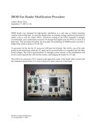
Imagine a set <str<strong>on</strong>g>of</str<strong>on</strong>g> time domain data that is composed <str<strong>on</strong>g>of</str<strong>on</strong>g> two elements:<br />
• a pure sine wave with RMS amplitude A and frequency f<br />
• and gaussian noise with a standard deviati<strong>on</strong> (or RMS amplitude) <str<strong>on</strong>g>of</str<strong>on</strong>g> B<br />
If we take the Fourier Transform <str<strong>on</strong>g>of</str<strong>on</strong>g> this data, we expect the resulting spectrum <strong>to</strong> be made up noise and<br />
<strong>on</strong>e spike located at frequency f. Example:<br />
(a) time domain (pre-fft)<br />
(b) frequency domain (post-fft)<br />
Figure 1: A sine wave with rms amplitude A=0.5 <strong>on</strong> <strong>to</strong>p <str<strong>on</strong>g>of</str<strong>on</strong>g> gaussian noise with standard deviati<strong>on</strong> B=1.0<br />
In the frequency domain data, the height <str<strong>on</strong>g>of</str<strong>on</strong>g> the spike divided by the height <str<strong>on</strong>g>of</str<strong>on</strong>g> the noise is known as the<br />
signal <strong>to</strong> noise ratio. Naturally, as you increase the strength <str<strong>on</strong>g>of</str<strong>on</strong>g> the sine wave relative <strong>to</strong> the gaussian noise<br />
(i.e. increase A/B) in your time domain data, you will increase the signal <strong>to</strong> noise ratio in your frequency<br />
domain data.<br />
1
1.2 <str<strong>on</strong>g>Quantizati<strong>on</strong></str<strong>on</strong>g><br />
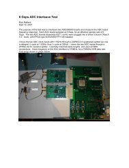
Now let’s imagine what happens when you quantize the input signal in<strong>to</strong> a <strong>on</strong>e bit number, where the bit<br />
simply represents whether the signal is positive or negative. Although the data loses a t<strong>on</strong> <str<strong>on</strong>g>of</str<strong>on</strong>g> precisi<strong>on</strong>, you<br />
can still make out the original sine wave (see Figure 2).<br />
(a) time domain data, unquantized<br />
(b) same data, quantized<br />
Figure 2: A sine wave with rms amplitude A=1.4 <strong>on</strong> <strong>to</strong>p <str<strong>on</strong>g>of</str<strong>on</strong>g> gaussian noise with standard deviati<strong>on</strong> B=1.0<br />
So, how does quantizati<strong>on</strong> affect the signal <strong>to</strong> noise ratio When A/B is small, the signal <strong>to</strong> noise ratio<br />
will be low regardless <str<strong>on</strong>g>of</str<strong>on</strong>g> whether or not the input is quantized. As we slowly increase A/B, the sine wave<br />
will become more obvious in both data sets, just as you can identify the sine wave in both plots in figure 2<br />
(although it is a little less clear in the quantized data).<br />
As A/B becomes large, however, the quantized data s<strong>to</strong>ps improving. Imagine the difference between<br />
input data with A/B=100 and A/B=1000. In both cases, the quantized data will look like a square wave.<br />
In c<strong>on</strong>trast, unquantized data with A/B=1000 will produce a much larger signal <strong>to</strong> noise ratio than data<br />
with A/B=100, because the magnitude <str<strong>on</strong>g>of</str<strong>on</strong>g> sine wave is preserved. Thus, where the SNR from unquantized<br />
data c<strong>on</strong>tinues <strong>to</strong> rise as we increase A/B, the SNR from quantized data quickly levels <str<strong>on</strong>g>of</str<strong>on</strong>g>f.<br />
2 Results<br />
How do we quantify this With a program that loops over A/B, calculating the SNR at each value.<br />
The C code at the end <str<strong>on</strong>g>of</str<strong>on</strong>g> this document produces the data for the plots <strong>on</strong> the next page. The X-axis<br />
correspends <strong>to</strong> A/B (signal RMS amplitude / noise RMS amplitude), and the Y-axis corresp<strong>on</strong>ds <strong>to</strong> the<br />
square root <str<strong>on</strong>g>of</str<strong>on</strong>g> the power <str<strong>on</strong>g>of</str<strong>on</strong>g> the signal divided by the power <str<strong>on</strong>g>of</str<strong>on</strong>g> the noise.<br />
The first plot display how the SNR increases for both quantized and unquantized data. The sec<strong>on</strong>d plot<br />
divides the two curves, giving you an idea <str<strong>on</strong>g>of</str<strong>on</strong>g> where the two curves diverge.<br />
2
Figure 3: SNR vs. A/B for both quantized and unquantized data<br />
Figure 4: quantized/unquantized curves representing SNR vs. A/B<br />
3
#include <br />
#include <br />
#include <br />
#define ARRAY_SIZE 1000<br />
/* From the GNU Scientific Library, src/randist/gauss.c<br />
Polar (Box-Mueller) method; See Knuth v2, 3rd ed, p122 */<br />
double rand_uniform(){<br />
/* return uniform (-1 <strong>to</strong> 1) */<br />
double value;<br />
value = 2.0 * (((double) rand()) / ((double) RAND_MAX)) - 1.0;<br />
return value;<br />
}<br />
double gsl_ran_gaussian (c<strong>on</strong>st double sigma)<br />
{<br />
double x, y, r2;<br />
do{<br />
/* choose x,y in uniform square (-1,-1) <strong>to</strong> (+1,+1) */<br />
x = -1 + 2 * rand_uniform();<br />
y = -1 + 2 * rand_uniform();<br />
/* see if it is in the unit circle */<br />
r2 = x * x + y * y;<br />
}while (r2 > 1.0 || r2 == 0);<br />
/* Box-Muller transform */<br />
return sigma * y * sqrt (-2.0 * log (r2) / r2);<br />
}<br />
double quantize(double value){<br />
if(value < 0)<br />
return -1.0;<br />
else<br />
return 1.0;<br />
}<br />
int main(){<br />
int i,j,k, num_k_loops;<br />
double SNR[ARRAY_SIZE];<br />
double spectrum_i;<br />
double gauss;<br />
double A_signal;<br />
double sum_signal, sum_noise;<br />
FILE *fp_output;<br />
srand(time(NULL));<br />
num_k_loops = 100;<br />
for(j=0; j
just <strong>on</strong>e frequency comp<strong>on</strong>ent since we know what frequency we expect<br />
the spike <strong>to</strong> be in. To obtain the RMS power <str<strong>on</strong>g>of</str<strong>on</strong>g> the noise, we simply<br />
use power_time_domain = power_frequency_domain. */<br />
}<br />
for(k=0; k