a review of basic probability theory from another course I teach

Chapter 6 

A Summary of Probability and 

Statistics 

Collected here are a few basic definitions and ideas. Fore more details consult a textbook 

on probability or mathematical statistics, for instance [Sin91], [Par60], and [Bru65]. 

We begin with a discussion of discrete probabilites, which involves counting sets. Then 

we introduce the notion of a numerical valued random variable and random physical 

phenomena. The main goal of this chapter is to develope the tools we need to characterize 

the uncertainties in both geophysical data sets and in the description of Earth 

models—at least when we have our Bayesian hats on. So the chapter culminates with a 

discussion of various descriptive statistics numerical data (means, variances, etc). Most 

of the problems that we face in geophysics involves spatially or temporally varying 

random phenomena, also known as stochastic processes; e.g., velocity as a function of 

space. For everything we will do in this course, however, it suffices to consider only finite 

dimensional vector-valued random variables, such as we would measure by sampling a 

random function at discrete times or spatial locations. 

6.1 Sets 

Probability is fundamentally about measuring sets. The sets can be finite, as in the 

possible outcomes of a toss of a coin, or infinite, as in the possible values of a measured 

P-wave impedance. The space of all possible outcomes of a given experiment is called 

the sample space. We will usually denote the sample space by Ω. If the problem is 

simple enough that we can enumerate all possible outcomes, then assigning probabilities 

is easy. 

0

72 A Summary of Probability and Statistics 

Ω 

A 

B 

C 

A U (B - C) 

C - B 

B C 

Ω - (A U B U C) 

U 

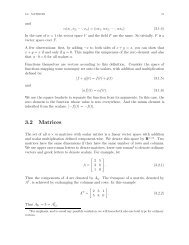
Figure 6.1: Examples of the intersection, union, and complement of sets. 

Example 1 

Toss a fair die twice. By “fair” we mean that each of the 6 possible outcomes is equally 

likely. The sample space for this experiment consists of {1, 2, 3, 4, 5, 6}. There are six 

possible equally likely outcomes of tossing the die. There is only one way to get any 

given number 1 − 6, therefore if A is the event that we toss a 4, then the probability 

associated with A, which we will call P (A) is 

P (A) = N(A) 

N(Ω) = 1 6 

(6.1) 

where we use N(A) to denote the number of possible ways of achieving event A and 

N(Ω) is the size of the sample space. 

6.1.1 More on Sets 

The union of two sets A and B consists of all those elements which are either in A or 

B; this is denoted by A ∪ B or A + B The intersection of two sets A and B consists of 

all those elements which are in both A and B; this is denoted by A ∩ B or simply AB. 

The complement of a set A relative to another set B consists of those elements which 

are in A but not in B; this is denoted by A − B. Often, the set B is this relationship 

is the entire sample space, in which case we speak simply of the complement of A and 

denote this by A c . These ideas are illustrated in Figure 6.1 

0

6.1 Sets 73 

The set with no elements in it is called the empty set and is denoted ∅. Its probability 

is always 0 

P (∅) = 0. (6.2) 

Since, by definition, the sample space contains all possible outcomes, its probability 

must always be 1 

P (Ω) = 1. (6.3) 

The other thing we need to be able to do is combine probabilities: a 

P (A ∪ B) = P (A) + P (B) − P (AB). (6.4) 

P (AB) is the probability of the event A intersect B, which means the event A and B. 

In particular, if the two events are exclusive, i.e., if AB = 0 then 

P (A ∪ B) = P (A) + P (B). (6.5) 

This result extends to an arbitrary number of exclusive events A i 

n∑ 

P (A 1 ∪ A 2 ∪ · · · ∪ A n ) = P (A i ). (6.6) 

i=1 

This property is called additivity. 

P (AB) = P (A)P (B). 

Events A and B are said to be independent if 

Example 2 

Toss the fair die twice. The sample space for this experiment consists of 

{{1, 1}, {1, 2}, . . . {6, 5}, {6, 6}}. (6.7) 

Let A be the event that the first number is a 1. Let B be the event that the second 

number is a 2. The the probability of both A and B occurring is the probability of the 

intersection of these two sets. So 

P (AB) = N(AB) 

N(Ω) 

= 1 36 

(6.8) 

Example 3 

A certain roulette wheel has 4 numbers on it: 1, 2, 3, and 4. The even numbers are 

white and the odd numbers are black. The sample space associated with spinning the 

wheel twice is 

{{1, 1}, {1, 2}, {1, 3}, {1, 4}} 

a That P (A ∪ B) = P (A) + P (B) for exclusive events is a fundamental axiom of probability. 

0


{{2, 1}, {2, 2}, {2, 3}, {2, 4}} 

{{3, 1}, {3, 2}, {3, 3}, {3, 4}} 

{{4, 1}, {4, 2}, {4, 3}, {4, 4}} 

Now, in terms of black and white, the different outcomes are 

{{black, black}, {black, white}, {black, black}, {black, white}} 

{{white, black}, {white, white}, {white, black}, {white, white}} 

{{black, black}, {black, white}, {black, black}, {black, white}} 

{{white, black}, {white, white}, {white, black}, {white, white}} 

Let A be the event that the first number is white, and B the event that the second 

number is white. Then N(A) = 8 and N(B) = 8. So P (A) = 8/16 and P (B) = 8/16. 

The event that both numbers are white is the intersection of A and B and P (AB) = 

4/16. 

Suppose we want to know the probability of the second number being white given that 

the first number is white. We denote this conditional probability by P (B|A). The only 

way for this conditional event to be true if both B and A are true. Therefore, P (B|A) 

is going to have to be equal to N(AB) divided by something. That something cannot 

be N(Ω) since only half of these have a white number in the first slot, so we must divide 

by N(A) since these are the only events for which the event B given A could possibly 

be true. Therefore we have 

P (B|A) = N(AB) 

N(A) 

= P (AB) 

P (A) 

(6.9) 

assuming P (A) is not zero, of course. The latter equality holds because we can divide 

the top and the bottom of N(AB) by N(Ω). 

N(A) 

As we saw above, for independent events P (AB) = P (A)P (B). Therefore it follows 

that for independent events P (B|A) = P (B). 

6.2 Random Variables 

If we use a variable to denote the outcome of a random trial, then we call this a random 

variable. For example, let d denote the outcome of a flip of a fair coin. Then d is 

a random variable with two possible values, heads and tails. A given outcome of a 

random trial is called a realization. Thus if we flip the coin 100 times, the result is 100 

realizations of the random variable d. Later in this book we will find it necessary to 

invent a new notation so as to distinguish a realization of a random process from the 

random process itself, the later being usually unknown. 

0

6.2 Random Variables 75 

6.2.1 A Definition of Random 

It turns out to be difficult to give a precise mathematical definition of randomness, so 

we won’t try. (A brief perusal of randomness in Volume 2 of Knuth’s great The Art of 

Computer Programming is edifying and frustrating in equal measures.) In any case it is 

undoubtedly more satisfying to think in terms of observations of physical experiments. 

Here is Parzen’s (1960) definition, which is as good as any: 

A random (or chance) phenomenon is an empirical phenomenon characterized 

by the property that its observation under a given set of circumstances 

does not always lead to the same observed outcomes (so that there is no 

deterministic regularity) but rather to different outcomes in such a way that 

there is statistical regularity. By this is meant that numbers exist between 

0 and 1 that represent the relative frequency with which the different possible 

outcomes may be observed in a series of observations of independent 

occurrences of the phenomenon. ... A random event is one whose relative 

frequency of occurrence, in a very long sequence of observations of randomly 

selected situations in which the event may occur, approaches a stable limit 

value as the number of observations is increased to infinity; the limit value 

of the relative frequency is called the probability of the random event 

It is precisely this lack of deterministic reproducibility that allows us to reduce random 

noise by averaging over many repetitions of the experiment. 

6.2.2 Generating random numbers on a computer 

Typically computers generate “pseudo-random” numbers according to deterministic 

recursion relations called Congruential Random Number Generators, of the form 

X(n + 1) = (aX(n) + c) mod m (6.10) 

where a and b are constants and m is called the modulus. (E.g., 24 = 12 (mod 12).) 

The value at the step n is determined by the value and step n − 1. 

The modulus defines the maximum period of the sequence; but the multiplier a and the 

shift b must be properly chosen in order that the sequence generate all possible integers 

between 0 and m − 1. For badly chosen values of these constants there will be hidden 

periodicities which show up when plotting groups of k of these numbers as points in 

k-dimensional space. 

To implement Equation 6.10 We need four magic numbers: 

• m, the modulus m > 0 

0


• a, the multiplier 0 ≤ a < m 

• c, the increment 0 ≤ c < m 

• X(0), the starting value (seed) 0 ≤ X(0) < m. 

Here’s an example. Take X(0) = a = c = 7 and take m = 10. Then the sequence of 

numbers generated by our recursion is: 

7, 6, 9, 0, 7, 6, 9, 0, ... 

Woops. The sequence begins repeating on the fourth iteration. This is called a periodicity. 

Fortunately, for better choices of the magic numbers, we can generate sequences 

that do not repeat until n is quite large. Perhaps as large as 2 64 or larger. But in all 

cases, such linear congruential “random number” generators are periodic. 

A large portion of Volume II of Knuth’s treatise on computer programming [Knu81] 

is devoted to computer tests of randomness and to theoretical defintions. We will not 

discuss here how good choices of the magic numbers are made, except to quote Theorem 

A, from section 3.2.1.2, volume 2 of [Knu81]. 

Theorem 8 The linear congruential sequence defined by m, a, c, and X(0) has period 

length m if and only if 

• c is relatively prime to m [i.e., if the greatest common divisor of c and m is 1] 

• b = a − 1 is a multiple of p, for every prime p dividing m 

• b is a multiple of 4, if m is a multiple of 4. 

In any case, the key point is that when you use a typical random number generator, 

you are tapping into a finite sequence of numbers. The place where you jump into 

the queue is called the seed. The sequence is purely deterministic (being generated by 

recursion), and we must rely on some other analysis to see whether or not the numbers 

really do look “random.” 

This led to a famous quote by one of the fathers of modern computing: 

Anyone who considers arithmetical methods of producing random digits is, of course, 

in a state of sin. – John von Neumann (1951) 

Any deterministic number generator, such as the recursion above, which is designed 

to mimic a random process (i.e., to produce a sequence of numbers with no apparent 

pattern) is called a pseudo-random number generator (PRNG). Virtually all of the 

0

6.2 Random Variables 77 

so-called random number generators used today are in fact pseudo-random number 

generators. This may seem like an minor point until you consider that many important 

numerical algorithms (so-called Monte Carlo methods) rely fundamentally on being 

able to make prodigious use of random numbers. Unsuspected periodicities in pseudorandom 

number generators have led to several of important physics papers being called 

into question. 

Can we do better than PRNG Yes and no. Yes we can, but not practically at the 

scale required by modern computing. To see a pretty good random process, watch the 

lottery drawing on TV some time. State lotteries usually make use of the classic “well 

stirred urn”. How about aiming an arrow at a distant target. Surely the spread of the 

arrows is random. In fact, one of the words we use for random phenomena (stochastic) 

comes from a Greek word which means to aim. Or tune your radio to an unallocated 

channel and listen to the static. Amplify this static, feed it through an A/D board into 

your computer and voila: random numbers. Suspend a small particle (a grain of pollen 

for instance) in a dish of water and watch the particle under a microscope. (This is 

called Brownian motion, after Robert Brown, the 19th century Scottish botanist who 

discovered it.) Turn on a Geiger counter (after Hans Geiger, the 20th century German 

physicist) near some source of radioactivity and measure the time between clicks. Put 

a small marker in a turbulent fluid flow, then measure the position of the marker. 

The fluctuations in sea height obtained from satellite altimetry. There are countless 

similarly unpredictable phenomena, but the question is: could we turn any of these into 

useful RNG It’s been tried (see Knuth, 1973). But the appetite of modern physical 

means of computing random numbers may not be able to keep up with the voracious 

needs of Monte Carlo computer codes. Further, we would have to store all the numbers 

in a big table so that we could have them to reuse, else we couldn’t debug our codes 

(they wouldn’t be repeatable). 

Under Linux, true random numbers are available by reading /dev/random. This generator 

gathers environmenal noise (from hardware devices, such as mouse movements, 

keystrokes, etc.) and keeps track of how much disorder (entropy) is available. When 

the entropy pool is empty, further reads to /dev/random will be blocked. (For more 

information see the man page for random.) This means that the number of strong random 

numbers is limited; it may be inadequate for numerical simulations, such as Monte 

Carlo calculuations, that require vast quantities of such numbers. For a more extensive 

discussion of “true radom numbers” see the web page www.random.org, from which you 

can download true random numers or surf to other sites that provide them. 

0


Here is a simple Scilab function for generating normally distributed pseudo-random 

numbers, by transforming uniformly distributed numbers. 

function [z] = gaussiansamples(n,m,s) 

// returns n pseudorandom samples from a normal distribution 

// with mean m and standard deviation s. This is based on the 

// Box-Muller transformation algorithm which is well-known to 

// be a poor choice. 

uniform1 = rand(n,1); 

uniform2 = rand(n,1); 

Pi = atan(1) * 4; 

gauss1 = cos(Pi * uniform1) .* sqrt(-2 * log(uniform2)); 

// gauss2 = sin(2 *Pi * uniform1) .* sqrt(-2 * log(uniform2)); 

z = (s .* gauss1) + m; 

// you can return the 2n samples generated by using gauss2 if you want 

6.3 Bayes’ Theorem 

Above we showed with a simple example that the conditional probability P (B|A) was 

given by 

Let’s write this as 

P (B|A) = N(AB) 

N(A) 

= P (AB) 

P (A) . (6.11) 

P (AB) = P (B|A)P (A). (6.12) 

Now, the intersection of A and B is clearly the same as the intersection of B and A. 

So P (AB) = P (BA). Therefore 

P (AB) = P (B|A)P (A) = P (BA) = P (A|B)P (B). (6.13) 

So we have the following relations between the two different conditional probabilities 

P (A|B) and P (B|A) 

P (A|B)P (B) 

P (B|A) = . (6.14) 

P (A) 

and 

P (A|B) = 

P (B|A)P (A) 

. (6.15) 

P (B) 

0

6.4 Probability Functions and Densities 79 

These are known as Bayes’ theorem. 

Suppose we have n mutually exclusive and exhaustive events C i . By mutually exclusive 

we meant that the intersection of any two of the C i is the empty set (the set with no 

elements) 

C i C j = ∅. (6.16) 

By exhaustive we meant that the union of all the C i fills up the entire sample space 

(i.e., the certain event) 

C 1 ∪ C 2 ∪ · · · ∪ C n = Ω. (6.17) 

It is not difficult to see that for any event B, we have 

P (B) = P (BC 1 ) + P (BC 2 ) + · · · P (BC n ). (6.18) 

You can think of this as being akin to writing a vector as the sum of its projections 

onto orthogonal (independent) directions (sets). Since the C i are independent and 

exhaustive, every element in B must be in one of the intersections BC i ; and no element 

can appear in more than one. Therefore B = BC 1 ∪ · · · BC n , and the result follows 

from the additivity of probabilities. Finally, since we know that for any C i P (BC i ) = 

P (B|C i )P (C i ) it follows that 

P (B) = P (B|C 1 )P (C 1 ) + P (B|C 2 )P (C 2 ) + · · · P (B|C n )P (C n ). (6.19) 

This gives us the following generalization of Bayes’ Theorem 

P (C i |B) = P (BC i) 

P (B) 

= 

P (B|C i )P (C i ) 

∑ nj=1 

P (B|C j )P (C j ) . (6.20) 

Thomas Bayes (1702-1761) is best known for his theory of probability 

outlined in his Essays towards solving a problem in the doctrine 

of chances published in the Philosophical transactions of the Royal 

Society (1763). He wrote a number of other mathematical essays but 

none were published during his lifetime. Bayes was a nonconcormist 

minister who preached at the Presbyterian Chapel in Turbridge Wells 

(south of London) for over 30 years. He was elected a fellow of the 

Royal Society in 1742. 

6.4 Probability Functions and Densities 

So far in this chapter we have dealt only with discrete probabilities. The sample space 

Ω has consisted of individual events to which we can assign probabilities. We can 

assign probabilities to collections of events by using the rules for the union, intersection 

and complement of events. So the probability is a kind of measure on sets. 1) It’s 

0


Figure 6.2: The title of Bayes’ article, published posthumously in the Philosophical 

Transactions of the Royal Society, Volume 53, pages 370–418, 1763 

Figure 6.3: Bayes’ statement of the problem. 

0


always positive, 2) it’s zero on the null set (the impossible event), 3) it’s one on the 

whole sample space (the certain event), 4) and it satisfies the additivity property for 

an arbitrary collection of mutually independent events A i : 

P (A 1 ∪ A 2 ∪ · · · ∪ A n ) = P (A 1 ) + P (A 2 ) + · · · P (A n ). (6.21) 

These defining properties of a probability function are already well known to us in 

other contexts. For example, consider a function M which measures the length of a 

subinterval of the unit interval I = [0, 1]. If 0 ≤ x 1 ≤ x 2 ≤ 1, then A = [x 1 , x 2 ] is a 

subinterval of I. Then M(A) = x 2 − x 1 is always positive unless the interval is empty, 

x 1 = x 2 , in which case it’s zero. If A = I, then M(A) = 1. And if two intervals are 

disjoint, the measure (length) of the union of the two intervals is the sum of the length 

of the individual intervals. So it looks like a probability function is just a special kind 

of measure, a measure normalized to one. 

Now let’s get fancy and write the length of an interval as the integral of some function 

over the interval. 

∫ 

∫ x2 

M(A) = µ(x) dx ≡ µ(x) dx. (6.22) 

A 

x 1 

In this simple example using cartesian coordinates, the density function µ is equal to a 

constant one. But it suggests that more generally we can define a probability density 

such that the probability of a given set is the integral of the probability density over 

that set 

∫ 

P (A) = ρ(x) dx (6.23) 

or, more generally, 

∫ 

P (A) = 

A 

A 

ρ(x 1 , x 2 , . . . , x n ) dx 1 dx 2 · · · dx n . (6.24) 

Of course there is no reason to restrict ourselves to cartesian coordinates. The set 

itself is independent of the coordinates used and we can transform from one coordinate 

system to another via the usual rules for a change of variables in definite integrals. 

Yet another representation of the probability law of a numerical valued random phenomenon 

is in terms of the distribution function F (x). F (x) is defined as the probability 

that the observed value of the random variable will be less than x: 

F (x) = P (X < x) = 

∫ x 

−∞ 

ρ(x ′ ) dx ′ . (6.25) 

Clearly, F must go to zero as x goes to −∞ and it must go to one as x goes to +∞. 

Further, F ′ (x) = ρ(x). 

Example 

∫ ∞ 

−∞ 

e −x2 dx = √ π. (6.26) 

0


This integral is done on page 110. Let Ω be the real line −∞ ≤ x ≤ ∞. Then 

ρ(x) = √ 1 

π 

e −x2 is a probability density on Ω. The probability of the event x ≥ 0, is 

then 

P (x ≥ 0) = √ 1 ∫ ∞ 

e −x2 dx = 1 π 2 . (6.27) 

The probability of an arbitrary interval I ′ is 

0 

P (x ∈ I ′ ) = 1 √ π 

∫I ′ e −x2 dx (6.28) 

Clearly, this probability is positive; it is normalized to one 

P (−∞ ≤ x ≤ ∞) = 1 √ π 

∫ ∞ 

the probability of an empty interval is zero. 

−∞ 

e −x2 dx = 1; (6.29) 

6.4.1 Expectation of a Function With Respect to a Probability 

Law 

Henceforth, we shall be interested primarily in numerical valued random phenomena; 

phenomena whose outcomes are real numbers. A probability law for such a phenomena 

P , can be thought of as determining a (in general non-uniform) distribution of a unit 

mass along the real line. This extends immediately to vector fields of numerical valued 

random phenomena, or even functions. Let ρ(x) be the probability density associated 

with P , then we define the expectation of a function f(x) with respect to P as 

E[f(x)] = 

∫ ∞ 

−∞ 

f(x)ρ(x) dx. (6.30) 

Obviously this expectation exists if and only if the improper integral converges. The 

mean of the probability P is the expectation of x 

E[x] = 

∫ ∞ 

−∞ 

xρ(x) dx. (6.31) 

For any real number ξ, we define the n-th moment of P about ξ as E[(x − ξ) n ]. The 

most common moments are the central moments, which correspond to E[(x− ¯x) n ]. The 

second central moment is called the variance of the probability law. 

Keep in mind the connection between the ordinary variable x and the random variable 

itself; let us call the latter X. Then the probability law P and the probability density 

p are related by 

P (X < x) = 

∫ x 

−∞ 

ρ(x ′ ) dx ′ . (6.32) 

We will summarize the basic results on expectations and variances later in this chapter. 

0


6.4.2 Multi-variate probabilities 

We can readily generalize a one-dimensional distribution such 

P (x ∈ I 1 ) = 1 √ π 

∫I 1 

e −x2 dx, (6.33) 

where I 1 is a subset of R 1 , the real line, to two dimensions: 

P ((x, y) ∈ I 2 ) = 1 π 

∫ ∫ 

I 2 

e −(x2 +y 2) dx dy (6.34) 

where I 2 is a subset of the real plane R 2 . So ρ(x, y) = 1 +y 2) is an example of a joint 

π e−(x2 

probability density on two variables. We can extend this definition to any number of 

variables. In general, we denote by ρ(x 1 , x 2 , ...x N ) a joint density for the N-dimensional 

random variable. Sometimes we will write this as ρ(x). By definition, the probability 

that the N−vector x lies in some subset A of R N is given by: 

∫ 

P [x ∈ A] = ρ(x) dx (6.35) 

where dx refers to some N−dimensional volume element. 

A 

independence 

We saw above that conditional probabilities were related to joint probabilities by 

P (AB) = P (B|A)P (A) = P (A|B)P (B) 

from which result Bayes theorem follows. The same result holds for random variables. 

If a random variable X is independent of event Y , so that the probability of Y does not 

depend on the probability of X. That is, P (x|y) = P (x) and P (y|x) = P (y). Hence 

for independent events, P (x, y) = P (x)P y). 

Once we have two random variables X and Y , with a joint probability P (x, y), we can 

think of their moments. The joint n − m moment of X and Y about 0 is just 

∫ ∫ 

E[x n y m ] = 

x n y m ρ(x, y)dxdy. (6.36) 

The 1-1 moment about zero is called the correlation of the two random variables: 

∫ ∫ 

Γ XY = E[xy] = xyρ(x, y)dxdy. (6.37) 

On the other hand, the 1-1 moment about the means is called the covariance: 

C XY = E[(x − E(x))(y − E(y)) = Γ XY − E[x]E[y]. (6.38) 

0


The covariance and the correlation measure how similar the two random variables are. 

This similarity is distilled into a dimensionless number called the correlation coefficient: 

where σ X is the variance of X and σ Y is the variance of Y . 

r = C XY 

σ X σ Y 

(6.39) 

Using Schwarz’s inequality, namely that 

∫ ∫ 

2 ∫ ∫ 

∣ f(x, y)g(x, y)dxdy 

∣ ≤ 

∫ ∫ 

|f(x, y)| 2 dxdy 

|g(x, y)| 2 dxdy (6.40) 

and taking 

and 

it follows that 

√ 

f = (x − E(x)) (ρ(x, y)) 

√ 

g = (y − E(x)) (ρ(x, y)) 

|C XY | ≤ σ x σ y . (6.41) 

This proves that 0 ≤ r ≤ 1. A correlation coefficient of 1 means that the fluctuations in 

X and Y are essentially identical. This is perfect correlation. A correlation coefficient 

of -1 means that the fluctuations in X and Y are essentially identical but with the 

opposite sign. This is perfect anticorrelation. A correlation coefficient of 0 means X 

and Y are uncorrelated. 

Two independent random variables are always uncorrelated. But dependent random 

variables can be uncorrelated too. 

Here is an example from [Goo00]. Let Θ be uniformly distributed on [−π/2, π/2]. Let 

X = cos Θ and Y = sin Θ. Since knowledge of Y completely determines X, these two 

random variables are clearly dependent. But 

. 

C XY = 1 π 

∫ π/2 

−π/2 

cos θ sin θdθ = 0 

marginal probabilities 

From an n−dimensional joint distribution, we often wish to know the probability that 

some subset of the variables take on certain values. These are called marginal probabilities. 

For example, from ρ(x, y), we might wish to know the probability P (x ∈ I 1 ). 

To find this all we have to do is integrate out the contribution from y. In other words 

P (x ∈ I 1 ) = 1 π 

∫I 1 

∫ ∞ 

0 

−∞ 

e −(x2 +y 2) dx dy. (6.42)


covariances 

The multidimensional generalization of the variance is the covariance. Let ρ(x) = 

ρ(x 1 , x 2 , ...x n ) be a joint probability density. The the i−j components of the covariance 

matrix are defined to be: 

∫ 

C ij (m) = (x i − m i )(x j − m j )ρ(x) dx (6.43) 

where m is the mean of the distribution 

∫ 

m = 

xρ(x) dx. (6.44) 

Equivalently we could say that 

C = E[(x − m)(x − m) T ]. (6.45) 

From this definition it is obvious that C is a symmetric matrix. The diagonal elements 

of the covariance matrix are just the ordinary variances (squares of the standard 

deviations) of the components: 

C ii (m) = (σ i ) 2 . (6.46) 

The off-diagonal elements describe the dependence of pairs of components. 

As a concrete example, the n-dimensional normalized gaussian distribution with mean 

m and covariance C is given by 

[ 

1 

ρ(x) = 

(2π det C) exp − 1 ] 

N/2 2 (x − m)T C −1 (x − m) . (6.47) 

This result and many other analytic calculations involving multi-dimensional Gaussian 

distributions can be found in [MGB74] and [Goo00]. 

An aside, diagonalizing the covariance 

Since the covariance matrix is symmetric, we can always diagonalize it with an orthogonal 

transformation involving real eigenvalues. It we transform to principal coordinates 

(i.e., rotate the coordinates using the diagonalizing orthogonal transformation) then the 

covariance matrix becomes diagonal. So in these coordinates correlations vanish since 

they are governed by the off-diagonal elements of the covariance matrix. But suppose 

one or more of the eigenvalues is zero. This means that the standard deviation of that 

parameter is zero; i.e., our knowledge of this parameter is certain. Another way to say 

this is that one or more of the parameters is deterministically related to the others. This 

is not a problem since we can always eliminate such parameters from the probabilistic 

description of the problems. Finally, after diagonalizing C we can scale the parameters 

by their respective standard deviations. In this new rotated, scaled coordinate system 

the covariance matrix is just the identity. In this sense, we can assume in a theoretical 

analysis that the covariance is the identity since in priciple we can arrange so that it is. 

0


6.5 Random Sequences 

Often we are faced with a number of measurements {x i } that we want to use to estimate 

the quantity being measured x. A seismometer recording ambient noise, for example, 

is sampling the velocity or displacement as a function of time associated with some 

piece of the earth. We don’t necessarily know the probability law associated with the 

underlying random process, we only know its sampled values. Fortunately, measures 

such as the mean and standard deviation computed from the sampled values converge 

to the true mean and standard deviation of the random process. 

The sample average or sample mean is defined to be 

¯x ≡ 1 N 

N∑ 

x i 

i=1 

sample moments: Let x 1 , x 2 , ...x N be a random random sample from the probability 

density ρ. Then the rth sample moment about 0, is given by 

1 

N 

N∑ 

x r i . 

i=1 

If r = 1 this is the sample mean, ¯x. Further, the rth sample moment about ¯x, is given 

by 

M r ≡ 1 N∑ 

(x i − ¯x) r . 

N 

i=1 

How is the sample mean ¯x related to the mean of the underlying random variable 

(what we will shortly call the expectation, E[X]) This is the content of the law of 

large numbers; here is one form due to Khintchine (see [Bru65] or [Par60]): 

Theorem 9 Khintchine’s Theorem: If ¯x is the sample mean of a random sample of 

size n from the population induced by a random variable x with mean µ, and if ɛ > 0 

then: 

P [‖¯x − µ‖ ≥ ɛ] → 0 as n → ∞. 

In the technical language of probability the sample mean ¯x is said to converge in probability 

to the population mean µ. The sample mean is said to be an “estimator” of true 

mean. 

A related result is 

Theorem 10 Chebyshev’s inequality: If a random variable X has finite mean ¯x and 

0

6.5 Random Sequences 87 

-5 -4 -3 -2 -1 0 1 2 3 4 5 

Figure 6.4: A normal distribution of zero mean and unit variance. Almost all the area 

under this curve is contained within 3 standard deviations of the mean. 

variance σ 2 , then [Par60]: 

for any ɛ > 0. 

P [‖X − ¯x‖ ≤ ɛ] ≥ 1 − σ2 

ɛ 2 

This says that in order to make the probability of X being within ɛ of the mean greater 

σ 

than some value p, we must choose ɛ at least as large as √ 1−p 

. Another way to say this 

would be: let p be the probability that x lies within a distance ɛ of the mean ¯x. Then 

σ 

Chebyshev’s inequality says that we must choose ɛ to be at least as large as 

√ 1−p 

. 

For example, if p = .95, then ɛ ≥ 4.47σ, while for p = .99, then ɛ ≥ 10σ. For the normal 

probability, this inequality can be sharpened considerably: the 99% confidence interval 

is ɛ = 2.58σ. But you can see this in the plot of the normal probability in Figure 6.4. 

This is the standard normal probability (zero mean, unit variance). Clearly nearly all 

the probability is within 3 standard deviations. 

6.5.1 The Central Limit Theorem 

The other basic theorem of probability which we need for interpreting real data is this: 

the sum of a large number of independent, identically distributed random variables 

(defined on page 21), all with finite means and variances, is approximately normally 

distributed. This is called the central limit theorem, and has been known, more or 

less, since the time of De Moivre in the early 18-th century. The term “central limit 

theorem” was coined by George Polya in the 1920s. There are many forms of this result, 

for proofs you should consult more advanced texts such as [Sin91] and [Bru65]. 

0


100 Trials 1000 Trials 10000 Trials 

0.1 

0.08 

0.06 

0.04 

0.02 

0.08 

0.06 

0.04 

0.02 

0.08 

0.06 

0.04 

0.02 

12345678910 11 

13 14 15 16 17 18 19 20 21 22 23 24 25 26 27 28 29 30 31 32 33 34 35 36 37 38 39 40 41 42 43 44 45 46 47 48 49 50 51 52 53 54 55 56 57 58 59 60 61 62 63 64 65 66 67 68 69 70 71 72 73 74 75 76 77 78 79 80 81 82 83 84 85 86 87 88 89 90 91 92 93 94 95 96 97 98 100 99 

0 50 100 

12345678910 11 

13 14 15 16 17 18 19 20 21 22 23 24 25 26 27 28 29 30 31 32 33 34 35 36 37 38 39 40 41 42 43 44 45 46 47 48 49 50 51 52 53 54 55 56 57 58 59 60 61 62 63 64 65 66 67 68 69 70 71 72 73 74 75 76 77 78 79 80 81 82 83 84 85 86 87 88 89 90 91 92 93 94 95 96 97 98 100 99 

0 

12345678910 11 

13 14 15 16 17 18 19 20 21 22 23 24 25 26 27 28 29 30 31 32 33 34 35 36 37 38 39 40 41 42 43 44 45 46 47 48 49 50 51 52 53 54 55 56 57 58 59 60 61 62 63 64 65 66 67 68 69 70 71 72 73 74 75 76 77 78 79 80 81 82 83 84 85 86 87 88 89 90 91 92 93 94 95 96 97 98 100 99 

50 100 0 50 100 

Figure 6.5: Ouput from the coin-flipping program. The histograms show the outcomes 

of a calculation simulating the repeated flipping of a fair coin. The histograms have 

been normalized by the number of trials, so what we are actually plotting is the relative 

probability of of flipping k heads out of 100. The central limit theorem guarantees that 

this curve has a Gaussian shape, even though the underlying probability of the random 

variable is not Gaussian. 

Theorem 11 Central Limit Theorem: If ¯x is the sample mean of a sample of size n 

from a population with mean µ and standard deviation σ, then for any real numbers a 

and b with a < b 

[ 

P µ + √ aσ < ¯x < µ + bσ ] 

√ → 1 ∫ b 

√ e −z2 /2 dz. 

n n 2π 

This just says that the sample mean is approximately normally distributed. 

Since the central limit theorem says nothing about the particular distribution involved, 

it must apply to even something as apparently non-Gaussian as flipping a coin. Suppose 

we flip a fair coin 100 times and record the number of heads which appear. Now, repeat 

the experiment a large number of times, keeping track of how many times there were 0 

heads, 1, 2, and so on up to 100 heads. Obviously if the coin is fair, we expect 50 heads 

to be the peak of the resulting histogram. But what the central limit theorem says is 

that the curve will be a Gaussian centered on 50. 

This is illustrated in Figure 6.5 via a little code that flips coins for us. For comparison, 

the exact probability of flipping precisely 50 heads is 

a 

( ) 

100! 1 100 

≈ .076. (6.48) 

50!50! 2 

What is the relevance of the Central Limit Theorem to real data Here are three 

conflicting views quoted in [Bra90]. From Scarborough (1966): “The truth is that, for 

the kinds of errors considered in this book (errors of measurement and observation), 

the Normal Law is proved by experience. Several substitutes for this law have been 

proposed, but none fits the facts as well as it does.” 

From Press et al. (1986): “This infatuation [of statisticians with Gaussian statistics] 

tended to focus interest away from the fact that, for real data, the normal distribution 

0

6.6 Expectations and Variances 89 

is often rather poorly realized, if it is realized at all.” 

And perhaps the best summary of all, Gabriel Lippmann speaking to Henri Poincaré: 

“Everybody believes the [normal law] of errors: the experimenters because they believe 

that it can be proved by mathematics, and the mathematicians because they believe it 

has been established by observation.” 

6.6 Expectations and Variances 

Notation: we use E[x] to denote the expectation of a random variable with respect to 

its probability law f(x). Sometimes it is useful to write this as E f [x] if we are dealing 

with several probability laws at the same time. 

If the probability is discrete then 

If the probability is continuous then 

E[x] = ∑ xf(x). 

E[x] = 

∫ ∞ 

−∞ 

xf(x) dx. 

Mixed probabilities (partly discrete, partly continuous) can be handled in a similar way 

using Stieltjes integrals [Bar76]. 

We can also compute the expectation of functions of random variables: 

E[φ(x)] = 

∫ ∞ 

−∞ 

φ(x)f(x) dx. 

It will be left as an exercise to show that the expectation of a constant a is a (E[a] = a) 

and the expectation of a constant a times a random variable x is a times the expectation 

of x (E[ax] = aE[x]). 

Recall that the variance of x is defined to be 

where µ = E[x]. 

V (x) = E[(x − E(x)) 2 ] = E[(x − µ) 2 ] 

Here is an important result for expectations: E[(x − µ) 2 ] = E[x 2 ] − µ 2 . The proof is 

easy. 

E[(x − µ) 2 ] = E[x 2 − 2xµ + µ 2 ] (6.49) 

= E[x 2 ] − 2µE[x] + µ 2 (6.50) 

= E[x 2 ] − 2µ 2 + µ 2 (6.51) 

= E[x 2 ] − µ 2 (6.52) 

0


An important result that we need is the variance of a sample mean. For this we use 

the following lemma, the proof of which will be left as an exercise: 

Lemma 1 If a is a real number and x a random variable, then V (ax) = a 2 V (x). 

From this it follows immediately that 

V (¯x) = 1 n 2 

n ∑ 

i=1 

V (x i ). 

In particular, if the random variables are identically distributed, with mean µ then 

V (¯x) = σ 2 /n. 

6.7 Bias 

In statistics, the bias of an estimator of some parameter is defined to be the expectation 

of the difference between the parameter and the estimator: 

B[ˆθ] ≡ E[ˆθ − θ] (6.53) 

where ˆθ is the estimator of θ. In a sense, we want the bias to be small so that we have 

a faithful estimate of the quantity of interest. 

An estimator ˆθ is unbiased if E[ˆθ] = θ 

For instance, it follows from the law of large numbers that the sample mean is an 

unbiased estimator of the population mean. In symbols, 

However, the sample variance 

s 2 ≡ 1 N 

E[¯x] = µ. (6.54) 

N∑ 

(x i − ¯x) 2 (6.55) 

i=1 

turns out not to be unbiased (except asymptotically) since E[s 2 ] = n−1 

n 

σ2 . To get an 

unbiased estimator of the variance we use E[ n 

n−1 s2 ]. To see this note that 

s 2 = 1 n∑ 

i − ¯x) 

N 

i=1(x 2 = 1 ( ) 

∑ 

1 

n∑ 

x 2 i 

N 

− 2x i¯x + ¯x 2 = x 2 i − ¯x 2 . 

N 

i=1 

Hence the expected value of s 2 is 

i=1 

E[s 2 ] = 1 N 

n∑ 

E[x 2 i ] − E[¯x 2 ]. 

i=1 

0

6.7 Bias 91 

Using a previous result, for each of the identically distributed x i we have 

E[x 2 i ] = V (x) + E[x]2 = σ 2 + µ 2 . 

And 

So 

E[¯x 2 ] = V (¯x) + E[¯x] 2 = 1 n σ2 + µ 2 . 

E[s 2 ] = σ 2 + µ 2 − 1 n σ2 − µ 2 = n − 1 

n σ2 . 

Finally, there is the notion of the consistency of an estimator. An estimator ˆθ of θ is 

consistent if for every ɛ > 0 

P [|ˆθ − θ| < ɛ] → 1 as n → ∞. 

Consistency just means that if the sample size is large enough, the estimator will be 

close to the thing being estimated. 

Later on, when we talk about inverse problems we will see that bias represents a potentially 

significant component of the uncertainty in the results of the calculations. 

Since the bias depends on something we do not know, the true value of the unknown 

parameter, it will be necessary to use a priori information in order to estimate it. 

Mean-squared error, bias and variance 

The mean-squared error (MSE) for an estimator m of m T is defined to be 

MSE(m) ≡ E[(m − m T ) 2 ] = E[m 2 − 2mm T + m 2 T ] = ¯m 2 − 2 ¯mm T + m 2 T . (6.56) 

By doing a similar analysis of the variance and bias we have: 

and 

Bias(m) ≡ E[m − m T ] = ¯m − m T (6.57) 

Var(m) ≡ E[(m − ¯m) 2 ] = E[m 2 − 2m ¯m + ¯m 2 ] = ¯m 2 − ¯m 2 . (6.58) 

So you can see that we have: MSE = Var + Bias 2 . As you can see, for a given meansquared 

error, there is a trade-off between variance and bias. The following example 

illustrates this trade-off. 

Example: Estimating the derivative of a smooth function 

We start with a simple example to illustrate the effects of noise and prior information in 

the performance of an estimator. Later we will introduce tools from statistical decision 

theory to study the performance of estimators given different types of prior information. 

0


Suppose we have noisy observations of a smooth function, f, at the equidistant points 

a ≤ x 1 ≤ . . . ≤ x n ≤ b 

y i = f(x i ) + ɛ i , i = 1, ..., n, (6.59) 

where the errors, ɛ i , are assumed to be iid N(0, σ 2 ) b . We want to use these observations 

to estimate the derivative, f ′ . We define the estimator 

ˆf ′ (x mi ) = y i+1 − y i 

, (6.60) 

h 

where h is the distance between consecutive points, and x mi = (x i+1 +x i )/2. To measure 

the performance of the estimator (6.60) we use the mean square error (MSE), which is 

the sum of the variance and squared bias. The variance and bias of (6.60) are 

Var[ ˆf ′ (x mi )] = Var(y i+1) + Var(y i ) 

= 2σ2 

h 2 

h , 2 

Bias[ ˆf ′ (x mi )] ≡ E[ ˆf ′ (x mi ) − f ′ (x mi )] 

= f(x i+1) − f(x i ) 

− f ′ (x mi ) = f ′ (α i ) − f ′ (x mi ), 

h 

for some α i ∈ [x i , x i+1 ] (by the mean value theorem) . We need some information on f ′ 

to assess the size of the bias. Let us assume that the second derivative is bounded on 

[a, b] by M 

|f ′′ (x)| ≤ M, x ∈ [a, b]. 

It then follows that 

|Bias[ ˆf ′ (x mi )]| = |f ′ (α i ) − f ′ (x mi )| = |f ′′ (β i )(α i − β i )| ≤ Mh, 

for some β i between α i and x mi . As h → 0 the variance goes to infinity while the bias 

goes to zero. The MSE is bounded by 

2σ 2 

h 2 

≤ MSE[ ˆf ′ (x mi )] = Var[ ˆf ′ (x mi )] + Bias[ ˆf ′ (x mi )] 2 ≤ 2σ2 

h 2 + M 2 h 2 . (6.61) 

It is clear that choosing the smallest h possible does not lead to the best estimate; 

the noise has to be taken into account. The lowest upper bound is obtained with 

h = 2 1/4√ σ/M. The larger the variance of the noise, the wider the spacing between 

the points. 

We have used a bound on the second derivative to bound the MSE. It is a fact that some 

type of prior information, in addition to model (6.59), is required to bound derivative 

uncertainties. Take any smooth function, g, which vanishes at the points x 1 , ..., x n . 

Then, the function ˜f = f + g satisfies the same model as f, yet their derivatives could 

be very different. For example, choose an integer, m, and define 

[ ] 

2πm(x − x1 ) 

g(x) = sin 

. 

h 

b Independent, identically distributed random variables, normally distributed with mean 0 and variance 

σ 2 . 

0

6.8 Correlation of Sequences 93 

Then, f(x i ) + g(x i ) = f(x i ) and 

˜f ′ (x) = f ′ (x) + 2πm [ ] 

2πm(x − 

h cos x1 ) 

. 

h 

By choosing m large enough, we can make the difference, ˜f ′ (x mi ) − f ′ (x mi ), as large 

as we want; without prior information the derivative can not be estimated with finite 

uncertainty. 

6.8 Correlation of Sequences 

Many people think that “random” and uncorrelated are the same thing. Random 

sequences need not be uncorrelated. Correlation of sequences is measured by looking at 

the correlation of the sequence with itself, the autocorrelation. c If this is approximately 

a δ-function, then the sequence is uncorrelated. In a sense, this means that the sequence 

does not resemble itself for any lag other than zero. But suppose we took a deterministic 

function, such as sin(x), and added small (compared to 1) random perturbations to it. 

The result would have the large-scale structure of sin(x) but with a lot of random junk 

superimposed. The result is surely still random, even though it will not be uncorrelated. 

If the autocorrelation is not a δ-function, then the sequence is correlated. Figure 6.6 

shows two pseudo-random Gaussian sequences with approximately the same mean, 

standard deviation and 1D distributions: they look rather different. In the middle of 

this figure are shown the autocorrelations of these two sequences. Since the autocorrelation 

of the right-hand sequence drops off to approximately zero in 10 samples, we 

say the correlation length of this sequence is 10. In the special case that the autocorrelation 

of a sequence is an exponential function, the the correlation length is defined as 

the (reciprocal) exponent of the best-fitting exponential curve. In other words, if the 

autocorrelation can be fit with an exponential e −z/l , then the best-fitting value of l is 

the correlation length. If the autocorrelation is not an exponential, then the correlation 

length is more difficult to define. We could say that it is the number of lags of the 

autocorrelation within which the autocorrelation has most of its energy. It is often 

impossible to define meaningful correlation lengths from real data. 

A simple way to generate a correlated sequence is to take an uncorrelated one (this is 

what pseudo-random number generators produce) and apply some operator that correlates 

the samples. We could, for example, run a length-l smoothing filter over the 

uncorrelated samples. The result would be a series with a correlation length approximately 

equal to l. A fancier approach would be to build an analytic covariance matrix 

and impose it on an uncorrelated pseudo-random sample. 

c From the convolution theorem, it follows that the autocorrelation is just the inverse Fourier transform 

of the periodogram (absolute value squared of the Fourier transform). 

0


0.75 

0.5 

0.25 

0.75 

0.5 

0.25 

-0.25 

-0.5 

-0.75 

-1 

1 

200 400 600 800 1000 

-0.25 

-0.5 

-0.75 

-1 

1 

200 400 600 800 1000 

0.8 

0.8 

0.6 

0.6 

0.4 

0.4 

0.2 

0 

0 10 20 

0.2 

0 

0 10 20 

200 

200 

150 

150 

100 

100 

50 

50 

1 2 3 4 5 6 7 8 9 10 11 12 13 14 

1 2 3 4 5 6 7 8 9 10 11 12 13 14 

Standard Deviation = .30 

Mean = 0 

Standard Deviation = .30 

Mean = 0 

Figure 6.6: Two Gaussian sequences (top) with approximately the same mean, standard 

deviation and 1D distributions, but which look very different. In the middle of this 

figure are shown the autocorrelations of these two sequences. Question: suppose we 

took the samples in one of these time series and sorted them in order of size. Would 

this preserve the nice bell-shaped curve 

0

6.8 Correlation of Sequences 95 

For example, an exponential covariance matrix could be defined by C i,j = σ 2 e −‖i−j‖/l 

where σ 2 is the (in this example) constant variance and l is the correlation length. 

To impose this correlation on an uncorrelated, Gaussian sequence, we do a Cholesky 

decomposition of the covariance matrix and dot the lower triangular part into the 

uncorrelated sequence [Par94]. If A is a symmetric matrix, then we can always write 

A = LL T , 

where L is lower triangular [GvL83]. This is called the Cholesky decomposition of 

the matrix A. You can think of the Cholesky decomposition as being somewhat like 

the square root of the matrix. Now suppose we apply this to the covariance matrix 

C = LL T . Let x be a mean zero pseudo-random vector whose covariance is the identity. 

We will use L to transform x: z ≡ Lx. The covariance of z is given by 

Cov(z) = E[zz T ] = E[(Lx)(Lx) T ] = LE[xx T ]L T = LIL T = C 

which is what we wanted. 

Here is a simple Scilab code that builds an exponential covariance matrix C i,j = 

σ 2 e −‖i−j‖/l and then returns n pseudo-random samples drawn from a Gaussian process 

with this covariance (and mean zero). 

function [z] = correlatedgaussian(n,s,l) 

// returns n samples of an exponentially correlated gaussian process 

// with variance s^2 and correlation length l. 

// first build the covariance matrix. 

C = zeros(n,n); 

for i = 1:n 

for j = 1:n 

C(i,j) = s^2 * exp(-abs(i-j)/l); 

end 

end 

L = chol(C); 

x = rand(n,1,’normal’); 

z = L*x; 

We would call this, for example, by: 

z = correlatedgaussian(200,1,10); 

0


The vector z should now have a standard deviation of approximately 1 and a correlation 

length of 10. To see the autocorrelation of the vector you could do: 

plot(corr(z,200)) 

the autocorrelation function will be approximately exponential for short lags. For longer 

lags you will see oscillatory departures from exponential behavior—even though the 

samples are drawn from an analytic exponential covariance. This is due to the small 

number of realizations. From the exponential part of the autocorrelation you can estimate 

the correlation length by simply looking for the point at which the autocorrelation 

has decayed by 1/e. Or you can fit the log of the autocorrelation with a straight line. 

6.9 Random Fields 

If we were to make N measurements of, say, the density of a substance, we could plot 

these N data as a function of the sample number. This plot might look something 

like the top left curve in Figure 6.6. But these are N measurements of the same thing, 

unless we belive that the density of the sample is changing with time. So a histogram of 

the measurements would approximate the probability density function of the parameter 

and that would be the end of the story. 

On the other hand, curves such as those in Figure 6.6 might result from measuring a 

random, time-varying process. For instance, these might be measurements of a noisy 

seismometer, in which case the plot would be N samples of voltage versus time. But 

then these would not be N measurements of the same parameter, rather they would be a 

single measurement of a random function, sampled at N different times. The distinction 

we are making here is the distinction between a scalar-valued random process and a 

random function. Now when we measure a function we always measure it at a finite 

number of locations (in space or time). So our measurements of random function result 

in finite-dimensional random vectors. This is why the sampling of a time series of 

voltage, say, at N times, is really the realization of a N-dimensional random process. 

For such a process it is not sufficient to simply make a histogram of the samples. 

We need higher order characterizations of the probability law behind the time-series. 

This is the study of random fields or stochastic processes. Here we collect a few basic 

definitions and results on the large subject of random fields. Of course there is nothing 

special about time-series. We could also be speaking of random processes that vary in 

space. 

0

6.9 Random Fields 97 

6.9.1 Elements of Random Fields 

Here we set forth the basic notations having to do with random functions. This section 

is an adaptation of Pugachev [Pug65] and is included primarily for the sake of completeness. 

Feel free to skip on the first reading. We will consider random fields in (3-D) 

physical space, adaptation to other sorts of fields is straightforward. 

Ξ(r) will denote a random field. A realization of the random field will be denoted 

by ξ(r) . We may think of ξ as a physical parameter defined at every point of the 

space (like the velocity of seismic waves, the temperature, etc.). We will work inside a 

volume V . 

n-dimensional joint probability densities 

Let (r 1 , r 2 , . . . , r n ) be a set of n points inside V . An expression like 

f n (ξ 1 , ξ 2 , . . . , ξ n ; r 1 , r 2 , . . . , r n ) 

will denote the n-dimensional (joint) probability density for the values ξ(r 1 ), ξ(r 2 ), . . . , ξ(r n ) . 

The notation f n (ξ 1 , ξ 2 , . . . , ξ n ; r 1 , r 2 , . . . , r n ) may seem complicated, but it just indicates 

that for every different set of points (r 1 , r 2 , . . . , r n ) we have a possibly different 

probability density. 

The random field Ξ(r) is completely characterized if, for any set of n points inside 

V , the joint probability density f n (ξ 1 , ξ 2 , . . . , ξ n ; r 1 , r 2 , . . . , r n ) is defined, and this for 

any value of n. 

Marginal and conditional probability 

The definitions for marginal and conditional probabilities do not pose any special difficulty. 

As notations rapidly become intricate, let us only give the corresponding definitions 

for some particular cases. 

If f 3 (ξ 1 , ξ 2 , ξ 3 ; r 1 , r 2 , r 3 ) is the 3-D joint probability for the values of the random field 

at points r 1 , r 2 and r 3 respectively, the marginal probability for the two points r 1 

and r 2 is defined by 

∫ 

f 2 (ξ 1 , ξ 2 ; r 1 , r 2 ) = 

dL(ξ 3 ) f 3 (ξ 1 , ξ 2 , ξ 3 ; r 1 , r 2 , r 3 ) , (6.62) 

where dL(ξ 3 ) is the (1-D) volume element (it may be dξ 3 

or something different). 

Let us now turn now to the illustration of the definition of conditional probability. If 

f 3 (ξ 1 , ξ 2 , ξ 3 ; r 1 , r 2 , r 3 ) is the 3-D joint probability for the values of the random field at 

0


points r 1 , r 2 and r 3 respectively, the conditional probability for the two points r 1 

and r 2 , given that the random field takes the value ξ 3 at point r 3 , is defined by 

i.e., using equation 6.62, 

f 3 (ξ 1 , ξ 2 , ξ 3 ; r 1 , r 2 , r 3 ) 

f 3 (ξ 1 , ξ 2 ; r 1 , r 2 |ξ 3 ; r 3 ) = ∫ dL(ξ3 ) f 3 (ξ 1 , ξ 2 , ξ 3 ; r 1 , r 2 , r 3 ) , (6.63) 

f 3 (ξ 1 , ξ 2 ; r 1 , r 2 |ξ 3 ; r 3 ) = f 3(ξ 1 , ξ 2 , ξ 3 ; r 1 , r 2 , r 3 ) 

f 2 (ξ 1 , ξ 2 ; r 1 , r 2 ) 

. (6.64) 

Of particular interest will be the one- and the two-dimensional probability densities, 

denoted respectively f 1 (ξ; r) and f 2 (ξ 1 , ξ 2 ; r 1 , r 2 ) . 

Random fields defined by low order probability densities 

First example: Independently distributed variables. 

If 

f n (ξ 1 , ξ 2 , . . . , ξ n ; r 1 , r 2 , . . . , r n ) = 

g(ξ 1 , r 1 ) h(ξ 2 , r 2 ) . . . i(ξ n , r n ) , (6.65) 

we say that the random field has independently distributed variables. 

Second example: Markov random field. 

For a Markov process, 

f n (ξ 1 , ξ 2 , . . . , ξ n ; r 1 , r 2 , . . . , r n ) = 

f 2 (ξ n ; r n |ξ n−1 ; r n−1 ) f 2 (ξ n−1 ; r n−1 |ξ n−2 ; r n−2 ) (6.66) 

. . . f 2 (ξ 2 ; r 2 |ξ 1 ; r 1 ) f 1 (ξ 1 ; r 1 ) , 

where the vertical bar denotes conditional probability. This means that the value at a 

given point depends only on the value at the previous point. As 

f 2 (ξ i ; r i |ξ i−1 ; r i−1 ) = f 2(ξ i−1 , ξ i ; r i−1 , r i ) 

f 1 (ξ i−1 ; r i−1 ) 

, (6.67) 

we obtain 

f n (ξ 1 , ξ 2 , . . . , ξ n ; r 1 , r 2 , . . . , r n ) = (6.68) 

f 2 (ξ 1 , ξ 2 ; r 1 , r 2 ) . . . f 2 (ξ n−1 , ξ n ; r n−1 , r n ) 

f 1 (ξ 2 ; r 2 ) f 1 (ξ 3 ; r 3 ) . . . f 1 (ξ n−1 ; r n−1 ) 

This equation characterizes a Markov random field in all generality. It means that the 

random field is completely characterized by 1-D and 2-D probability densities (defined 

at adjacent points). 

0 

.

6.9 Random Fields 99 

Third example: Gaussian random field. 

For a Gaussian random field, if we know the 2-D distributions, we know all the means 

and all the covariances, so we also know the n-dimensional distribution. It can be shown 

that a Gaussian process with exponential covariance is Markovian. 

Uniform random fields 

A random field is uniform (i.e., stationary) in the strong sense if for any r 0 , 

Taking 

gives then 

f n (ξ 1 , ξ 2 , . . . , ξ n ; r 1 , r 2 , . . . , r n ) = 

f n (ξ 1 , ξ 2 , . . . , ξ n ; r 0 + r 1 , r 0 + r 2 , . . . , r 0 + r n ) . 

r 0 = −r 1 

f n (ξ 1 , ξ 2 , . . . , ξ n ; r 1 , r 2 , . . . , r n ) = 

f n (ξ 1 , ξ 2 , . . . , ξ n ; 0, r 2 − r 1 , . . . , r n − r 1 ) . 

A distribution is said to be uniform in the weak sense if this expression holds only for 

n = 1 and n = 2. 

As the random field is defined over the physical space, we prefer the term uniform to 

characterize what, in random fields defined over a time variable, is called stationary. 

This is entirely a question of nomenclature; we regard the terms as being interchangeable. 

Example: 

For the two-dimensional distribution, 

f 2 (ξ 1 , ξ 2 ; r 1 , r 2 ) = Ψ 2 (ξ 1 , ξ 2 ; ∆r) , 

with 

∆r = r 2 − r 1 . 

Example: 

For the three-dimensional distribution, 

f 3 (ξ 1 , ξ 2 , ξ 3 ; r 1 , r 2 , r 3 ) = Ψ 3 (ξ 1 , ξ 2 , ξ 3 ; ∆r 1 , ∆r 2 ) . 

with 

∆r 1 = r 2 − r 1 

0


and 

∆r 2 = r 3 − r 1 . 

Essentially a uniform random process is one whose properties do not change with space 

(or time if that is the independent variable). 

Time versus statistical autocorrelation 

Given a known function u(t) (or this could be discrete samples of a known function 

u(t i )), the time autocorrelation function of u is defined as: 

∫ 

1 T/2 

˜Γ u (τ) = lim u(t + τ)u(t)dt. 

T ←∞ T −T/2 

This measures the similarity of u(t+τ) and u(t) averaged over all time. Closely related 

is the statistical autocorrelation function. Let U(t) be a random process. Implicity 

the random process consistutes the set of all possible sample functions u(t) and their 

associated probability measure. 

Γ u (t 1 , t 2 ) ≡ E[u(t 1 )u(t 2 )] = 

∫ ∞ 

−∞ 

∫ ∞ 

−∞ 

u 2 u 1 ρ U (u 1 , u 2 ; t 1 , t 2 )du 1 du 2 . 

Γ u (t 1 , t 2 ) measures the statistical similarity of u(t 1 ) and u(t 2 ) over the ensemble of all 

possible realizations of U(t). 

For stationary processes, Γ u (t 1 , t 2 ) depends only on τ ≡ t 2 − t 1 . 

processes: 

˜Γ(τ) = Γ u (τ) 

And for ergodic 

A real-data example of measurements of a random field is shown in Figure6.7. These 

traces represent 38 realizations of a time series recorded in a random medium. In this 

case the randomness is spatial: each realization is made at a different location in the 

medium. But you could easily imagine the same situation arising with a temporal 

random process. For example, these could be measurements of wave propagation in a 

medium undergoing random fluctuations in time, such as the ocean or the atmosphere. 

The way to think about this situation is that there is an underlying random process 

U(t), the probability law of which we do not know. To completely characterize the 

probability law of a stochastic process we must know the joint probability distribution 

ρ U (u 1 , u 2 , . . . , u n ; t 1 , t 2 , . . . , t n ) 

for all n. Of course we only make measurements of U at a finite numer of samples, so in 

practice we must know the n − th order rho U . d Now, the first-order PDF (probability 

d It is sometimes convenient to label the joint distribution by the random process, and sometimes 

0

6.10 Probabilistic Information About Earth Models 101 

0 

realization 

10 20 30 

0.05 

time (ms) 

0.10 

0.15 

0.20 

Figure 6.7: 38 realizations of an ultrasonic wave propagation experiment in a spatially 

random medium. Each trace is one realization of an unknown random process U(t). 

density function) is ρ U (u; t). Knowing this we can compute E[u], E[u 2 ], etc. The 

second-order PDF involves two times, t 1 and t 2 , and is the joint PDF of U(t 1 ) and 

U(t 2 ): ρ 2 (u 1 , u 2 ; t 1 , t 2 ), where u 1 = u(t 1 ) and u 2 = u(t 2 ). With this we can compute 

quantities such as: 

∫ ∫ 

E[u 1 u 2 ] = u 1 u 2 ρ U (u 1 , u 2 ; t 1 , t 2 )du 1 du 2 . 

6.10 Probabilistic Information About Earth Models 

In geophysics there is a large amount of a priori information that could be used to 

influence inverse calculations. Here, a priori refers to the assumption that this information 

is known independently of the data. Plausible geologic models can be based on 

rock outcrops, models of sedimentological deposition, subsidence, etc. There are also 

often in situ and laboratory measurements of rock properties that have a direct bearing 

on macroscopic seismic observations, such as porosity, permeability, crack orientation, 

etc. There are other, less quantitative, forms of information as well, the knowledge of 

experts for instance. 

There is a simple conceptual model that can be used to visualize the application of this 

diverse a priori information. Suppose we have a black box into which we put all sorts 

of information about our problem. We can turn a crank or push a button and out pops 

by the order as we did in the previous chapter. So, 

ρ U (u 1 , u 2 , . . . , u n ; t 1 , t 2 , . . . , t n ) ≡ ρ n (u 1 , u 2 , . . . , u n ; t 1 , t 2 , . . . , t n ) 

0


seismic data 

gravity data 

geology 

logs 

5 

6 

1 

4 

3 

2 

Earth model 1 

Earth model 2 

Earth model 3 

Earth model 4 

Figure 6.8: A black box for generating pseudo-random Earth models that agree with 

our a priori information. 

a model that is consistent with whatever information that is put in, as illustrated in 

Figure 6.8. 

If this information consists of an expert’s belief that, say, a certain sand/shale sequence 

is 90% likely to appear in a given location, then we must ensure that 90% of the models 

generated by the black box have this particular sequence. One may repeat the process 

indefinitely, producing a collection of models that have one thing in common: they are 

all consistent with the information put into the black box. 

Let us assume, for example, that a particular layered Earth description consists of 

the normal-incidence P-wave reflection coefficient r at 1000 different depth locations 

in some well-studied sedimentary basin. Suppose, further, that we know from in situ 

measurements that r in this particular sedimentary basin almost never exceeds .1. What 

does it mean for a model to be consistent with this information We can push the button 

on the black box and generate models which satisfy this requirement. Figure 6.9 shows 

some examples. 

The three models shown satisfy the hard constraint that |r| ≤ .1 but they look completely 

different. In the case of the two Gaussian models, we know this is because they 

have different correlation length. The real question is, which is most consistent with 

our assumed prior information What do we know about the correlation length in the 

Earth And how do we measure this consistency If we make a histogram of the in situ 

observations of r and it shows a nice bell-shaped curve, are we justified in assuming 

a Gaussian prior distribution On the other hand, if we do not have histograms of r 

0


White uniform 

0.1 

100 

0.05 

80 

60 

200 400 600 800 1000 40 

-0.05 

20 

-0.1 

1 2 3 4 5 6 7 8 9 10 

White Gaussian, mean = 0, std = .03 

0.05 

-0.05 

-0.1 

250 

200 

150 

200 400 600 800 1000 

100 

50 

1 2 3 4 5 6 7 8 9 10 

0.05 

-0.05 

-0.1 

Correlated Gaussian, mean = 0, std = .03, correlation length = 15 

250 

200 

150 

200 400 600 800 1000100 

50 

1 2 3 4 5 6 7 8 9 10 

Figure 6.9: Three models of reflectivity as a function of depth which are consistent with 

the information that the absolute value of the reflection coefficient must be less than 

.1. On the right is shown the histogram of values for each model. The top two models 

are uncorrelated, while the bottom model has a correlation length of 15 samples. 

0


Wave speed (m/s) 

2900 

2400 

1900 

0 500 1000 1500 2000 

Depth (m) 

Figure 6.10: Estimates of P and S wave velocity are obtained from the travel times 

of waves propagating through the formation between the source and receiver on a tool 

lowered into the borehole. 

but only extreme values, so that all we really know is that |r| ≤ .1, are we justified in 

thinking of this information probabilistically 

If we accept for the moment that our information is best described probabilistically, then 

a plausible strategy for solving the inverse problem would be to generate a sequence of 

models according to the prior information and see which ones fit the data. Assuming, of 

course, that we know the probability function that governs the variations of the Earth’s 

properties. In the case of the reflectivity sequence, imagine that we have surface seismic 

data to be inverted. For each model generated by the black box, compute synthetic 

seismograms, compare them to the data and decide whether they fit the data well 

enough to be acceptable. If so, the models are saved; if not, they are rejected. Repeating 

this procedure many times results in a collection of models that are, by definition, a 

priori reasonable and fit the data. If the models in this collection all look alike, then 

the features the models show are well-constrained by the combination of data fit and a 

priori information. If, on the other hand, the models show a diversity of features, then 

these features cannot be well-resolved. 

Information Naturally Suited to a Probabilistic Treatment 

Now let’s briefly consider the problem of how we would characterize the statistical 

properties of geophysical data. As an example, Figure 6.10 shows a sonic log, e which 

characterizes the short vertical wavelength (1 m or less) material fluctuations at a given 

location in the earth. Perhaps we can extract the statistical features of these data and 

use them to refine inferences made with other data sets from the same area. 

In order to focus on the statistical aspects of the data it is useful to subtract the longwavelength 

trend, which is likely the result of more gradual, deterministic changes such 

as compaction. The trend and the resulting fluctuations are shown in Figures 6.11 and 

6.12. This trend is our estimate of the mean of the random process, one realization of 

which we see in the log. 

e That is, an in situ estimate of acoustic wave speed as a function of depth inferred from travel times 

between a source and receiver in a measuring tool lowered into a well. NB, that the “data” are only 

indirectly measured, being, in fact, the result of an inference. This is a common situation in which 

there is no fundamental distinction between the input and the output of an inverse calculation. 

0


Wave speed (m/s) 

2900 

2400 

1900 

0 500 1000 1500 2000 

Depth (m) 

Figure 6.11: Trend of Figure 6.10 obtained with a 150 sample running average. 

Fluctuations (m/s) 

600 

400 

200 

0 

-200 

0 500 1000 1500 2000 

Depth (m) 

Figure 6.12: Fluctuating part of the log obtained by subtracting the trend from the log 

itself. 

1.0 

0.9 

Autocorrelation 

0.8 

0.7 

0.6 

0.5 

0.4 

0.3 

0.2 

0.1 

0.0 

0.0 20.0 40.0 60.0 80.0 100.0 

Lag (m) 

1 

0.5 

0 

80 100 

60 

20 40 

40 60 20 

80 100 

Figure 6.13: Autocorrelation and approximate covariance matrix (windowed to the first 

100 lags) for the well log. The covariance was computed according to Equation 6.69 

0


We know that a general N-dimensional random vector is characterized the the N- 

dimensional joint distribution function. However, we saw in the section on random 

fields, that for some random processeses the joint distribution function is itself completely 

characterized by some lower order moments of the distribution. For instance, 

if the fluctuations in the well log are stationary and Gaussian, the joint distribution 

function for the Earth velociy fluctuations is characterized by the mean and covariance. 

But how can we compute the covariance of a random field when we only have one 

realization (in this case the log) The short answer is that we cannot. Somehow we 

have to be able to average over the samples of log. The technical details can be found 

in [Pug65]. But the basic idea is to compute the autocorrelation of the fluctuations of 

the well log about the running mean within a sliding window. Using a sliding window 

accounts for the fact that both mean and variance of the well log change with depth. 

Once the correlation as a function of lag (C(τ)) is computed for a given window, the 

model covariance matrix is approximated by 

C [i, j] = C(j − i) 

= 

1 

N + 1 

i+ N 2 ∑ 

k=i− N 2 

L(k) L(k + j − i). (6.69) 

N is the length of the sliding window centered at depth i dz, L(k) is the well-log sample 

at depth k dz, and dz is the depth discretization interval. 

For example, Figure 6.13 shows the first 100 lags (1 meter per lag) of the correlation 

function for the fluctuating part of Figure 6.12, as well as an approximate covariance 

matrix. A slice along the diagonal of the covariance matrix, from the peak “downhill” 

is precisely the autocorrelation. So we’ve taken the one-dimensional autocorrelation 

and used it to approximate the two-dimensional covariance. If, on the other hand, we 

had many logs which supposedly sampled the same structure, then we could directly 

compute a sample covariance as 

where 

C = 1 N∑ 

(v i − ¯v)(v i − ¯v) T 

N 

i=1 

¯v = 1 N∑ 

v i . 

N 

i=1 

6.11 Other Common Analytic Distributions 

Finally, we close this chapter by mentioning a few other commonly used analytic distributions. 

Nearly as important theoretically as the Gaussian, is the lognormal distri- 

0

6.11 Other Common Analytic Distributions 107 

Figure 6.14: The lognormal is a prototype for asymmetrical distributions. It arises 

naturally when considering the product of a number of iid random variables. This 

figure was generated from Equation 6.70 for s = 2. 

bution. A variable X is lognormally distributed if Y = ln(X) is normally distributed. 

The central limit theorem treats the problem of sums of random variables; but the 

product of exponentials is the exponential of the sum of the exponents. Therefore we 

should expect that the lognormal would be important when dealing the a product of 

iid f random variables. One of these distributions, sketched in Figure 6.14, is the prototype 

of asymmetrical distributions. It also will play an important role later, when we 

talk about so-called non-informative distributions. In fact, there is a whole family of 

lognormal distributions given by 

[ 

1 

ρ(x) = 

sx √ 2π exp − 1 ( 

log x ) ] 2 

(6.70) 

2s 2 x 0 

where x 0 plays the analog of the mean of the distribution and s governs the shape. For 

small values of s (less than 1), the lognormal distribution is approximately gaussian. 

While for large values of s (greater than about 2.5), the lognormal approches 1/x. 

Figure 6.14 was computed for an s value of 2. 

The Gaussian distribution is a member of a family of exponential distributions referred 

to as generalized Gaussian distributions. Four of these distributions are shown in Figure 

6.15 for p = 1, 2, 10, and ∞. The p = 1 distribution is called the Laplacian or 

double-exponential, and the p = ∞ distribution is uniform. 

( 

ρ p (x) = 

p1−1/p −1 

2σ p Γ(1/p) exp |x − x 0 | p ) 

(6.71) 

p (σ p ) p 

where Γ is the Gamma function [MF53] and σ p is a generalized measure of variance 

known in the general case as the dispersion of the distribution: 

(σ p ) p ≡ 

f Independent, Identically Distributed. 

∫ ∞ 

−∞ 

|x − x 0 | p ρ(x) dx (6.72) 

0


p=1 

p=2 

p=10 

p=infinity 

Figure 6.15: The generalized Gaussian family of distributions. 

where x 0 is the center of the distribution. See [Tar87] for more details. 

0

6.11 Other Common Analytic Distributions 109 

Exercises 

1. Show that for any two events A and B 

2. Show that for any event A, P (A c ) = 1 − P (A). 

P (AB c ) = P (A) − P (BA) (6.73) 

3. Show that 1/x is a measure, but not a probability density. 

4. Show that the truth of the following formula for any two sets A and B 

P (A ∪ B) = P (A) + P (B) − P (A ∪ B) (6.74) 

follows from the fact that for independent sets A ′ and B ′ 

P (A ′ ∪ B ′ ) = P (A ′ ) + P (B ′ ). (6.75) 

Hint. The union of any two sets A and B can be written as the sum of three 

independent sets of elements: the elements in A but not in B; the elements in B 

but not in A; and the elements in both A and B. 

5. Show that all the central moments of the normal distribution beyond the second 

are either zero or can be written in terms of the mean and variance. 

6. You have made n different measurements of the mass of an object. You want 

to find the mass that best “fits” the data. Show that the mass estimator which 

minimizes the sum of squared errors is given by the mean of the data, while the 

mass estimator which minimizes the sum of the absolute values of the errors is 

given by the median of the data. Feel free to assume that you have an odd number 

of data. 

7. Show that Equation 6.47 is normalized. 

8. Take the n data you recorded above and put them in numerical order: x 1 ≤ x 2 ≤ 

... ≤ x n . Compute the sensitivity of the two different estimators, average and 

median, to perturbations in x n . 

What does this say about how least squares and least absolute values treat “outliers” 

in the data 

9. Find the normalization constant that will make 

a probability density on the real line. x 0 is a constant. 

What are the mean and variance 

p(x) = e −(x2 −x 0 x+x 2 0 ) (6.76) 

0


Answer: The exponential integral is ubiquitous. You should remember the following 

trick. 

Therefore 

[∫ ∞ 

H 2 = 

H 2 = 

e −x2 

−∞ 

∫ ∞ ∫ 2π 

0 

0 

H = 

] [∫ ∞ 

dx e −y2 

−∞ 

∫ ∞ 

e −x2 

−∞ 

e −r2 r dr dθ = 1 2 

dx 

] ∫ ∞ ∫ ∞ 

dy = e x2 +y 2 

−∞ −∞ 

∫ ∞ ∫ 2π 

0 

0 

e −ρ dρ dθ = π 

dx dy. 

So H = √ π 

More complicated integrals, such as 

∫ ∞ 

e −(x2 −xx 0 +x 2 0 ) dx 

−∞ 

appearing in the homework are just variations on a theme. First complete the 

square. So 

e −(x2 −xx 0 +x 2 0 ) = e −(x−x 0/2) 2 −3/4x 2 0 . 

And therefore 

∫ ∞ 

−∞ 

So the final result is that 

is a normalized probability. 

Now compute the mean. 

e −(x2 −xx 0 +x 2 0 ) dx = e −3/4x2 0 

= e −3/4x2 0 

∫ ∞ 

−∞ 

∫ ∞ 

e −(x−x 0/2) 2 

−∞ 

e −z2 dz = √ πe −3/4x2 0 . 

ρ(x) = 1 √ π 

e 3/4x2 0 e 

−(x 2 −xx 0 +x 2 0 ) 

¯x = √ 1 ∫ ∞ 

e 3/4x2 0 xe −(x2 −xx 0 +x 2 0 ) dx. 

π −∞ 

But this is not as bad as it looks since once we complete the sqaure, most of the 

normalization disappears 

dx 

¯x = 1 √ π 

∫ ∞ 

xe −(x−x 0/2) 2 

−∞ 

dx. 

Changing variables, we get 

¯x = 1 √ π 

∫ ∞ 

−∞ 

0 

(x + x 0 /2)e −x2 dx

a review of basic probability theory from another course I teach

Create successful ePaper yourself

Delete template?

Save as template?