Temperature and Pressure Measurements in a Turbine Engine
Temperature and Pressure Measurements in a Turbine Engine
Temperature and Pressure Measurements in a Turbine Engine

Create successful ePaper yourself
Turn your PDF publications into a flip-book with our unique Google optimized e-Paper software.
AE3051 Experimental Fluid Dynamics<br />
TEMPERATURE AND PRESSURE MEASUREMENTS<br />
IN A TURBINE ENGINE<br />
Objective<br />
This laboratory <strong>in</strong>troduces the measurement of gas temperature <strong>and</strong> explores the<br />
performance of a jet eng<strong>in</strong>e. First, the operation <strong>and</strong> proper use of thermocouples is explored.<br />
Then, thermocouples are used to measure gas temperatures at various locations <strong>in</strong> the jet<br />
eng<strong>in</strong>e. In addition, eng<strong>in</strong>e pressures are measured with piezoresistive transducers.<br />
NOTE: All combustion experiments are potentially hazardous. Please follow<br />
all precautions outl<strong>in</strong>ed <strong>in</strong> the safety section <strong>and</strong> given dur<strong>in</strong>g the lab.<br />
Background<br />
<strong>Temperature</strong> <strong>Measurements</strong><br />
There are a number of devices used for the measurement of temperature. Most rely on the<br />
effect temperature has on some other measurable property of a substance. One of the oldest<br />
types is the expansion thermometer, which relies on the change <strong>in</strong> volume of a substance<br />
(usually a liquid) as the temperature varies. An example is the glass tube, mercury-filled<br />
thermometer, <strong>in</strong> which the height of the mercury column becomes a measure of temperature.<br />
While easy to manufacture, expansion thermometers are not easily implemented as small,<br />
compact electronic sensors.<br />
Various electronic temperature sensors have been developed, <strong>in</strong>clud<strong>in</strong>g thermocouples,<br />
resistance thermometers <strong>and</strong> quartz resonance thermometers. In a quartz resonance<br />
thermometer, temperature is determ<strong>in</strong>ed by its <strong>in</strong>fluence on the resonant frequency of a quartz<br />
crystal. S<strong>in</strong>ce frequency can be determ<strong>in</strong>ed to great accuracy, these devices have potential for<br />
high resolution. Resistance temperature detectors (RTDs) rely on the change <strong>in</strong> resistance of a<br />
material with temperature; thus measurement of resistance is converted to a temperature<br />
measurement. There are two basic types of RTDs: metal based devices <strong>and</strong> semiconductor<br />
devices (also known as thermistors). While quite accurate temperature measurements can be<br />
Copyright © 2004-2005, 2009 by J. Seitzman. All rights reserved. 1
AE 3051<br />
<strong>Temperature</strong> <strong>Measurements</strong> <strong>in</strong> a Jet Eng<strong>in</strong>e<br />
obta<strong>in</strong>ed with RTDs <strong>and</strong> crystal thermometers, * they are usually limited to “low temperature”<br />
operation. For example, plat<strong>in</strong>um resistance thermometers can operate only up to ~1000°C,<br />
while thermistors are generally limited to a few hundred degrees Celsius. Thermocouples, on<br />
the other h<strong>and</strong>, can provide reasonably accurate measurements at temperatures up to at least<br />
2600 K with proper choice of materials.<br />
Thermocouple Pr<strong>in</strong>ciples – Thermocouples rely on the voltage produced by a temperature<br />
difference between two junctions formed between thermoelectrically dissimilar metals (see<br />
Fig. 1). In other words, a thermocouple is simply two different types of metals, usually <strong>in</strong> the<br />
form of wires, connected together. The voltage is produced because a temperature gradient <strong>in</strong><br />
a metal conductor also <strong>in</strong>duces a gradient <strong>in</strong> electron density <strong>in</strong> l<strong>in</strong>e with the temperature<br />
gradient. It can be shown that the voltage produced between the two junctions of the Fig. 1<br />
circuit is given by:<br />
V<br />
= ∫ L dT ( ) + ∫<br />
0 ( )<br />
A<br />
x dTB<br />
x<br />
0 A<br />
dx ε<br />
L B<br />
ε dx<br />
(1)<br />
dx<br />
dx<br />
where T(x) is the temperature distribution along each wire, <strong>and</strong> ε is called the thermoelectric<br />
power of the material. † Thus it can be seen that the voltage difference is generated<br />
throughout the length of the wires, <strong>and</strong> is due to the local temperature gradient.<br />
When the wire is perfectly uniform <strong>in</strong> composition, such that ε is not a function of<br />
position, <strong>and</strong> the two wires are connected between T cold <strong>and</strong> T hot , the <strong>in</strong>tegrals <strong>in</strong> equation (1)<br />
become,<br />
∫<br />
T<br />
cold<br />
∫<br />
T<br />
hot<br />
∫<br />
T<br />
Tcold<br />
( ε − ε )<br />
hot<br />
cold<br />
hot<br />
V = ε dT + ε dT =<br />
dT . (2)<br />
T A T B<br />
A B<br />
In this case, one can th<strong>in</strong>k of the voltage produced <strong>in</strong> a thermocouple as strictly due to the<br />
temperature difference between the junctions. It is important to remember that this holds only<br />
for the above uniformity assumption. In fact, some descriptions of thermocouples erroneously<br />
state that the voltage is produced “at the junction”, when <strong>in</strong> fact it is produced wherever there<br />
is a temperature gradient <strong>in</strong> the metal. The thermocouple circuit that will be considered the<br />
“ideal” circuit is shown <strong>in</strong> Fig. 2. The difference between it <strong>and</strong> the circuit of Fig. 1 is simply<br />
that the voltage is “measured” at the reference junction, <strong>in</strong>stead of midway through one of the<br />
* Quartz resonance thermometers <strong>and</strong> RTDs can have precisions better than 10 -4 °C.<br />
† Equal to the sum of the Thomson coefficient <strong>and</strong> temperature derivative of the Peltier coefficient for the metal.<br />
2
AE 3051<br />
<strong>Temperature</strong> <strong>Measurements</strong> <strong>in</strong> a Jet Eng<strong>in</strong>e<br />
legs of the thermocouple. Note, both po<strong>in</strong>ts <strong>in</strong> the reference junction must be at the same<br />
temperature (isothermal) to be equivalent to the circuit of Fig. 1.<br />
While any two metals with different ε can be used to produce a thermocouple, * a small<br />
number of metals (both pure <strong>and</strong> alloys) have been identified for their stability, l<strong>in</strong>earity,<br />
reproducibility, <strong>and</strong> high temperature capability. Table 1 lists some common pairs of<br />
thermocouple materials, <strong>in</strong>clud<strong>in</strong>g their approximate limit<strong>in</strong>g operat<strong>in</strong>g temperature. Some of<br />
these are sufficiently common that they are considered st<strong>and</strong>ards <strong>and</strong> are denoted simply by a<br />
letter. For example, a chromel/alumel † device is called a “type K” thermocouple, <strong>and</strong> it has a<br />
nearly l<strong>in</strong>ear temperature sensitivity (see Fig. 3). The pairs of metals listed <strong>in</strong> Table 1 were<br />
also chosen for their good temperature sensitivity, which is normally achieved by pick<strong>in</strong>g<br />
materials that have ε with different signs. Figure 4 shows the voltage that would be generated<br />
along a s<strong>in</strong>gle, homogeneous wire of various materials as a function of the temperature<br />
difference between its two ends. For the type K thermocouple, the chromel <strong>and</strong> alumel alloys<br />
produce voltages of opposite sign for the same temperature gradient.<br />
The temperature behavior shown <strong>in</strong> Fig. 4 can be used to expla<strong>in</strong> what happens <strong>in</strong> a<br />
thermocouple circuit like that of Fig. 2. Consider a type-J thermocouple connected between a<br />
reference junction at T ref <strong>and</strong> a junction at higher temperature, T probe . As shown <strong>in</strong> Fig. 5, the<br />
voltage that would be produced is found by start<strong>in</strong>g at the reference temperature, follow<strong>in</strong>g a<br />
l<strong>in</strong>e with a slope equal to ε iron up to T probe , <strong>and</strong> then switch<strong>in</strong>g to a l<strong>in</strong>e with the slope of<br />
ε constantan back to T ref . Thus the constantan end of the reference junction will be at a higher<br />
voltage than the iron. If the temperature at the probe junction is raised, the thermocouple<br />
voltage <strong>in</strong>creases. The reason that two dissimilar materials must be used is also evident <strong>in</strong> Fig.<br />
5. If iron was used for both legs of the thermocouple, the voltage developed <strong>in</strong> the first leg of<br />
the circuit would be canceled as the temperature drops <strong>in</strong> the other leg, i.e., we would follow<br />
the iron curve upward to T probe , <strong>and</strong> then back down to T ref with no net voltage <strong>in</strong>duced.<br />
While the circuit of Fig. 2 is ideal, it is usually not practical. First, thermocouple wire can<br />
be somewhat expensive. Thus it becomes costly if the measur<strong>in</strong>g device needs to be located<br />
remotely from the experiment. Also, it is not uncommon to connect multiple thermocouples to<br />
* In fact, there have been a number of applications where the operat<strong>in</strong>g temperature of a mach<strong>in</strong>ery part has been<br />
measured us<strong>in</strong>g the mach<strong>in</strong>e structure itself as part of the thermoelectric circuit.<br />
† Chromel is a nickel-chromium alloy; alumel is a nickel-alum<strong>in</strong>um alloy<br />
3
AE 3051<br />
<strong>Temperature</strong> <strong>Measurements</strong> <strong>in</strong> a Jet Eng<strong>in</strong>e<br />
a s<strong>in</strong>gle measurement device through some sort of switch<strong>in</strong>g circuit. F<strong>in</strong>ally, the measurement<br />
device may have wires <strong>and</strong> connectors of its own, which effectively become part of the<br />
thermocouple circuit. Therefore, it is important to consider modifications to the ideal circuit.<br />
For example, Fig. 6 shows a circuit <strong>in</strong> which the reference junction is connected to the<br />
measurement device through copper wires. As seen <strong>in</strong> Fig. 7, the voltage difference across the<br />
device junction (V 15 ) is identical to the reference junction voltage (V 24 ) if the copper wires are<br />
identical, <strong>and</strong> if the device connections (1 <strong>and</strong> 5) are both at the same temperature. In this case<br />
the voltage developed <strong>in</strong> leg 1-2 is counteracted by the voltage produced <strong>in</strong> leg 4-5.<br />
Thermocouple Referenc<strong>in</strong>g – So far we have explored the thermocouple voltage that is<br />
produced between a junction at an unknown temperature T hot <strong>and</strong> another junction at T ref . To<br />
convert the thermocouple voltage to the unknown T hot requires us to know two th<strong>in</strong>gs: 1) the<br />
change <strong>in</strong> voltage associated a given temperature change, i.e., the temperature sensitivity of<br />
the thermocouple materials, <strong>and</strong> 2) T ref .<br />
First, consider ways to determ<strong>in</strong>e T ref . There are two basic approaches: 1) create a situation<br />
where T ref is fixed by some physical condition, <strong>and</strong> 2) measure T ref with another device. A<br />
known temperature can be produced us<strong>in</strong>g a phase po<strong>in</strong>t of a material, for example 0°C can<br />
easily be produced to with<strong>in</strong> 0.01°C accuracy by a bath of liquid water <strong>and</strong> ice, if the ice <strong>and</strong><br />
water are both present <strong>and</strong> allowed to come to equilibrium (this generally requires crush<strong>in</strong>g<br />
the ice to small size <strong>and</strong> putt<strong>in</strong>g the mixture <strong>in</strong> an <strong>in</strong>sulated conta<strong>in</strong>er). If the reference<br />
junction (or po<strong>in</strong>ts 2 <strong>and</strong> 4 <strong>in</strong> Fig. 6) are place <strong>in</strong> the ice bath, then T ref will essentially be 0°C.<br />
It many situations, however, it is impractical to require access to ice. Therefore, a popular<br />
approach is to measure the reference junction’s temperature with a thermistor or similar<br />
device that can provide accurate, absolute temperature measurements, though at low<br />
temperatures.<br />
With T ref known, all that rema<strong>in</strong>s is to convert the thermocouple voltage to temperature.<br />
St<strong>and</strong>ard thermocouple materials have been extensively studied at the National Institute of<br />
St<strong>and</strong>ards <strong>and</strong> Technology (NIST), <strong>and</strong> the voltage produced by a thermocouple at T hot is<br />
generally reported for T ref =0°C, <strong>and</strong> the values are available <strong>in</strong> tables, graphs (such as Fig. 3)<br />
or polynomial fits (see Table 2). If one is us<strong>in</strong>g a 0°C reference junction, then you simply look<br />
up the measured thermocouple voltage <strong>in</strong> the table (or graph or fit) <strong>and</strong> f<strong>in</strong>d the correspond<strong>in</strong>g<br />
temperature. If you are us<strong>in</strong>g a different reference temperature, you must first add an offset<br />
4
AE 3051<br />
<strong>Temperature</strong> <strong>Measurements</strong> <strong>in</strong> a Jet Eng<strong>in</strong>e<br />
voltage to your measured voltage. The offset is the voltage would be produced by a<br />
thermocouple at your measured T ref referenced to 0°C. Electronic ice reference circuits exist to<br />
do just this, the add the proper offset voltage to account for T ref ≠0°C.<br />
Gas <strong>Temperature</strong> – Strictly speak<strong>in</strong>g, a thermocouple sensor measures the temperature of the<br />
thermocouple junction itself, which of course is not what we usually want to know. Rather, we<br />
wish to determ<strong>in</strong>e the temperature of the body <strong>in</strong> which the thermocouple is embedded. For<br />
gas temperature measurements, the “body” of <strong>in</strong>terest is the gas. As shown <strong>in</strong> Fig. 8, there are<br />
two basic thermocouple probe arrangements: one <strong>in</strong> which the thermocouple junction is<br />
immersed <strong>in</strong> the gas (unshielded probe); <strong>and</strong> one where the junction is <strong>in</strong>side some hous<strong>in</strong>g<br />
material (usually a metal), <strong>and</strong> the hous<strong>in</strong>g is immersed <strong>in</strong> the gas (shielded probe). The<br />
former provides a better measure of the gas temperature <strong>and</strong> a better time response; the latter<br />
approach protects the thermocouple from damage or exposure to <strong>in</strong>compatible gases (see<br />
Table 1). For high speed flows, there are also shielded stagnation probes, which are designed<br />
to slow the flow down to a very low velocity before it contacts the thermocouple junction (see<br />
Fig. 8 for a simple example).<br />
In general, the thermocouple temperature can not exactly equal the gas temperature due to<br />
heat losses. Assum<strong>in</strong>g the gas is the hotter material, it will heat up the <strong>in</strong>itially colder<br />
thermocouple junction. If the thermocouple had no way of los<strong>in</strong>g energy, then it would<br />
eventually heat up to the gas temperature. However, the thermocouple can lose heat; either by<br />
thermal conduction from the junction down through the thermocouple wires, or by radiation.<br />
Therefore even <strong>in</strong> steady-state operation, the thermocouple will tend to be at a lower<br />
temperature than the surround<strong>in</strong>g (hot) gas <strong>in</strong> low speed flows. For high speed flows, the<br />
thermocouple temperature will also be affected by the conversion of the flow’s k<strong>in</strong>etic energy<br />
to thermal energy <strong>in</strong> the region <strong>in</strong> front of the probe. Therefore <strong>in</strong> high speed flows, the<br />
thermocouple temperature will generally exceed the freestream static temperature.<br />
<strong>Pressure</strong> <strong>Measurements</strong><br />
You will also be mak<strong>in</strong>g pressure measurements <strong>in</strong> this lab with a transducer that is<br />
someth<strong>in</strong>g like the Barocel/Baratron type transducers used <strong>in</strong> previous labs, i.e., a differential<br />
pressure is determ<strong>in</strong>ed from the movement of a th<strong>in</strong> diaphragm exposed to the pressure<br />
difference. Instead of the capacitance based approach of the Barocel/Baratron devices, the<br />
sensors used <strong>in</strong> this lab consist of a m<strong>in</strong>iature diaphragm <strong>and</strong> stra<strong>in</strong> sensors composed of<br />
5
AE 3051<br />
<strong>Temperature</strong> <strong>Measurements</strong> <strong>in</strong> a Jet Eng<strong>in</strong>e<br />
semiconductor material <strong>and</strong> manufactured us<strong>in</strong>g MEMS (Micromach<strong>in</strong>ed Electro-Mechanical<br />
Systems) technology. The sensors are described <strong>in</strong> more detail <strong>in</strong> a follow<strong>in</strong>g lab.<br />
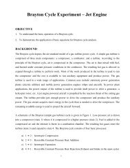
Turb<strong>in</strong>e Eng<strong>in</strong>es<br />
In most cases, with the exception of civil aviation, modern aircraft are powered by turb<strong>in</strong>e<br />
eng<strong>in</strong>es (also called gas turb<strong>in</strong>es). While piston eng<strong>in</strong>es are efficient for low power<br />
applications, their power (or thrust) to weight ratio drops significantly as eng<strong>in</strong>e power<br />
<strong>in</strong>creases. This makes them unsuitable for large aircraft that require high power eng<strong>in</strong>es. Gas<br />
turb<strong>in</strong>e eng<strong>in</strong>es are also used <strong>in</strong> a number of other applications <strong>in</strong>clud<strong>in</strong>g mar<strong>in</strong>e propulsion,<br />
operat<strong>in</strong>g gas pipel<strong>in</strong>e compressors, <strong>and</strong> most notably, the generation of electric power.<br />
The components of a basic gas turb<strong>in</strong>e system are shown <strong>in</strong> Fig. 9. Air enters the eng<strong>in</strong>e<br />
(through an <strong>in</strong>let not shown) <strong>and</strong> passes through a rotat<strong>in</strong>g compressor that raises the air<br />
pressure. Next, the high pressure air enters the combustor where it is mixed with fuel <strong>and</strong><br />
burned without much change <strong>in</strong> pressure. The hot products then pass through a rotat<strong>in</strong>g<br />
turb<strong>in</strong>e that extracts work from the flow <strong>and</strong> sends it to the compressor via a rotat<strong>in</strong>g shaft.<br />
The exhaust of the turb<strong>in</strong>e is a hot, high pressure gas. In a turbojet, the exhaust is exp<strong>and</strong>ed<br />
through a nozzle (Fig. 10), which converts the thermal energy to k<strong>in</strong>etic energy, i.e., it<br />
accelerates the gas <strong>in</strong> order to produce thrust. On the other h<strong>and</strong> <strong>in</strong> a turboshaft eng<strong>in</strong>e, the<br />
hot, high pressure gas exit<strong>in</strong>g the first turb<strong>in</strong>e is exp<strong>and</strong>ed through a follow<strong>in</strong>g power turb<strong>in</strong>e<br />
that converts the thermal energy to shaft power, which can be used to run a rotor <strong>in</strong> a<br />
helicopter eng<strong>in</strong>e or to turn an electric generator <strong>in</strong> an aircraft’s auxiliary power unit (APU) or<br />
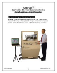
<strong>in</strong> a ground power station. In this lab, you will operate <strong>and</strong> perform measurements on an SR-<br />
30 turbojet manufactured by Turb<strong>in</strong>e Technologies, Ltd. (Fig. 11), operat<strong>in</strong>g on Jet-A fuel.<br />
Thermodynamic Analysis – The follow<strong>in</strong>g is a brief description of the thermodynamic<br />
expressions used to analyze a jet eng<strong>in</strong>e. * The processes that occur <strong>in</strong> a turb<strong>in</strong>e eng<strong>in</strong>e can be<br />
modeled, <strong>in</strong> the ideal case, † by a Brayton cycle. As shown <strong>in</strong> Fig. 12, the ideal compressor<br />
(2→3), turb<strong>in</strong>e (4→5) <strong>and</strong> nozzle (5→e) can be modeled as isentropic processes (constant<br />
entropy, s). The ideal combustor (3→4) is modeled as a constant pressure heat addition, where<br />
the “heat” comes from burn<strong>in</strong>g the fuel, <strong>and</strong> the heat release rate is given by<br />
* A more detailed development can be found <strong>in</strong> the text for AE 4451, Hill <strong>and</strong> Peterson’s Mechanics <strong>and</strong><br />
Thermodynamics of Propulsion.<br />
† Mean<strong>in</strong>g each component of the eng<strong>in</strong>e is reversible <strong>and</strong> has no heat losses.<br />
6
AE 3051<br />
<strong>Temperature</strong> <strong>Measurements</strong> <strong>in</strong> a Jet Eng<strong>in</strong>e<br />
where<br />
Q& = m&<br />
× HV<br />
(3)<br />
f<br />
m&<br />
f<br />
is the fuel mass flow rate <strong>and</strong> HV is the heat<strong>in</strong>g value of the fuel (~45 MJ/kg fuel for<br />
most liquid jet fuels).<br />
For the three isentropic processes, we can f<strong>in</strong>d a relationship between the ratios of<br />
temperature (absolute, i.e., <strong>in</strong> Kelv<strong>in</strong> or Rank<strong>in</strong>e units) <strong>and</strong> pressure (absolute, not gauge<br />
pressure) across each device from the entropy state equation for a perfect gas, i.e., for an<br />
isentropic process go<strong>in</strong>g from state a to state b,<br />
T b cp<br />
dT<br />
∫<br />
T a R T<br />
Tb<br />
dT p p<br />
b b<br />
0 = s − s = ∫ c − Rln<br />
⇒ = e<br />
b a p<br />
T T p p<br />
a<br />
a a<br />
. (4)<br />
Assum<strong>in</strong>g that the gas is also calorically perfect (c p =constant),<br />
p ⎛ T<br />
b<br />
=<br />
⎜<br />
pa<br />
⎝T<br />
or equivalently for stagnation properties,<br />
b<br />
a<br />
⎞<br />
⎟<br />
⎠<br />
cp<br />
R<br />
⎛ T<br />
=<br />
⎜<br />
⎝T<br />
b<br />
a<br />
⎞<br />
⎟<br />
⎠<br />
γ<br />
γ −1<br />
(5a)<br />
where γ is the ratio of specific heats (γ=c p /c v ).<br />
p<br />
p<br />
ob<br />
oa<br />
⎛T<br />
=<br />
⎜<br />
⎝T<br />
ob<br />
oa<br />
⎞<br />
⎟<br />
⎠<br />
γ<br />
γ −1<br />
(5b)<br />
There is also a relationship between the stagnation temperature change across the<br />
compressor <strong>and</strong> turb<strong>in</strong>e. S<strong>in</strong>ce the turb<strong>in</strong>e is used to power the compressor, the output power<br />
of the turb<strong>in</strong>e should equal the power <strong>in</strong>put to the compressor (assum<strong>in</strong>g steady operation <strong>and</strong><br />
no shaft losses, which are typically less than 1% of the shaft power). Therefore from<br />
conservation of energy (<strong>and</strong> for adiabatic conditions),<br />
where<br />
T<br />
( m&<br />
+ m&<br />
) c ( T − T ) = m&<br />
c ( T − T ) W&<br />
a f p T o4<br />
o5<br />
a p,<br />
C o3<br />
o C<br />
W & = =<br />
(6)<br />
, 2<br />
m&<br />
a is air mass flow rate enter<strong>in</strong>g the eng<strong>in</strong>e, <strong>and</strong> c p,T <strong>and</strong> c p,C are the (average) specific<br />
heats of the gases pass<strong>in</strong>g through the turb<strong>in</strong>e <strong>and</strong> compressor. Similarly, the velocity at the<br />
nozzle exit can be found from<br />
u<br />
e<br />
= c<br />
p,<br />
N<br />
( T − T )<br />
2 (7)<br />
where c p,N is the (average) specific heat of the gas pass<strong>in</strong>g through the nozzle, <strong>and</strong> T oe =T 05<br />
(aga<strong>in</strong> assum<strong>in</strong>g the nozzle is adiabatic, i.e. no heat losses). For the combustor, aga<strong>in</strong> us<strong>in</strong>g<br />
oe<br />
e<br />
7
AE 3051<br />
<strong>Temperature</strong> <strong>Measurements</strong> <strong>in</strong> a Jet Eng<strong>in</strong>e<br />
energy conservation, we can calculate the expected change <strong>in</strong> temperature caused by burn<strong>in</strong>g<br />
the fuel:<br />
where f is the fuel-air ratio m & m&<br />
.<br />
( T + f HV c ) ( f )<br />
T = 1+<br />
(8)<br />
o 4 o3<br />
p,<br />
Combustor<br />
f<br />
a<br />
If the compressor, turb<strong>in</strong>e <strong>and</strong> nozzle are not ideal, i.e., they are not reversible (but still<br />
adiabatic), the temperature <strong>and</strong> pressure ratios across each component are related by the<br />
adiabatic component efficiencies: * γ −1<br />
( po3<br />
p<br />
2<br />
) γ<br />
o<br />
−<br />
compressor<br />
=<br />
( T T ) −1<br />
o3<br />
o2<br />
1−<br />
( T )<br />
o5<br />
To<br />
4<br />
ηturb<strong>in</strong>e<br />
=<br />
γ −1<br />
1−<br />
( p )<br />
o5<br />
po4<br />
γ<br />
1−<br />
( T )<br />
e<br />
To<br />
5<br />
η =<br />
nozzle<br />
γ −1<br />
1−<br />
( p p ) γ<br />
1<br />
η (9)<br />
Note, if the nozzle is truly adiabatic, then ( ) γ<br />
e<br />
e<br />
o5<br />
o5<br />
= Te<br />
Toe<br />
= pe<br />
poe<br />
γ −1<br />
T T<br />
.<br />
(10)<br />
(11)<br />
We can also def<strong>in</strong>e an overall thermal efficiency of a static (stationary) turbojet eng<strong>in</strong>e,<br />
which is given by,<br />
( m + m&<br />
)<br />
2<br />
Output K<strong>in</strong>etic Power &<br />
f a<br />
u 2<br />
e<br />
η<br />
th<br />
=<br />
=<br />
. (12)<br />
Input Heat Rate m&<br />
HV<br />
If the turbojet is ideal (<strong>and</strong> c p is assumed constant throughout the eng<strong>in</strong>e), it can be shown that<br />
the thermal efficiency should solely be a function of the cycle pressure ratio:<br />
η = 1−<br />
th<br />
−1<br />
γ<br />
γ<br />
( p p )<br />
3<br />
1<br />
2<br />
f<br />
. (13)<br />
Thus as pressure ratio of the compressor <strong>in</strong>creases, η th of the eng<strong>in</strong>e should <strong>in</strong>crease.<br />
Safety Considerations<br />
As with any combustion experiment safety is a primary concern. Improper operation of<br />
the jet eng<strong>in</strong>e can damage the eng<strong>in</strong>e, <strong>and</strong> pose a hazard to those nearby. Carefully follow all<br />
the safety <strong>in</strong>structions presented dur<strong>in</strong>g the lab concern<strong>in</strong>g startup, operation <strong>and</strong> shutdown of<br />
8
AE 3051<br />
<strong>Temperature</strong> <strong>Measurements</strong> <strong>in</strong> a Jet Eng<strong>in</strong>e<br />
the eng<strong>in</strong>e. Do not operate the eng<strong>in</strong>e without direct supervision by the lab technician. Do not<br />
place any part of your body, or any objects <strong>in</strong> the <strong>in</strong>let or exhaust regions. All students<br />
work<strong>in</strong>g <strong>in</strong> the lab MUST WEAR safety glasses/goggles <strong>in</strong> the lab <strong>and</strong> hear<strong>in</strong>g protection<br />
when the eng<strong>in</strong>e is operat<strong>in</strong>g (both will be supplied to you).<br />
Prelim<strong>in</strong>ary<br />
The follow<strong>in</strong>g items must be turned <strong>in</strong> at the start of your lab session.<br />
1. Us<strong>in</strong>g the <strong>in</strong>formation supplied <strong>in</strong> Table 2, determ<strong>in</strong>e the thermocouple voltage you would<br />
expect to measure if the type-K thermocouple junction was at room temperature (~74°F)<br />
<strong>and</strong> the reference junction was placed <strong>in</strong> an ice bath.<br />
2. Br<strong>in</strong>g a modified copy of the equation you developed <strong>in</strong> the earlier labs that relates<br />
dynamic pressure to velocity of a gas, <strong>and</strong> the ambient pressure <strong>and</strong> temperature. You need<br />
to modify the equation to use dynamic pressure <strong>in</strong> psi rather than mm Hg.<br />
Procedure<br />
1. Locate the electronic barometer/thermometer <strong>and</strong> record the ambient pressure <strong>and</strong><br />
temperature.<br />
2. Locate the type K, unshielded thermocouple probe (it has a yellow base). Connect the<br />
probe to the color-coded type K thermocouple extension wire. Then connect the extension<br />
wires to the st<strong>and</strong>ard electrical wire us<strong>in</strong>g the strip screw term<strong>in</strong>al accord<strong>in</strong>g to the<br />
diagram of Fig. 14. Record the thermocouple voltage with the thermocouple exposed to<br />
the ambient air, <strong>and</strong> any other systems you can measure (e.g., an ice bath or boil<strong>in</strong>g water).<br />
3. Aga<strong>in</strong> record the thermocouple voltage with the thermocouple exposed to the ambient air,<br />
except this time raise <strong>and</strong> lower the temperature of the screw term<strong>in</strong>al junctions. You<br />
should do this: a) where the thermocouple extension wires connect to the first set of<br />
electrical wires <strong>and</strong> b) aga<strong>in</strong> where the first <strong>and</strong> second set of electrical wires are<br />
connected. You can also try to change the temperature of a s<strong>in</strong>gle connector or both<br />
connectors <strong>in</strong> each junction. Record the measured voltage for each of these various cases.<br />
4. Disconnect the extension wires from the probe, <strong>and</strong> connect the probe to the electronic ice<br />
po<strong>in</strong>t module (small rectangular yellow box). Connect the module to the voltmeter, <strong>and</strong><br />
switch on the ice po<strong>in</strong>t module (be careful not to rotate the switch all the way to the ON<br />
* The efficiency compares an actual process to an isentropic one that has the same start<strong>in</strong>g condition <strong>and</strong> same pressure ratio.<br />
9
AE 3051<br />
<strong>Temperature</strong> <strong>Measurements</strong> <strong>in</strong> a Jet Eng<strong>in</strong>e<br />
mark; make sure the voltage read<strong>in</strong>g changes after you turn the module on). Record the<br />
thermocouple voltage with the thermocouple exposed to the ambient air <strong>and</strong> any other<br />
systems you wish.<br />
5. Turn off the ice po<strong>in</strong>t module.<br />
6. Take a tour of the turboshaft eng<strong>in</strong>e cutaway <strong>in</strong> the Combustion Lab foyer.<br />
7. Familiarize yourself with the flowpath through the SR-30 turbojet eng<strong>in</strong>e.<br />
8. Review the safety, startup, <strong>and</strong> eng<strong>in</strong>e shutdown procedures with the lab TA’s <strong>and</strong> with<br />
the lab technician who will oversee the eng<strong>in</strong>e operation.<br />
9. Determ<strong>in</strong>e the cross-sectional area of the flow where the <strong>in</strong>let velocity is measured.<br />
10. Ask the lab technician to start the eng<strong>in</strong>e (the technician may ask students to help, but the<br />
eng<strong>in</strong>e should be started only under the supervision of the lab technician).<br />
11. Acquire data for at least 5 RPM conditions (change RPM by chang<strong>in</strong>g the throttle – which<br />
changes the fuel flowrate). DO NOT EXCEED 82,000 RPM. The data acquisition program<br />
will allow you to cont<strong>in</strong>uously monitor the eng<strong>in</strong>e RPM, pressures <strong>and</strong> temperatures.<br />
When you decide to acquire data at some RPM, the software will sample all the probes,<br />
<strong>and</strong> update graphs of eng<strong>in</strong>e conditions vs. RPM. Each time you acquire the data, the<br />
computer will pause until you are ready to return to the real-time display. NOTE: it will<br />
be very hard to hear while the eng<strong>in</strong>e is runn<strong>in</strong>g. Make sure your group has discussed what<br />
conditions you are look<strong>in</strong>g for <strong>and</strong> work out some h<strong>and</strong> signals to identify when you want<br />
to take data <strong>and</strong> when you want to return to the real-time display.<br />
12. When you are f<strong>in</strong>ished, ask the technician to shutdown the eng<strong>in</strong>e.<br />
Data to be Taken<br />
1. Ambient pressure <strong>and</strong> temperature.<br />
2. Voltages from the type-K thermocouple probe connected to the voltmeter under the<br />
different connection <strong>and</strong> temperature cases described above.<br />
3. Cross-sectional area of the compressor <strong>in</strong>let.<br />
4. Values of: 1) dynamic pressure <strong>and</strong> T 2 at the compressor <strong>in</strong>let, 2) T o3 <strong>and</strong> p o3 (gauge) at the<br />
compressor exit, 3) p o4 (gauge) <strong>and</strong> T o4 at the turb<strong>in</strong>e <strong>in</strong>let, 4) p o5 (gauge) <strong>and</strong> T o5 at the<br />
turb<strong>in</strong>e exit, 5) p o6 (gauge) <strong>and</strong> ~T o6 at the nozzle exit, <strong>and</strong> 6) pressure drop (a voltage<br />
signal) <strong>in</strong> the fuel system at various RPM sett<strong>in</strong>gs.<br />
10
AE 3051<br />
<strong>Temperature</strong> <strong>Measurements</strong> <strong>in</strong> a Jet Eng<strong>in</strong>e<br />
Data Reduction<br />
1. Unshielded thermocouple probe temperatures reduced from the measured voltages<br />
(without heat<strong>in</strong>g or cool<strong>in</strong>g the strip term<strong>in</strong>al junctions).<br />
2. Air mass flowrate (from dynamic pressure at the compressor <strong>in</strong>let).<br />
3. Fuel mass flowrate (from fuel pressure read<strong>in</strong>g <strong>and</strong> calibration, see Table 3).<br />
4. Compressor efficiency.<br />
5. Exit static temperature determ<strong>in</strong>ed from the nozzle exit p o6 (which is measured as a gauge<br />
pressure here) <strong>and</strong> the exit stagnation temperature T oe .<br />
6. Nozzle exit velocity.<br />
7. An estimate of the heat loss rate from gas to the nozzle (based on the difference <strong>in</strong><br />
stagnation temperature across the nozzle).<br />
8. Compressor <strong>and</strong> turb<strong>in</strong>e powers (assum<strong>in</strong>g adiabatic operation).<br />
9. The actual eng<strong>in</strong>e thermal efficiency.<br />
Results Needed for Report<br />
1. Tables of the thermocouple voltages <strong>and</strong> reduced temperatures for the different cases.<br />
2. Tables of the raw <strong>and</strong> reduced eng<strong>in</strong>e conditions at each operat<strong>in</strong>g RPM.<br />
3. Plot of the compressor pressure ratio versus air mass flowrate.<br />
4. Plot of the compressor efficiency versus air mass flowrate.<br />
5. Plot of the heat loss <strong>in</strong> the nozzle rate versus air mass flowrate.<br />
6. Plot of the eng<strong>in</strong>e thermal efficiency versus compressor pressure ratio.<br />
Further Read<strong>in</strong>g<br />
1. Philip Hill <strong>and</strong> Carl Peterson, Mechanics <strong>and</strong> Thermodynamics of Propulsion, 2 nd edition,<br />
Prentice-Hall, 1992.<br />
11
AE 3051<br />
<strong>Temperature</strong> <strong>Measurements</strong> <strong>in</strong> a Jet Eng<strong>in</strong>e<br />
Table 1. Some st<strong>and</strong>ard thermocouple materials <strong>and</strong> their properties.<br />
T<br />
Material<br />
max ANSI Allowable<br />
°C (°F) Type atmosphere<br />
Avg Output<br />
mV/100°C<br />
Tungsten/<br />
tungsten 26% rhenium<br />
2320/4210 - <strong>in</strong>ert, H 2 (nonoxidiz<strong>in</strong>g) 1.7<br />
Tungsten 5% rhenium/<br />
tungsten 26% rhenium<br />
2320/4210 - <strong>in</strong>ert, H 2 (nonoxidiz<strong>in</strong>g) 1.6<br />
Plat<strong>in</strong>um 30% rhodium/<br />
plat<strong>in</strong>um 6% rhodium<br />
1820/3310 B oxidiz<strong>in</strong>g, <strong>in</strong>ert 0.76<br />
Plat<strong>in</strong>um 13% rhodium/<br />
plat<strong>in</strong>um<br />
1770/3200 R oxidiz<strong>in</strong>g, <strong>in</strong>ert 1.2<br />
Plat<strong>in</strong>um 10% rhodium/<br />
plat<strong>in</strong>um<br />
1770/3200 S oxidiz<strong>in</strong>g, <strong>in</strong>ert 1.0<br />
Chromel/alumel 1370/2500 K oxidiz<strong>in</strong>g, <strong>in</strong>ert * 3.9<br />
Chromel/constantan 1000/1830 E oxidiz<strong>in</strong>g, <strong>in</strong>ert * 6.8<br />
Iron/constantan 1200/2193 J reduc<strong>in</strong>g, <strong>in</strong>ert, vacuum † 5.5<br />
Copper/constantan 400/750 T<br />
mild oxidiz<strong>in</strong>g, reduc<strong>in</strong>g<br />
vacuum, <strong>in</strong>ert<br />
4.0<br />
* Limited use <strong>in</strong> vacuum or reduc<strong>in</strong>g environments<br />
† Limited use <strong>in</strong> oxidiz<strong>in</strong>g at high temperature<br />
Table 2. ITS-90 thermocouple <strong>in</strong>verse polynomials for type K thermocouples; two<br />
polynomial fits are listed, for separate temperature/voltage ranges. The reference junction<br />
i<br />
is assumed to be at 0°C, <strong>and</strong> the polynomials are of the form, T = ∑ a i<br />
V , with T <strong>in</strong><br />
degrees Celsius <strong>and</strong> V <strong>in</strong> microvolts.<br />
<strong>Temperature</strong> Range 0-500 °C 500-1372 °C<br />
Voltage Range 0-20,644 μV 20,644-54,886 μV<br />
a 0 0.000000 -1.318058×10 2<br />
a 1 2.508355×10 -2 4.830222×10 -2<br />
a 2 7.860106×10 -8 -1.646031×10 -06<br />
a 3 -2.503131×10 -10 5.464731×10 -11<br />
a 4 8.315270×10 -14 -9.650715×10 -16<br />
a 5 -1.228034×10 -17 8.802193×10 -21<br />
a 6 9.804036×10 -22 -3.110810×10 -26<br />
a 7 -4.413030×10 -26<br />
a 8 1.057734×10 -30<br />
a 9 -1.052755×10 -35<br />
Table 3. Calibration data for fuel flowrate.<br />
Voltage (Volts) Flowrate (cc/m<strong>in</strong>)<br />
1.7 175<br />
2.2 227<br />
2.8 255<br />
3.0 300<br />
12
AE 3051<br />
<strong>Temperature</strong> <strong>Measurements</strong> <strong>in</strong> a Jet Eng<strong>in</strong>e<br />
Metal A<br />
Metal A<br />
V<br />
0 L<br />
T cold<br />
junction<br />
T hot<br />
junction<br />
Metal B<br />
Figure 1. Simple (open) thermoelectric thermocouple circuit.<br />
A<br />
3<br />
V th<br />
1<br />
2<br />
sensor<br />
junction<br />
reference<br />
junction<br />
B<br />
Figure 2. Ideal thermoelectric circuit, with the thermocouple voltage measured across the<br />
isothermal reference junction.<br />
Junction <strong>Temperature</strong> (°C)<br />
1500<br />
1000<br />
500<br />
0<br />
0 10 20 30 40 50<br />
Thermocouple Voltage (mV)<br />
Type K<br />
Figure 3. Sensitivity of a st<strong>and</strong>ard type-K thermocouple, based on ITS-90 <strong>in</strong>verse<br />
polynomial fit. The millivolt output is based on a reference temperature of 0°C.<br />
13
AE 3051<br />
<strong>Temperature</strong> <strong>Measurements</strong> <strong>in</strong> a Jet Eng<strong>in</strong>e<br />
Chromel<br />
+<br />
V<br />
Iron<br />
Copper<br />
Pt-Rhodium<br />
T<br />
Alumel<br />
−<br />
Constantan<br />
Figure 4. Voltage−temperature response for several metals.<br />
V<br />
3<br />
Constantan<br />
V th<br />
1<br />
T ref<br />
2<br />
T probe,1<br />
Iron<br />
T<br />
T probe,2<br />
Figure 5. Development of the voltage difference across the thermocouple, V th , <strong>in</strong> a<br />
thermocouple circuit, like that of Fig. 2, formed by two metals.<br />
5<br />
V th<br />
1<br />
device<br />
junction<br />
Copper<br />
Copper<br />
4<br />
2<br />
reference<br />
junction<br />
Constantan<br />
Iron<br />
3<br />
sensor<br />
junction<br />
Figure 6. Modified circuit; copper extension wires connect the thermocouple to the<br />
measur<strong>in</strong>g device, <strong>and</strong> the device connections are at the same temperature.<br />
14
AE 3051<br />
<strong>Temperature</strong> <strong>Measurements</strong> <strong>in</strong> a Jet Eng<strong>in</strong>e<br />
ΔV Cu<br />
V<br />
4<br />
5<br />
Copper<br />
V 15<br />
V th =<br />
V 24<br />
Constantan<br />
3<br />
2<br />
1<br />
Iron<br />
T<br />
ΔV Cu<br />
T ref<br />
T device<br />
T probe<br />
Figure 7. Development of the thermocouple voltage difference for the thermocouple<br />
circuit shown <strong>in</strong> Fig. 6. If the wires connect<strong>in</strong>g po<strong>in</strong>ts 1 to 2, <strong>and</strong> 4 to 5 are identical, <strong>and</strong><br />
the temperatures T 1 <strong>and</strong> T 5 are the same, then the voltage measured across the device<br />
(V 15 ) is equal to the voltage that would be produced by the ideal thermocouple circuit<br />
(V th =V 24 ).<br />
probe body<br />
Unshielded<br />
Probe<br />
<strong>in</strong>sulation<br />
Shielded<br />
Probe<br />
flow<br />
Shielded<br />
Stagnation<br />
Probe<br />
Figure 8. Examples of unshielded, shielded <strong>and</strong> stagnation thermocouple probes.<br />
Compressor<br />
Combustor<br />
Air<br />
Fuel<br />
Shaft<br />
Turb<strong>in</strong>e<br />
Hot, High<br />
<strong>Pressure</strong> Gas<br />
Figure 9. Basic components of a gas turb<strong>in</strong>e eng<strong>in</strong>e.<br />
15
AE 3051<br />
<strong>Temperature</strong> <strong>Measurements</strong> <strong>in</strong> a Jet Eng<strong>in</strong>e<br />
Compressor<br />
Combustor<br />
Air<br />
Shaft<br />
Fast, Warm, Atm.<br />
Press. Gas<br />
Fuel Turb<strong>in</strong>e<br />
2<br />
3<br />
4 5 e<br />
Figure 10. Basic components of a gas turb<strong>in</strong>e eng<strong>in</strong>e.<br />
Figure 11. Schematic of the gas turb<strong>in</strong>e system to be used <strong>in</strong> this lab.<br />
16
AE 3051<br />
<strong>Temperature</strong> <strong>Measurements</strong> <strong>in</strong> a Jet Eng<strong>in</strong>e<br />
4<br />
T<br />
3<br />
5<br />
2<br />
e<br />
Figure 12. Ideal Brayton cycle; stations 2-e correspond to the number<strong>in</strong>g scheme shown<br />
<strong>in</strong> Fig. 10.<br />
s<br />
4<br />
T<br />
3<br />
5<br />
e<br />
2<br />
Figure 13. Turbojet cycle with nonideal components.<br />
s<br />
elec. wire<br />
elec. wire<br />
K (+)<br />
voltmeter<br />
elec. wire<br />
strip<br />
term<strong>in</strong>al<br />
elec. wire<br />
strip<br />
term<strong>in</strong>al<br />
Figure 14. Thermocouple circuit to be used <strong>in</strong> this lab.<br />
K (-)<br />
sensor<br />
junction<br />
17