Econometrics I ab exercises-Chapter 5 Exercises on endogeneity ...
Econometrics I ab exercises-Chapter 5 Exercises on endogeneity ...
Econometrics I ab exercises-Chapter 5 Exercises on endogeneity ...
Create successful ePaper yourself
Turn your PDF publications into a flip-book with our unique Google optimized e-Paper software.
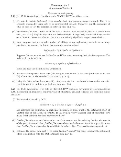
<str<strong>on</strong>g>Ec<strong>on</strong>ometrics</str<strong>on</strong>g> I<br />
<str<strong>on</strong>g>ab</str<strong>on</strong>g> <str<strong>on</strong>g>exercises</str<strong>on</strong>g>-<str<strong>on</strong>g>Chapter</str<strong>on</strong>g> 5<br />
<str<strong>on</strong>g>Exercises</str<strong>on</strong>g> <strong>on</strong> <strong>endogeneity</strong><br />
5.1) (Ex. 15.12 Wooldridge). Use the data in WAGE2.RAW for this exercise:<br />
(i) We want to explain log(wage) based <strong>on</strong> educ, but educ is an endogenous vari<str<strong>on</strong>g>ab</str<strong>on</strong>g>le. Use IV to<br />
estimate this model, using sibs as an instrumental vari<str<strong>on</strong>g>ab</str<strong>on</strong>g>le. Moreover, run the regressi<strong>on</strong> of<br />
educ <strong>on</strong> sibs to test the correlati<strong>on</strong> between educ and sibs.<br />
(ii) The vari<str<strong>on</strong>g>ab</str<strong>on</strong>g>le brthord is birth order (brthord is <strong>on</strong>e for a first-born child, two for a sec<strong>on</strong>d-born<br />
child, and so <strong>on</strong>). Explain why educ and brthord might be negatively correlated. Regress educ<br />
<strong>on</strong> brthord to determine whether there is a statistically significant negative correlati<strong>on</strong>.<br />
(iii) Now, suppose that we include number of siblings as an explanatory vari<str<strong>on</strong>g>ab</str<strong>on</strong>g>le in the wage<br />
equati<strong>on</strong>; this c<strong>on</strong>trols for family background, to some extent<br />
log(wage) = β 0 + β 1 educ + β 2 sibs + u.<br />
Suppose that we want to use brthord as an IV for educ, assuming that sibs is exogenous. The<br />
reduced form for educ is:<br />
State and test the identificati<strong>on</strong> assumpti<strong>on</strong>.<br />
educ = π 0 + π 1 sibs + π 2 brthord + v.<br />
(iv) Estimate the equati<strong>on</strong> from part (iii) using brthord as an IV for educ (and sibs as its own<br />
IV). Comment <strong>on</strong> the standard errors for β 1 y de β 2 .<br />
(v) Using the fitted values from part (iii), educ, ˆ compute the correlati<strong>on</strong> between<br />
Use this result to explain your findings from part (iv).<br />
ˆ educ and sibs.<br />
5.2) (Ex. 15.13 Wooldridge) The data in FERTIL2.RAW includes, for women in Botswana during<br />
1988, informati<strong>on</strong> <strong>on</strong> number of children, years of educati<strong>on</strong>, age, and religious and ec<strong>on</strong>omic status<br />
vari<str<strong>on</strong>g>ab</str<strong>on</strong>g>les.<br />
(i) Estimate this model by OLS<br />
children = β 0 + β 1 educ + β 2 age + β 3 age 2 + u<br />
and interpret the estimates. In particular, holding age fixed, what is the estimated effect of<br />
another year of educati<strong>on</strong> <strong>on</strong> fertility If 100 women receive another year of educati<strong>on</strong>, how<br />
many fewer children are they expected to have<br />
(ii) frsthalf is a dummy vari<str<strong>on</strong>g>ab</str<strong>on</strong>g>le equal to <strong>on</strong>e if the woman was born during the first six m<strong>on</strong>ths<br />
of the year. Assuming that frsthalf is uncorrelated with the error term from part (i), show<br />
that frsthalf is a reas<strong>on</strong><str<strong>on</strong>g>ab</str<strong>on</strong>g>le IV candidate for educ. (Hint: You need to do a regressi<strong>on</strong>.)<br />
(iii) Estimate the model from part (i) by using frsthalf as an IV for educ. Compare the estimated<br />
effect of educati<strong>on</strong> with the OLS estimate from part (i).<br />
1
(iv) Add the binary vari<str<strong>on</strong>g>ab</str<strong>on</strong>g>les electric, tv, and bicycle to the model and assume these are exogenous.<br />
Estimate the equati<strong>on</strong> by OLS and 2SLS and compare the estimated coefficients<br />
<strong>on</strong> educ. Interpret the coefficient <strong>on</strong> tv and explain why televisi<strong>on</strong> ownership has a negative<br />
effect <strong>on</strong> fertility.<br />
5.3). The aim of this exercise is to compare the estimati<strong>on</strong>s obtained with 2SLS with others obtained<br />
by incorrect methods. The data is WAGE2.<br />
(i) Use 2SLS to estimate:<br />
log(wage) = β 0 + β 1 educ + β 2 exper + β 3 tenure + β 4 black + u,<br />
using sibs as instrumental vari<str<strong>on</strong>g>ab</str<strong>on</strong>g>le for educ.<br />
(ii) Estimate now the reressi<strong>on</strong> of educ <strong>on</strong> sibs, exper, tenure and black. Then plug in educ ˆ in<br />
the equati<strong>on</strong> of part (i) and estimate it by OLS. Compare these ˆβ j with the <strong>on</strong>es obtained in<br />
part (i) and their standard errors. Comment these standard errors.<br />
2


