Using the SAS System to Fit the Burr XII Distribution to Lifetime Data ...

Using the SAS ® System to Fit the Burr XII Distribution to
Lifetime Data
A J Watkins, University of Wales Swansea
Introduction
This paper is concerned with various practical and theoretical aspects of using the
Burr XII distribution to model lifetime data, and thus indicates some possible
additional features and refinements to the SAS/STAT ® procedure LIFEREG. Despite
its lengthy pedigree, having been introduced by Burr (1942), the Burr XII distribution
has remained rather neglected as an option in the analysis of lifetime data. However,
there are recent indications that this distribution possesses sufficient flexibility to
make it a possible model for various types of data; for instance, it has been used to
model business failure data (Lomax, 1954), the efficacy of analgesics in clinical trials
(Wingo, 1983), and the times to failure of electronic components (Wang, Keats and
Zimmer, 1996).
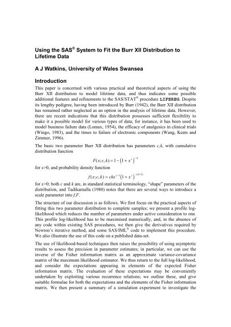
The basic two parameter Burr XII distribution has parameters c,k, with cumulative
distribution function
( )
F x c k x c −k
( ; , ) = 1 − 1 +
for x>0, and probability density function
( 1 )
c − 1 c − ( k + 1)
f ( x; c, k)
= ckx + x
for x>0; both c and k are, in standard statistical terminology, “shape” parameters of the
distribution, and Tadikamalla (1980) notes that there are several ways to introduce a
scale parameter into f,F.
The structure of our discussion is as follows. We first focus on the practical aspects of
fitting this two parameter distribution to complete samples; we present a profile loglikelihood
which reduces the number of parameters under active consideration to one.
This profile log-likelihood has to be maximised numerically, and, in the absence of
any code within existing SAS procedures, we then give the derivatives required by
Newton’s iterative method, and some SAS/IML ® code to implement this procedure.
We also illustrate the use of this code on a published data-set.
The use of likelihood-based techniques then raises the possibility of using asymptotic
results to assess the precision in parameter estimates; in particular, we can use the
inverse of the Fisher information matrix as an approximate variance-covariance
matrix of the maximum likelihood estimator. We thus return to the full log-likelihood,
and consider the expectations appearing in elements of the expected Fisher
information matrix. The evaluation of these expectations may be conveniently
undertaken by exploiting various recurrence relations; we outline these, and give
suitable formulae for both the expectations and the elements of the Fisher information
matrix. We then present a summary of a simulation experiment to investigate the

agreement between these asymptotically valid formulae and the results obtained in
practice with samples of small to moderate size.
Full and Profile Log-Likelihoods
We assume that the data for analysis is X 1 ,X 2 ,...,X n , comprising the times to failure of
n items, so that the log-likelihood is
n
∑ ∑ ∑
( c
i )
l = log f ( X ; c, k) = n log( ck) + ( c − 1) log X − ( k + 1) log 1 + X ,
i
i
i= 1 i= 1 i=
1
here, as throughout the paper, we use natural (or base e) logarithms. The partial
derivative of l with respect to c requires
so that we have
together with
Solving
∂l
∂
d
dc
⎡
⎢
⎣
n
( X
c
i
∑ log 1 +
i ) ∑ ,
c
i= 1 = 1
n
n c
⎤ Xi
log X
⎥
⎦
= i 1 + Xi
n
∂l
−1
= nc + ∑ log Xi
− ( k + 1)
∂c
i= 1 i=
1
n
∑
n
∂l
−1
c
= nk − ∑ log ( 1 + X i ) .
∂k
i=
1
k = 0 for k in terms of c yields ~ n
k =
n
c
log( + X i )
∑ 1
i=
1
,
c
Xi
log X
1 + X
so that we may derive a profile log-likelihood l * by substituting ~ k in l, and then
simplifying. We obtain
n
n
n
*
c
l = n log( c) + ( c − 1 ) log Xi
− log( + Xi
) − n log ⎡
⎤
∑ ∑ 1 ⎢∑
log( + X
c
i ) ⎥
i= i=
⎣
1
1 1
i=
1
⎦
and can now maximise l * with respect to c. This remains a numerical exercise, and
options for finding the maximising value of c include those based on the first and
second derivatives of l * . From the above discussion, we have
*
dl
dc
n
∑
−1
= nc + log X −
i=
1
i
n
∑
X
c
i
i=
1 1
log X
+ X
c
i
i
⎡
⎢
− n⎢
⎢
⎢
⎣
n
∑
i=
1
n
∑
i=
1
X
c
i
log
c
i
i
n
log X
1 + X
c
i
( 1 + X
c
i )
i
⎤
⎥
⎥.
⎥
⎥
⎦
We next note that
d
dc
n c
c
2
n
X X X ( X
i
log
i
⎤
i
log
i )
∑ c ∑ ,
c 2
⎡
⎢
⎣
⎥
1 + X
= i ⎦ i 1 ( 1 + Xi
)
i= 1
=

so that the second derivative of l * is
nc
−2
−
n
∑
i=
1
X
c
i
( log X )
1 + X
c
i
i
2
⎡⎧
⎢⎨
⎢⎩
− n⎢
⎢
⎢
⎣⎢
n
c
2
n
X ( X
n
⎫⎧
)
X
c ⎪ i
log ⎫
i ⎪ ⎛
∑ log( 1 +
i
) ⎬⎨∑ c 2 ⎬ ⎜∑
c
Xi
Xi
c
⎭ i Xi
i
⎩⎪ +
⎭⎪ − log ⎞
⎟
1 ( 1 ) ⎝ 1 1 + Xi
⎠
i= 1
= =
⎧
⎨
⎩
n
∑
i=
1
c ⎫
log( 1 + Xi
) ⎬
⎭
2
2
⎤
⎥
⎥
⎥.
⎥
⎥
⎦⎥
The following SAS/IML code, loosely based on that given in Example 2 in the
available documentation (SAS Institute, 1989), implements the standard Newton
iterative method for finding the maximising value of c: the corresponding value of k is
then found by calculating ~ k at this maximising value of c.
proc iml;
/* structure based on example 2 in SAS/IML manual pp113-114 */
start newton;
run fun;
do iter=1 to 10
while(max(abs(plc))>0.0001);
c = c - solve(plcc,plc);
run fun;
end;
finish newton;
/* fun gives profile log-likelihood and first two derivatives */
start fun;
dc = exp(c*c1);
s2 = sum(log(dc+1));
s3 = sum(dc#c1/(dc+1));
s4 = sum(dc#c1#c1/((dc+1)#(dc+1)));
pl = n*log(c) + (c-1)*s1 - s2 - n*log(s2);
plc = n/c + s1 - s3 - n*s3/s2;
plcc = -n/(c*c) - s4 - n*(s2*s4-s3*s3)/(s2*s2);
finish fun;
/* data from Wingo (1983) included explicitly */
do;
data = {0.70, 0.84, 0.58, 0.50, 0.55, 0.82, 0.59, 0.71, 0.72, 0.61,
0.62, 0.49, 0.54, 0.72, 0.36, 0.71, 0.35, 0.64, 0.85, 0.55,
0.59, 0.29, 0.75, 0.53, 0.46, 0.60, 0.60, 0.36, 0.52, 0.68,
0.80, 0.55, 0.84, 0.70, 0.34, 0.70, 0.49, 0.56, 0.71, 0.61,
0.57, 0.73, 0.75, 0.58, 0.44, 0.81, 0.80, 0.87, 0.29, 0.50};
c = 1.0;
n = nrow(data);
c1 = log(data);
s1 = sum(c1);
run newton;
k = n/s2;
print c k plc plcc;
end;
For illustration, the example code contains an explicit listing of data given in Wingo
(1983); in practice, the data may be read from an external file; in simulation
experiments, the data may be generated by further lines of code. The above output

gives the maximising value of c as 5.0006407, with a corresponding value of k as
8.2680792; these values are consistent with those reported both by Wingo (1983) and
Wang, Keats and Zimmer (1996).
The Observed Fisher Information
The first order partial derivatives of the log-likelihood are given above; we now give
the second order counterparts. These are the deterministic quantity
together with
and
2
∂ l
∂c
2
∂ l
∂k
n
= − ,
k
2 2
2 2 n c
∂ l ∂ l Xi
Xi
= = − ∑ log c
∂k∂c
∂c∂k
+ X
,
n
= − − k + 1
c
2 2
i=
1 1
n
( )∑
i=
1
X
c
i ( log Xi
)
2
( 1 + X
c
i )
Expectations for Regularity
It is of some interest to establish regularity of the log-likelihood for complete samples
from the Burr XII distribution by taking expectations of the first and second order
partial derivatives of the full log-likelihood. Reference to these derivatives shows that
we need the expectations of
c
c
c X log X X
log X, log ( 1 + X ),
,
c
1 + X 1 +
i
2
.
( log X)
c
( X )
There are two basic results: the first is that Y=1+X c follows a Pareto distribution with
probability density function ky − ( k+
1) for y>1, so that logY has a negative exponential
distribution with mean k -1 . Thus, we immediately have
The second basic result is
c
[ log( 1 )]
1
E + X = k
− .
r c
[ ] =
Γ( k)
E X
r r
Γ
⎛
⎜ + 1
⎞
⎟Γ
⎛
k −
⎞
⎜ ⎟
⎝ ⎠ ⎝ c⎠
,
where Γ is the usual gamma function. Differentiating this expression with respect to
r, we obtain
2
2

[ r c c
log X] =
cΓ( k)
E X
r r r
Γ
⎛
⎜ + 1
⎞
⎟Γ ⎛
⎜k
−
⎞
⎝ ⎠ ⎝ ⎠
⎟ − Γ
⎛
⎜
⎝ c
+ 1
⎞
⎟Γ
⎠
( 1) ( 1)
⎛ r
k −
⎞
⎜ ⎟
⎝ c⎠
,
where Γ (1) denotes the first derivative of the gamma function. Evaluating this
expectation at r=0 gives
E
[ log X]
( ) ( k) − ( ) ( k)
cΓ( k)
( 1) ( 1)
Γ 1 Γ Γ 1 Γ
+ ( k)
=
= −
⎡γ
Ψ ⎤
⎣⎢ c ⎦⎥
where Ψ = Γ ( 1) / Γ is the digamma or psi function, and γ is Euler’s constant. This
gives the second of the required expectations. However, it should also be noted that
we can obtain the third expectation by an appropriate manipulation of the last result.
Writing expectation as E k to emphasise the role of the parameter k in the Burr XII
distribution, the third expectation is
E X c
⎡ log X ⎤
log X
k
k ⎢
E X E
⎣ X + ⎦
⎥ = − ⎡ ⎤
1 ⎣⎢ X + 1⎦⎥ = − k + 1
[ log ] E [ log X] E [ log X]
c k k c k k+
1
,
on exploiting the form of the probability density function of the Burr XII distribution.
This gives us an expression for the third expectation in terms of Ψ at k and k+1;
further simplification is possible on recalling the recurrence relation
and we thus obtain
Ψ( k + 1) = Ψ( k)
+ k
−
1 ,
E X c
⎡ log X ⎤ ( k)
k ⎢
.
c
X +
⎥
⎣ ⎦
= 1 − γ − Ψ
1 ( k + 1)
c
A similar procedure may also be used to obtain the final expectation from a suitable
expression for
Differentiating E[ X X]
2
[ ]
r
for E X ( log X)
E
[( log
2
X)
]
.
r log with respect to r leads to an expression
2
[ ]
, which, evaluated at r=0, yields E ( log X)
2
⎡π
( 2) ( 1) ( 1) ( 2)
Γ 1 Γ 2Γ 1 Γ Γ 1 Γ
⎢
6
=
⎣
( ) ( k) − ( ) ( k) + ( ) ( k)
2
c Γ( k)
as
2 2 ( 1) ⎤
+ γ + 2γΨ( k) + ( Ψ( k) ) + Ψ ( k)
⎥
⎦
,
2
c
where Γ ( 2)
is the second derivative of the gamma function, Ψ (1) is the derivative of
the digamma function (and is also known as the trigamma function), and
( 2) 2 ( 1)
Γ = Γ × Ψ + Ψ .
( )

⎡
We then write the final expectation as E X c
log
⎢
X
k
c
⎢
⎣ ( 1 + X )
E
k c k
( )
2 2
⎡( log X) ⎤ ⎡ ( log X)
⎤
k
⎢ ⎥ − E ⎢ ⎥ E
X
c 2 k 1
⎣⎢
1 + ⎥⎦
⎢( 1 + X ) ⎥ = −
k + 1 k + 2
⎣ ⎦
2
2
⎤
⎥ , which in turn becomes
⎥
⎦
2 k
[( log X)
] Ek
2 ( log X)
2
[ ]
+ +
,
again by exploiting the form of the probability density function of the Burr XII
(1)
distribution, thus yielding an expression for the expectation in terms of Ψ,
Ψ at k+1
and k+2; further simplification is again possible, since we now also have
Ψ
We obtain the required expectation as
( )
( k + 2) = Ψ ( k + 1)
− k + 1
− .
( 1) ( 1) 2
2
⎡π
2 2 ( 1) ⎤
k⎢
+ γ − 2γ + 2( γ − 1) Ψ( k + 1) + { Ψ( k + 1) } + Ψ ( k + 1)
⎣ 6
⎥
⎦
.
2
( k + 1)( k + 2)
c
Regularity and the Expected Fisher Information
We therefore have
⎡ ∂
E
l ⎤ n
c n n
nE[ X ]
⎣
⎢∂k
⎦
⎥ = k
− log( 1 + ) = k
− k
= 0
and
E
l n
nE[ X ] n k E X c
⎡ ∂ ⎤
X
c
c
⎣
⎢∂c⎦
⎥ = c
+ − + ⎡ log ⎤
log ) ( 1)
⎢
⎣ 1 + X
⎥
⎦
n n{ γ + Ψ( k) } n( k + 1) { 1 − γ − Ψ( k)
}
= −
−
= 0,
c c
( k + 1)
c
after some simplification; these results are as we require. For the expected Fisher
information, we have
2
⎡ ∂ l ⎤ n
E⎢
2 2
⎣∂k
⎥
⎦
= − k
,
2
l
{ }
E nE X c
⎡ ∂ ⎤
X n 1 γ k
⎢
c
∂k∂c
⎥
⎣ ⎦
= − ⎡ log ⎤
⎢
⎣ 1 + X
⎥
⎦
= − − − Ψ( )
( k + 1)
c
and
2
l n
( )
E
n k E X c
X
2
⎡∂
⎤
⎡
⎢ 2 2
∂c
⎥ 1
c
c 2
⎣ ⎦
= − − + log ⎤
( ) ⎢ ⎥
⎢
⎣ ( 1 + X ) ⎥
⎦
2
n ⎡ k ⎧π
2 2 ( 1) ⎫⎤
= − ⎢1
+ ⎨ + γ − 2γ + 2( γ − 1) Ψ( k + 1) + [ Ψ( k + 1) ] + Ψ ( k + 1) 2
⎬⎥.
c ⎣ k + 2 ⎩ 6
⎭⎦
The elements of the inverse of the expected Fisher information matrix can now be
written down; however, there is little or no simplification, and so they are omitted

here. We note that, despite their rather inelegant form, these elements are readily
calculated, although we need to use numerical procedures to calculate Ψ,
Ψ
(1) ; the
former is directly available within SAS via the DIGAMMA function, while the latter
can be evaluated by using an approach based on that outlined by Amos (1983).
Simulation Experiments
We now summarise a simulation experiment investigating the agreement between
asymptotically valid formulae and results obtained in practice with finite sample sizes.
sample
size n
mean of
c
mean of
k
standard
deviation of
c
standard
deviation of
k
correlation
between
c , k
c=k=1
25 1.0654 1.0220 0.2165 0.1841 0.2367 0.2202 -0.3991 -0.4181
50 1.0308 1.0099 0.1411 0.1302 0.1607 0.1557 -0.4129 -0.4181
100 1.0142 1.0057 0.0949 0.0921 0.1114 0.1101 -0.4086 -0.4181
250 1.0056 1.0021 0.0592 0.0582 0.0699 0.0696 -0.4248 -0.4181
500 1.0031 1.0015 0.0416 0.0412 0.0493 0.0492 -0.4202 -0.4181
1000 1.0017 1.0004 0.0290 0.0291 0.0352 0.0348 -0.4143 -0.4181
c=k=2
25 2.1044 2.1012 0.3450 0.3119 0.4751 0.4000 0.0542 0.0
50 2.0499 2.0482 0.2312 0.2205 0.3062 0.2828 0.0203 0.0
100 2.0235 2.0256 0.1595 0.1559 0.2078 0.2000 0.0278 0.0
250 2.0092 2.0098 0.1002 0.0986 0.1285 0.1265 0.0125 0.0
500 2.0060 2.0045 0.0709 0.0697 0.0901 0.0894 -0.0005 0.0
1000 2.0020 2.0023 0.0493 0.0493 0.0636 0.0632 -0.0011 0.0
c=k=3
25 3.1436 3.2367 0.4887 0.4431 0.8031 0.6226 0.3525 0.2669
50 3.0724 3.1001 0.3267 0.3133 0.4922 0.4402 0.3020 0.2669
100 3.0348 3.0474 0.2270 0.2216 0.3246 0.3113 0.2723 0.2669
250 3.0143 3.0193 0.1422 0.1401 0.2017 0.1969 0.2693 0.2669
500 3.0079 3.0090 0.0996 0.0991 0.1401 0.1392 0.2668 0.2669
1000 3.0036 3.0046 0.0702 0.0701 0.0979 0.0984 0.2646 0.2669
c=k=4
25 4.2084 4.4269 0.6520 0.5780 1.2496 0.8880 0.5057 0.4340
50 4.0919 4.1744 0.4305 0.4087 0.7314 0.6279 0.4707 0.4340
100 4.0461 4.0901 0.2989 0.2890 0.4806 0.4440 0.4474 0.4340
250 4.0197 4.0360 0.1841 0.1828 0.2893 0.2808 0.4342 0.4340
500 4.0092 4.0180 0.1300 0.1293 0.2020 0.1986 0.4380 0.4340
1000 4.0046 4.0081 0.0920 0.0914 0.1411 0.1404 0.4338 0.4340
c=k=5
25 5.2509 5.6189 0.8027 0.7158 1.7435 1.1906 0.5923 0.5428
50 5.1175 5.2694 0.5316 0.5062 0.9815 0.8419 0.5617 0.5428
100 5.0581 5.1333 0.3690 0.3579 0.6508 0.5953 0.5604 0.5428
250 5.0221 5.0478 0.2290 0.2264 0.3898 0.3765 0.5435 0.5428
500 5.0115 5.0259 0.1606 0.1601 0.2715 0.2662 0.5480 0.5428
1000 5.0054 5.0133 0.1144 0.1132 0.1896 0.1883 0.5507 0.5428
In the table above, we give, for various combinations of n and c=k, some basic
statistical summaries for the maximum likelihood estimators of these parameters,
together with theoretical counterparts in italics, based on the formulae derived above;
each entry in the table is based on 20000 replications of data.

We see that the agreement between theory and practice improves as n increases, as
intuition would suggest, with reasonable agreement for n=100 and higher. However,
the relatively poor agreement observed for smaller values of n indicates that there is
scope for further work on assessing the extent to which the precision in maximum
likelihood estimators for small samples can be gauged by the application of
asymptotic results; the results of this investigation will be presented elsewhere.
We note that there is also scope for a more extended simulation experiment, in which
the parameters of the Burr XII distribution take distinct values, and in which data is
subjected to various censoring regimes; the interested reader will appreciate that the
theoretical calculations for the latter case also require further algebraical
considerations.
References
Amos, D.E., Algorithm 610: A Portable FORTRAN Subroutine for Derivatives of the
Psi Function, ACM Transactions on Mathematical Software, 9, 494-502, 1983.
Burr, I.W., Cumulative Frequency Functions, Annals of Mathematical Statistics, 13,
215-232, 1942.
Lomax, K.S., Business Failure: Another Example of the Analysis of Failure Data,
Journal of the American Statistical Association, 49, 847-852, 1954.
SAS Institute, SAS/IML Software: Usage and Reference, Version 6, First Edition,
Cary, NC: SAS Institute Inc., 1989.
Tadikamalla, P.R., A Look at the Burr and Related Distributions, International
Statistical Review, 48, 227-344, 1980.
Wang, F.K., Keats, J.B. and Zimmer, W.J., Maximum Likelihood Estimation of the
Burr XII Parameters with Censored and Uncensored Data, Microelectronics
and Reliability, 36, 359-362, 1996.
Wingo, D.R., Maximum Likelihood Methods for Fitting the Burr Type XII
Distribution to Life Test Data, Biometrical Journal, 25, 77-84, 1983.
Correspondence
A J Watkins, EBMS, Singleton Park, Swansea, SA2 8PP, United Kingdom
E-mail: a.watkins@swansea.ac.uk
Registered Trademarks
SAS, SAS/IML and SAS/STAT are registered trademarks of SAS Institute Inc., Cary,
NC, USA.