THE PERCEPTRON The McCulloch-Pitts Neuron ⢠The first ...
THE PERCEPTRON The McCulloch-Pitts Neuron ⢠The first ...
THE PERCEPTRON The McCulloch-Pitts Neuron ⢠The first ...

Create successful ePaper yourself
Turn your PDF publications into a flip-book with our unique Google optimized e-Paper software.
<strong>THE</strong> <strong>PERCEPTRON</strong><br />
<strong>The</strong> <strong>McCulloch</strong>-<strong>Pitts</strong> <strong>Neuron</strong><br />
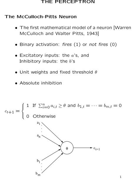
• <strong>The</strong> <strong>first</strong> mathematical model of a neuron [Warren<br />
<strong>McCulloch</strong> and Walter <strong>Pitts</strong>, 1943]<br />
• Binary activation: fires (1) or not fires (0)<br />
• Excitatory inputs: the a’s, and<br />
Inhibitory inputs: the b’s<br />
• Unit weights and fixed threshold θ<br />
• Absolute inhibition<br />
c t+1 =<br />
⎧<br />
⎪⎨<br />
⎪⎩<br />
1 If ∑ n<br />
i=0<br />
a i,t ≥ θ and b 1,t = · · · = b m,t = 0<br />
0 Otherwise<br />
a1<br />
an<br />
.<br />
.<br />
.<br />
θ<br />
c t+1<br />
b1<br />
bm<br />
.<br />
.<br />
.<br />
1
Computing with <strong>McCulloch</strong>-<strong>Pitts</strong> <strong>Neuron</strong>s<br />
a1<br />
2<br />
AND<br />
a2<br />
a1<br />
1 OR<br />
a2<br />
b1<br />
0 NOT<br />
Any task or phenomenon that can be represented as<br />
a logic function can be modelled by a network of<br />
MP-neurons<br />
• {OR, AND, NOT} is functionally complete<br />
• Any Boolean function can be implemented using<br />
OR, AND and NOT<br />
• Canonical forms: CSOP or CPOS forms<br />
• MP-neurons ⇔ Finite State Automata<br />
2
Limitation of MP-neurons and Solution<br />
• Problems with MP-neurons<br />
– Weights and thresholds are analytically determined.<br />
Cannot learn<br />
– Very difficult to minimize size of a network<br />
– What about non-discrete and/or non-binary tasks<br />
• Perceptron solution [Rosenblatt, 1958]<br />
– Weights and thresholds can be determined analytically<br />
or by a learning algorithm<br />
– Continuous, bipolar and multiple-valued versions<br />
– Efficient minimization heuristics exist<br />
x 1<br />
.<br />
.<br />
.<br />
w 1<br />
w n<br />
Σ<br />
y<br />
0<br />
θ<br />
1<br />
f<br />
x n<br />
3
Perceptron<br />
x 0 = 1<br />
x 1<br />
.<br />
.<br />
.<br />
w 1<br />
w n<br />
w 0 = −θ<br />
y<br />
Σ<br />
0<br />
0<br />
1<br />
f<br />
x n<br />
• Architecture<br />
– Input: ⃗x = (x 0 = 1, x 1 , . . . , x n )<br />
– Weight: ⃗w = (w 0 = −θ, w 1 , . . . , w n ), θ = bias<br />
– Net input: y = ⃗w⃗x = ∑ n<br />
i=0<br />
w i x i<br />
– Output f(⃗x) = g( ⃗w⃗x) =<br />
{<br />
0 If ⃗w⃗x < 0<br />
1 If ⃗w⃗x ≥ 0<br />
• Pattern classification<br />
• Supervised learning<br />
• Error-correction learning<br />
4
Perceptron Analysis<br />
• Perceptron’s decision boundary<br />
w 1 x 1 + · · · + w n x n = θ<br />
w 0 x 0 + w 1 x 1 + · · · + w n x n = 0<br />
x2<br />
Separating hyperplane<br />
w<br />
Hyperplane direction<br />
x1<br />
θ<br />
w<br />
• All points<br />
– below the hyperplane have value 0<br />
– on the hyperplane have the same value<br />
– above the hyperplane have value 1<br />
5
Perceptron Analysis<br />
(continued)<br />
• Linear Separability<br />
– A problem (or task or set of examples) is linearly<br />
separable if there exists a hyperplane w 0 x 0 +<br />
w 1 x 1 +· · ·+w n x n = 0 that separates the examples<br />
into two distinct classes<br />
– Perceptron can only learn (compute) tasks that<br />
are linearly separable.<br />
– <strong>The</strong> weight vector ⃗w of the perceptron correspond<br />
to the coefficients of the separating line<br />
• Non-Linear Separability<br />
– Limitations of the perceptron: many real-world<br />
problems are highly non-linear<br />
– Simpe Boolean functions:<br />
∗ XOR, EQUALITY, . . . etc.<br />
∗ Linear, parity, symmetric or . . . functions<br />
6
Perceptron Learning Rule<br />
• Test problem<br />
– Let the set of training examples be<br />
[⃗x 1 = (1, 2), d 1 = 1]<br />
[⃗x 2 = (−1, 2), d 2 = 0]<br />
[⃗x 3 = (0, −1), d 3 = 0]<br />
– <strong>The</strong> bias (or threshold) be b = 0<br />
– <strong>The</strong> initial weight vector be ⃗w = (1, 0.8)<br />
2<br />
1<br />
3<br />
w<br />
We want to obtain a learning algorithm that finds a weight vector<br />
⃗w which will correctly classify (separate) the examples.<br />
7
Perceptron Learning Rule<br />
(continued)<br />
• First input ⃗x 1 is misclassified with positive error. What<br />
to do<br />
• Idea: move hyperplane to separating position<br />
• Solution:<br />
– Move ⃗w closer to ⃗x 1 : add ⃗x 1 to ⃗w.<br />
∗ ⃗w = ⃗w + ⃗x 1<br />
– First rule: positive error rule<br />
If d = 1 and a = 0 then ⃗w new = ⃗w old + ⃗x<br />
2<br />
1<br />
w<br />
3<br />
8
Perceptron Learning Rule<br />
(continued)<br />
• Second input ⃗x 2 is misclassified with negative error<br />
• Solution:<br />
– Move ⃗w away from ⃗x 2 : substract ⃗x 2 from ⃗w.<br />
∗ ⃗w = ⃗w − ⃗x 2<br />
– Second rule: negative error rule<br />
If d = 0 and a = 1 then ⃗w new = ⃗w old − ⃗x<br />
2<br />
1<br />
3<br />
w<br />
9
Perceptron Learning Rule<br />
(continued)<br />
• Third input ⃗x 3 is misclassified with negative error<br />
• Move ⃗w away from to ⃗x 3 : ⃗w = ⃗w − ⃗x 3<br />
2<br />
1<br />
w<br />
3<br />
• <strong>The</strong> perceptron will correctly classify inputs ⃗x 1 , ⃗x 2 , ⃗x 3<br />
if presented to it again. <strong>The</strong>re will be no errors<br />
• Third rule: no error rule<br />
If d = a then ⃗w new = ⃗w old 10
Perceptron Learning Rule<br />
(continued)<br />
• Unified learning rule<br />
⃗w new = ⃗w old + δ⃗x = ⃗w old + (d − a)⃗x<br />
• With learning rate η<br />
⃗w new = ⃗w old + ηδ⃗x = ⃗w old + η(d − a)⃗x<br />
• Choice of learning rate η<br />
– Too large: learning oscillates<br />
– Too small: very slow learning<br />
– 0 < η ≤ 1. Popular choices:<br />
∗ η = 0.5<br />
∗ η = 1<br />
– Variable learning rate η = | ⃗w⃗x|<br />
|⃗x 2 |<br />
– Adaptive learning rate<br />
– . . . etc.<br />
11
Perceptron Learning Algorithm<br />
Initialization: ⃗w 0 = ⃗0;<br />
t = 0;<br />
Repeat<br />
t = t + 1;<br />
Error = 0;<br />
For each training example [⃗x, d ⃗x ] do<br />
net = ⃗w · ⃗x;<br />
a ⃗x = g(net);<br />
δ ⃗x = d ⃗x − a ⃗x ;<br />
Error = Error + |δ ⃗x |;<br />
⃗w t+1 = ⃗w t + η · δ ⃗x · ⃗x;<br />
{<br />
or equivalently,<br />
For 0 ≤ i ≤ n<br />
w i,t+1 = w i,t + η · δ ⃗x · x i ;<br />
}<br />
Until Error = 0;<br />
Save last weight vector;<br />
• Perceptron convergence theorem: [M. Minsky and<br />
S. Papert, 1969] <strong>The</strong> perceptron learning algorithm<br />
terminates if and only if the task is linearly separable<br />
• Cannot learn non-linearly separable functions<br />
12
Perceptron Learning Algorithm<br />
(continued)<br />
• Termination criteria<br />
– Assured for small enough η and l.s. functions<br />
– For non-l.s. functions: halt when number of misclassifications<br />
is minimal<br />
• Problem representation<br />
– Non-numeric inputs: encode into numeric form<br />
– Multiple-class problem:<br />
∗ Use single-layer network<br />
∗ Each output node corresponds to one class<br />
∗ A u-neuron network can classify inputs into 2 u<br />
classes<br />
• Variations of perceptron<br />
– Bipolar vs. binary encodings<br />
– Threshold vs. signum functions<br />
13
Pocket Algorithm<br />
• Robust classification for linearly non-separable problems<br />
• Find ⃗w such that such that the number of misclassifications<br />
is as small as possible.<br />
Initialization: ⃗w 0 = PerceptronLearning;<br />
Error ⃗w0 = number of misclassifications of ⃗w 0 ;<br />
Pocket = ⃗w 0 ;<br />
t = 0;<br />
Repeat<br />
t = t + 1;<br />
⃗w t = PerceptronLearning;<br />
If Error ⃗wt < Error ⃗wt−1 <strong>The</strong>n<br />
Pocket = ⃗w t ;<br />
Until t = MaxIterations;<br />
Best weight so far is stored in Pocket;<br />
• Initial weight in PerceptronLearning should be random<br />
• Presentation of training examples in<br />
PerceptronLearning should be random<br />
• Slow but robust learning for non-separable tasks<br />
14
Adaline<br />
x 0 = 1<br />
x 1<br />
.<br />
.<br />
.<br />
w 1<br />
w n<br />
Σ<br />
w 0<br />
y<br />
f<br />
x n<br />
• Architecture<br />
– Input: ⃗x = (x 0 = 1, x 1 , . . . , x n )<br />
– Weight: ⃗w = (w 0 = −θ, w 1 , . . . , w n ), θ = bias<br />
– Net input: y = ⃗w⃗x = ∑ n<br />
i=0<br />
w i x i<br />
– Output f(⃗x) = g( ⃗w⃗x) = ⃗w⃗x<br />
• Pattern classification<br />
• Supervised learning<br />
• Error-correction learning<br />
15
Adaline Analysis<br />
• Adaline’s decision boundary<br />
w 0 x 0 + w 1 x 1 + · · · + w n x n = 0<br />
x2<br />
Separating hyperplane<br />
w<br />
θ<br />
w 1<br />
Hyperplane direction<br />
θ x1<br />
w2<br />
θ<br />
w<br />
• <strong>The</strong> Adaline<br />
– has a decision boundary like the perceptron<br />
– can be used to classify objects into two categories<br />
– has same limitation as the perceptron<br />
16
Adaline Learning Principle<br />
• Data fitting (or linear regression)<br />
– Set of measurements: {(x, d x )}<br />
– Find w and b such that<br />
d x ≈ wx + b<br />
or more specifically,<br />
d i = wx i + b + ε i = y i + ε i<br />
where<br />
∗ ε i = instantaneous error<br />
∗ y i = linearly fitted value<br />
∗ w = line slope, b = d-axis intercept (or bias)<br />
d<br />
3.5 x<br />
3<br />
2.5<br />
2<br />
1.5<br />
1<br />
0.5<br />
0 2 4 6 8<br />
x<br />
10 12<br />
17
Adaline Learning Principle<br />
(continued)<br />
• Best fit problem: find the best choice of ( ⃗w, b) such<br />
that the fitted line passes closest to all points<br />
• Solution: Least squares<br />
– Minimize sum of squared errors (SSE) or mean of<br />
squared errors (MSE)<br />
– Error ε ⃗x = d ⃗x − ˜d ⃗x where ˜d ⃗x = ⃗w⃗x + b<br />
– MSE:<br />
N∑<br />
J = 1 N<br />
ε⃗x 2 i<br />
i=1<br />
d<br />
3.5 x<br />
3<br />
2.5<br />
2<br />
1.5<br />
1<br />
0.5<br />
0 2 4 6 8<br />
x<br />
10 12<br />
18
Adaline Learning Principle<br />
(continued)<br />
• <strong>The</strong> minimum MSE, called the least mean square<br />
(LMS) can be obtained analytically:<br />
and solve for ⃗w and b<br />
δJ<br />
δ ⃗w = 0<br />
δJ<br />
δb = 0<br />
• Pattern classification can be interpreted as a linear<br />
• LMS is difficult to obtain for larger dimensions (complex<br />
formula) and larger data sets<br />
• Adaline:<br />
– Learns by minimizing the MSE<br />
– Not sensitive to noise<br />
– Powerful and robust learning<br />
19
Adaline Learning Algorithm<br />
• Gradient descent<br />
– A learning example: [⃗x, d ⃗x ]<br />
– Actual output: net ⃗x =<br />
– Desired output: d ⃗x<br />
– Squared error: E ⃗x = (d ⃗x − net ⃗x ) 2<br />
– Gradient of E ⃗x :<br />
∇E ⃗x = δE ⃗x<br />
δ ⃗w = (δE ⃗x<br />
δw 0<br />
, δE ⃗x<br />
δw 1<br />
, . . . , δE ⃗x<br />
δw n<br />
)<br />
– E ⃗x is minimal if and only if ∇E ⃗x = 0<br />
– Negative gradient of E ⃗x :<br />
−∇E ⃗x<br />
gives direction of steepest descent to the minimum<br />
– Gradient descent:<br />
∆ ⃗w = −η∇E ⃗x = − δE ⃗x<br />
δ ⃗w<br />
20
Adaline Learning Algorithm<br />
(continued)<br />
• Widrow-Hoff delta rule<br />
–<br />
δE ⃗x<br />
δw i<br />
= 2(d ⃗x − net ⃗x ) δ(−net ⃗x )<br />
δ ⃗w i<br />
= (d ⃗x − net ⃗x ) δ(− ∑ n<br />
j=0<br />
w j x j )<br />
δ ⃗w i<br />
= −(d ⃗x − net ⃗x )x i<br />
• ⇒ Learning rule:<br />
⃗w new = ⃗w old + η(d ⃗x − net ⃗x )⃗x<br />
21
Adaline Learning Algorithm<br />
(continued)<br />
Initialization: ⃗w 0 = ⃗0;<br />
t = 0;<br />
Repeat<br />
t = t + 1;<br />
For each training example [⃗x, d ⃗x ] do<br />
net ⃗x = ⃗w · ⃗x;<br />
a ⃗x = g(net ⃗x ) = net ⃗x ;<br />
δ ⃗x = d ⃗x − a ⃗x ;<br />
⃗w t+1 = ⃗w t + η · δ ⃗x · ⃗x;<br />
{<br />
or equivalently,<br />
For 0 ≤ i ≤ n<br />
w i,t+1 = w i,t + η · δ ⃗x · x i ;<br />
}<br />
Until MSE (⃗w) is minimal;<br />
Save last weight vector;<br />
• Can be used for function approximation task as well<br />
22