3d representation of liposomes using dupin cyclides - SEE
3d representation of liposomes using dupin cyclides - SEE
3d representation of liposomes using dupin cyclides - SEE

Create successful ePaper yourself
Turn your PDF publications into a flip-book with our unique Google optimized e-Paper software.
3D REPRESENTATION OF LIPOSOMES<br />
USING DUPIN CYCLIDES<br />
Lionel Garnier, Sebti Foufou<br />
LE2i, UMR CNRS 5158, University <strong>of</strong> Burgundy, B.P. 47870, 21 078 Dijon Cedex, France<br />
@u-bourgogne.fr<br />
ABSTRACT<br />
Liposomes are vesicles used in several domains:<br />
medicine, biology and biochemistry. The aim <strong>of</strong> this paper<br />
is to show how Dupin <strong>cyclides</strong> (Algerbraci surfaces<br />
<strong>of</strong> degree 4) can be used to get a 3D <strong>representation</strong> <strong>of</strong> <strong>liposomes</strong>,<br />
which allows easy visualization and may facilitates<br />
the simulation <strong>of</strong> the various manipulation one can<br />
need to do with <strong>liposomes</strong>.<br />
Dupin <strong>cyclides</strong> was introduced time in 1822 by the<br />
French mathematician Pierre-Charles Dupin. Although,<br />
they have a number <strong>of</strong> interesting geometric properties<br />
that make them suitable for geometric modeling and 3D<br />
<strong>representation</strong>, their use in the nowadays modeling tools<br />
is not yet considered. The conversion <strong>of</strong> Dupin <strong>cyclides</strong><br />
into commonly used 3 D <strong>representation</strong> surfaces, such as<br />
rational biquadratic Bézier parametric surfaces, is therefore<br />
necessary and it also is discussed in this paper. We<br />
show examples <strong>of</strong> entire or part <strong>of</strong> liposome represented<br />
as Dupin <strong>cyclides</strong> together with their Bèzier conversion.<br />
KEY WORDS<br />
Liposome, Dupin <strong>cyclides</strong>, torus <strong>of</strong> Willmore, Rational<br />
Biquadratic Bézier Patches, 3D <strong>representation</strong>.<br />
1 Introduction<br />
Since A. Bangham discovered <strong>liposomes</strong> about 30 years<br />
ago, these have been used in several domains as biology,<br />
biochemistry and medicine [14]. They can play the role<br />
<strong>of</strong> drug carriers and can be charged <strong>of</strong> a large variety <strong>of</strong><br />
molecules: small drug molecules, proteins, nucleotides<br />
and plasmids. This method permits to introduce a gene<br />
<strong>of</strong> interest in a cell. Indeed, Dr. Xiaoyang Qi at the<br />
Cincinnati children’s research foundation has developed a<br />
unique composition for modulation <strong>of</strong> highly active growing<br />
cell. The complex is formed by a fusogenic protein or<br />
peptide derived from prosaposin associated with a liposome<br />
which may also contain a drug material in a pharmaceutically<br />
acceptable carrier to improve the delivery <strong>of</strong><br />
that material across the biological membrane.<br />
In 1990, U. Seifert [18] prooved that, besides the<br />
spheres and surfaces which are characterized only by continuous<br />
deformations, there are blisters <strong>of</strong> toric kind: the<br />
torus <strong>of</strong> Willmore (the ratio <strong>of</strong> the major radius to the<br />
minor radius is √ 2) and the images <strong>of</strong> this torus by an<br />
inversion i.e. <strong>cyclides</strong> <strong>of</strong> Dupin. Topological genus <strong>of</strong><br />
these two surfaces is 1, since it is necessary to add a handle<br />
to the sphere to obtain a surface equivalent to the one<br />
<strong>of</strong> these two surfaces [13]. In 1965, Willmore conjectured<br />
that directional surfaces <strong>of</strong> kind 1 having an axis<br />
<strong>of</strong> symmetry whose energy <strong>of</strong> curvature is weakest, are<br />
the torus <strong>of</strong> Willmore [21] and its images by inversion.<br />
This result was checked in experiments. The 3D <strong>representation</strong><br />
<strong>of</strong> <strong>liposomes</strong> needs the use <strong>of</strong> two primitives:<br />
spheres and Dupin <strong>cyclides</strong> (a torus is a particular Dupin<br />
cyclide). Moreover, some particular Dupin <strong>cyclides</strong> are<br />
double spheres. So, Dupin <strong>cyclides</strong> seem to be sufficient<br />
to represent all the possible forms <strong>of</strong> <strong>liposomes</strong>.<br />
Except the quadrics [4] and the tori <strong>of</strong> revolution [4],<br />
surfaces available in the modelers are parametric surfaces<br />
such as NURBS, B-Splines and Bézier [5, 15, 9], but<br />
Dupin <strong>cyclides</strong> are not proposed. Dupin <strong>cyclides</strong> are algebraic<br />
surfaces introduced for the first time in 1822 by<br />
the French mathematician Pierre-Charles Dupin [8]. They<br />
have a low algebraic degree: at most 4. Liposomes can<br />
be modelled by quartic Dupin <strong>cyclides</strong>. These Dupin cy-
£<br />
£¢<br />
¢<br />
¡<br />
¡<br />
¥¤<br />
¤<br />
clides have a parametric equation and two equivalent implicit<br />
equations [10, 7] and they have been studied by a<br />
several mathematicians [6, 7, 4]. Recently, a number <strong>of</strong><br />
authors used them in Computer Aided Geometric Design,<br />
examples <strong>of</strong> such works are: Their use for the blending<br />
<strong>of</strong> quadrics [16, 17, 2, 3]; Their <strong>representation</strong> as Rational<br />
Biquadratic Bézier Patches (RBBPs) [16, 20, 1, 12];<br />
Their NURBS conversion [22].<br />
This paper is organized as follows: section 2 presents<br />
the needed mathematical background (RBBP, torus <strong>of</strong><br />
Willmore, inversion, Dupin <strong>cyclides</strong>). Section 3 presents<br />
the conversion <strong>of</strong> Dupin <strong>cyclides</strong> into RBBPs <strong>using</strong> an algorithm<br />
proposed by Pratt [16]. Section 4 presents two<br />
new conversion algorithms. Section 5 presents the conclusion.<br />
2 Background<br />
2.1 Rational Biquadratic Bézier Patches<br />
(RBBP)<br />
The three Bernstein polynomial <strong>of</strong> degree 2 are:<br />
B i (t) = C i 2 t i (1 − t) 2−i (1)<br />
where i ∈ [[0; 2]]. A point M (u, v), (u, v) ∈ [0; 1] 2 on a<br />
RBBP is given by:<br />
Ω<br />
z<br />
∆<br />
R<br />
¥ O<br />
r<br />
C<br />
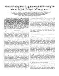
Figure 1: A torus <strong>of</strong> revolution.<br />
So, in P, ∆ and ∆ ′ are the axis <strong>of</strong> the reference system.<br />
Let R = ΩO, the equation <strong>of</strong> C is y (θ) = (R + r cos θ)<br />
and z (θ) = r sin θ and the parametric equation <strong>of</strong> the<br />
torus is:<br />
⎛<br />
Γ T (θ, ψ) = ⎝<br />
y<br />
(R + r cos θ) cos ψ<br />
(R + r cos θ) sin ψ<br />
r sin θ<br />
⎞<br />
⎠ (3)<br />
where θ ∈ [0; 2π], ψ ∈ [0; 2π]. If R = r √ 2, the torus is<br />
called Willmore torus.<br />
2.3 Inversion<br />
Let E be the affine space, Ω a point belonging to E, k<br />
a number not equal to 0. An inversion is an application<br />
i : E −{Ω} −→ E −{Ω} [16] defined by: ∀M ∈ E −{Ω},<br />
M ′ = i (M) ⇐⇒<br />
−−→<br />
ΩM ′ · −−→ ΩM = k<br />
i.e.<br />
−−→<br />
ΩM ′ =<br />
k<br />
ΩM 2 · −−→ ΩM (4)<br />
−−−−−−→<br />
OM (u, v) =<br />
2∑<br />
2∑<br />
i=0 j=0<br />
2∑<br />
i=0 j=0<br />
B ij (u, v) −−→ OP ij<br />
2∑<br />
B ij (u, v)<br />
(2)<br />
2.4 Quartic Dupin <strong>cyclides</strong><br />
where (P ij ) 0≤i,j≤2<br />
are control points, (w ij ) 0≤i,j≤2<br />
are<br />
weights and B ij (u, v) = w ij B i (u) B j (v) [16].<br />
2.2 Torus <strong>of</strong> Willmore<br />
Let O be the center and r the radius <strong>of</strong> a circle C in a plane<br />
P. Let ∆ be a straight line such as O does not belong<br />
to ∆. The torus <strong>of</strong> revolution, figure 1, is produced by<br />
rotating the circle C, called meridian [4], about the axis<br />
∆. In the plane P, let Ω be the intersection between ∆<br />
and ∆ ′ , its perpendicular straight line passing through O.<br />
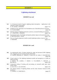
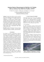
Figure 2: Three kinds <strong>of</strong> Dupin <strong>cyclides</strong>. Left: ring, 0 ≤<br />
|c| ≤ |µ| ≤ |a|. Middle: horned, 0 < |µ| ≤ |c| < |a|.<br />
Right: half spindle, 0 ≤ |c| ≤ |a| < |µ|.<br />
It is possible to define Dupin <strong>cyclides</strong> in various equivalent<br />
ways: Liouville showed that a Dupin cyclide is the<br />
image <strong>of</strong> a cone <strong>of</strong> revolution or a torus <strong>of</strong> revolution or<br />
a cylinder <strong>of</strong> revolution under an inversion; A Dupin cyclide<br />
is the envelope <strong>of</strong> spheres centered on a given conic<br />
and orthogonal to a given fixed sphere, called sphere <strong>of</strong><br />
2
inversion: the latter is centered on the focal axis <strong>of</strong> the<br />
Dupin cyclide [6, 7]; A Dupin cyclide is the envelope surface<br />
<strong>of</strong> a set <strong>of</strong> spheres, the centers M <strong>of</strong> which lies on a<br />
given conic with focus F , and the radius <strong>of</strong> which is such<br />
that the distance F M + R is a given constant (this definition<br />
is due to Maxwell); A Dupin cyclide is the envelope<br />
surface <strong>of</strong> the spheres tangent to three given fixed spheres<br />
[8].<br />
equation:<br />
⎛<br />
Γ d (θ, ψ) =<br />
⎜<br />
⎝<br />
µ (c − a cos θ cos ψ) + b 2 cos θ<br />
a − c cos θ cos ψ<br />
b sin θ × (a − µ cos ψ)<br />
a − c cos θ cos ψ<br />
b sin ψ × (c cos θ − µ)<br />
a − c cos θ cos ψ<br />
⎞<br />
⎟<br />
⎠<br />
(5)<br />
where θ ∈ [0; 2π], ψ ∈ [0; 2π].<br />
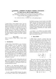
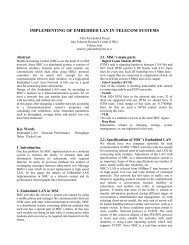
Figure 3: Left: Three medical images <strong>of</strong> Liposomes.<br />
Right: Liposomes modelled with Willmore torus and<br />
Dupin cyclide<br />
Quartic Dupin <strong>cyclides</strong> depend on three independent<br />
parameters a, c and µ with |c| ≤ |a|. It is convenient to<br />
define b = √ a 2 − c 2 . According to the parameter values,<br />
there are three kinds <strong>of</strong> Dupin <strong>cyclides</strong>: ring, horned and<br />
spindle, figure 2. The ε-<strong>of</strong>fset <strong>of</strong> a Dupin cyclide which<br />
parameters a, c and µ is a Dupin cyclide which parameters<br />
a, c and µ + ε [19].<br />
Except the torus <strong>of</strong> Willmore, the other adjustable surfaces<br />
with a topological genus equal to 1, having a weakest<br />
energy <strong>of</strong> curvature, are the images <strong>of</strong> Willemore torus<br />
under an inversion i.e. they are particular Dupin <strong>cyclides</strong>,<br />
figure 3. This result was checked in experiments in the<br />
forms taken by <strong>liposomes</strong>, figure 3 (left). Figure 3 (right)<br />
shows 3D <strong>representation</strong>s <strong>of</strong> two two <strong>liposomes</strong> <strong>using</strong> a<br />
Willmore torus and a Dupin cyclide. The radii <strong>of</strong> the torus<br />
are R = 4 √ 2 and r = 4. The Dupin cyclide is the image<br />
<strong>of</strong> this torus under an inversion, the coordinates <strong>of</strong> the<br />
center are (1; 0; 0) and the rapport is k = 8. Dupin parameters<br />
are: a = 480√ 2<br />
161<br />
≃ 4, 22, µ = 544<br />
161<br />
≃ 3, 38 and<br />
c = 256√ 2<br />
161<br />
≃ 2, 25. The values <strong>of</strong> parameters a, c and<br />
µ are computed <strong>using</strong> two principal circles <strong>of</strong> the Dupin<br />
cyclide [16, 11].<br />
Two equivalent implicit equations <strong>of</strong> a Dupin cyclide were<br />
obtained by Darboux early in the last century by computing<br />
the implicit equation <strong>of</strong> the envelope <strong>of</strong> the spheres<br />
defining the Dupin cyclide [7]. The same results are also<br />
given by Forsyth [10]. A Dupin cyclide has a parametric<br />
3 Conversion <strong>of</strong> Dupin <strong>cyclides</strong> into RBBP<br />
In this section, the parameters a, c and µ <strong>of</strong> the Dupin<br />
cyclide and the bounds θ 0 , θ 0 , ψ 0 and ψ 1 <strong>of</strong> the part <strong>of</strong><br />
the Dupin cyclide to convert are given.<br />
Curves plotted on a RBBP with one variable u or v constant<br />
are conics. The lines <strong>of</strong> curvature <strong>of</strong> Dupin <strong>cyclides</strong><br />
are particular conics: circles. So, it is possible to convert a<br />
part (region) <strong>of</strong> a Dupin cyclide into a RBBP. This part is<br />
defined by four lines <strong>of</strong> curvature: γ θ0 : ψ ↦→ Γ d (θ 0 , ψ),<br />
γ θ1 : ψ ↦→ Γ d (θ 1 , ψ), γ ψ0 : θ ↦→ Γ d (θ, ψ 0 ) , γ ψ1 : θ ↦→<br />
Γ d (θ, ψ 1 ). To this end, we have to compute nine control<br />
points (P ij ) 0≤i,j≤2<br />
and the nine weights (w ij ) 0≤i,j≤2<br />
.<br />
Several conversion algorithms have been presented:<br />
K. Ueda uses matrix and resolve systems <strong>of</strong> linear<br />
equations [20]. G. Albrecht converts a piece <strong>of</strong> a cone<br />
<strong>of</strong> revolution into RBBP. The image <strong>of</strong> this RBBP is an<br />
RBBP representing a piece <strong>of</strong> symmetric horned Dupin<br />
cyclide (µ = 0 and c ≠ 0). The kind <strong>of</strong> the Dupin<br />
cyclide can be modified by taking a ε-<strong>of</strong>fset <strong>of</strong> Dupin<br />
cyclide [1]. Some examples <strong>of</strong> results can be found on<br />
site: http://www.univ-valenciennes.fr/<br />
macs/caomacs/<strong>dupin</strong>.htm. We have developed<br />
an algorithm that uses barycentric properties <strong>of</strong> Dupin<br />
<strong>cyclides</strong> and the Bézier <strong>representation</strong>s <strong>of</strong> circular arcs<br />
[12]. In this paper, we consider in more details the<br />
conversion algorithm presented by M. Pratt in [16]. We<br />
show and discuss some results <strong>of</strong> this algorithm with<br />
possible improvements.<br />
In this algorithm, the coordinates <strong>of</strong> control points and<br />
weights are calculated directly from the parametric equation<br />
<strong>of</strong> the Dupin cyclide, equation (5), and from the<br />
3
ounds θ 0 , θ 0 , ψ 0 and ψ 1 . In fact, M. Pratt writes circular<br />
functions as rational fractions (cos θ = 1−t2<br />
1+t<br />
and 2<br />
sin θ =<br />
2t<br />
1+t<br />
) in <strong>using</strong> trigonometric relations:<br />
2<br />
cos (θ) = 1 − ( )<br />
tan2 θ<br />
2<br />
1 + tan ( ), sin (θ) = 2 tan ( )<br />
θ<br />
2<br />
2 θ<br />
1 + tan ( ) (6)<br />
2 θ<br />
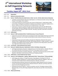
Figure 4: Wrong conversion <strong>of</strong> a piece <strong>of</strong> liposome into<br />
RBBP, |θ 0 − θ 1 | > π. Left: Dupin cyclide. Right: Dupin<br />
2<br />
2<br />
cyclide and RBBP.<br />
where θ ∈ R − πZ. To determine the nine control points<br />
(P ij ) 0≤i,j≤2<br />
and the nine weights (w ij ) 0≤i,j≤2<br />
, he defines<br />
the numbers: ţ ű θ0<br />
g 0 = tan<br />
g 1 = g ţ ű computed as if θ 0 = − 2π 3<br />
and θ 1 = 0, which does not<br />
0 + g 2<br />
θ1<br />
g 2 = tan<br />
allow to obtain the right conversion. So, the conditions<br />
ţ 2 ű<br />
ţ2<br />
ű<br />
2<br />
ψ0<br />
ψ1<br />
h 0 = tan h 2 = tan<br />
h 1 = h 0 + h 2<br />
are:<br />
ţ2<br />
ű<br />
2<br />
2<br />
|θ<br />
ţ ű<br />
0 − θ 1 | < π and |ψ 0 − ψ 1 | < π (11)<br />
(7)<br />
G 0 = tan 2 θ0<br />
G 1 = g 0 × g 1 G 2 = tan 2 θ1<br />
ţ 2 ű<br />
ţ 2 The non-observance <strong>of</strong> the constraint |θ<br />
ű<br />
0 − θ 1 | < π is<br />
H 0 = tan 2 ψ0<br />
H 1 = h 0 × h 1 H 2 = tan 2 ψ1 showed by figure 4. On the left picture, one can see the<br />
2<br />
2 patch <strong>of</strong> Dupin cyclide. On the right picture, one can<br />
Immediately, we note that π is a forbidden value. For see the Dupin cyclide patch and its wrong corresponding<br />
RBBP. In fact, the RBBP is the complementary <strong>of</strong><br />
(i; j) ∈ [[0, 2]] 2 1<br />
, let be P ij = ̂Pij where:<br />
a−c 1−G i<br />
1+G × 1−H j<br />
i 1+H j the Dupin cyclide patch (for the values θ). However, it<br />
0<br />
b 2 1 − G i<br />
− µa 1 − G i<br />
× 1 − H 1<br />
j<br />
+ µc is now possible to take values θ 0 , θ 1 , ψ 0 and ψ 1 such<br />
1 + G i 1 + G i 1 + H j as π ∈ ]θ ţ<br />
g i<br />
2b a − µ 1 − H ű<br />
0 ; θ 1 [ and/or π ∈ ]ψ 0 ; ψ 1 [. Indeed, a piece<br />
j<br />
<strong>of</strong> liposome, figure 3, is converted into RBBP, figure 5.<br />
cP ij =<br />
1 + G i 1 + H j (8) The bounds <strong>of</strong> the piece are: θ 0 = 0, θ 1 = π 3 , ψ 0 = π 2<br />
ţ<br />
B<br />
@ 2b c 1 − G ű<br />
i hj<br />
and ψ 1 = 4π<br />
C<br />
3<br />
. Left picture shows the Dupin cyclide and<br />
− µ<br />
A the piece to convert. Pratt’s algorithm produces a wrong<br />
1 + G i 1 + H j<br />
RBBP, middle picture, whereas the new algorithm gives a<br />
and the weight w ij is given by:<br />
correct conversion, right picture. So, it is now possible to<br />
convert some new <strong>liposomes</strong> pieces.<br />
w ij = a (1 + G i ) (1 + H j ) − c (1 − G i ) (1 − H j ) (9)<br />
The trigonometric values <strong>of</strong> angles θ 0 , θ 1 , ψ 0 and ψ 1 are<br />
used to determine the elements <strong>of</strong> the equation (7), which<br />
are thereafter introduced into the formula (8) to obtain<br />
the coordinates <strong>of</strong> control points, and into formula (9)<br />
to obtain weights. In case one θ 0 = 2π 3 and θ 1 = 4π 3 , Figure 5: Conversions <strong>of</strong> a piece <strong>of</strong> liposome into RBBP.<br />
the discontinuity <strong>of</strong> the function x ↦→ tan ( )<br />
x<br />
Left: Dupin cyclide. Middle: conversion <strong>using</strong> Pratt’s<br />
2 in π<br />
algorithm. Right: conversion <strong>using</strong> a variant <strong>of</strong> Pratt’s<br />
modulo 2π makes that weights and control points will be<br />
calculated as if θ 0 = − 2π 3<br />
and θ 1 = 2π algorithm.<br />
3<br />
, which makes it<br />
impossible to obtain the correct conversion [12].<br />
One way to deal with the above mentioned drawback<br />
is to take the absolute value in the weights<br />
computation formula as follows (for (i, j) ∈ [[0; 2]]):<br />
w ij = |a (1 + G i ) (1 + H j ) − c (1 − G i ) (1 − H j )| (10)<br />
Moreover, if θ 0 = 0 and θ 1 = 4 π 3 , control points are<br />
For each variable θ and ψ, conditions <strong>of</strong> formula (11)<br />
imply that at least three values are necessary. So, to represent<br />
a complete Dupin cyclide, at least nine RBBPs are<br />
necessary. Figure 6 shows two examples <strong>of</strong> conversion.<br />
Of course, the problem with π remains. So, it is not<br />
possible to use this algorithm to convert some Dupin <strong>cyclides</strong><br />
carrying out a blending between a plane and a cylinder<br />
<strong>of</strong> revolution. For this reason, we have to present the<br />
4
Figure 6: A liposome converted into RBBPs. Left: Dupin<br />
cyclide. Middle: sixteen RBBPs. Right: nine RBBPs.<br />
following algorithm.<br />
4 Re-parametrisation and affine transformation<br />
Until now, the parameters a, c and µ <strong>of</strong> Dupin <strong>cyclides</strong><br />
have always been positive. In this section, parameters µ<br />
and c can be negative. Theorem 1 gives the affine transformation<br />
to apply when we modify the sign <strong>of</strong> c and/or µ.<br />
The conversion algorithm proposed here is based on the<br />
Pratt’s algorithm discussed in the previous section. Using<br />
the new method, the conversion can be done in three steps:<br />
re-parametrization <strong>of</strong> the Dupin cyclide; use for Pratt’s algorithm;<br />
choice <strong>of</strong> the appropriate affine transformation.<br />
Theorem 1 :<br />
Let S be a Dupin cyclide with positive parameters a, c<br />
and µ. Let S c (resp S µ ) be the Dupin cyclide obtained by<br />
replacing c with −c (resp. µ with −µ). In the same way,<br />
S c,µ is the Dupin cyclide with parameters a, −c and −µ.<br />
Let ˜θ + (Γ d ) (resp. ˜ψ + (Γ d )) be the surface obtained by<br />
the re-parametrization θ ↦−→ θ + π (resp. ψ ↦−→ ψ + π).<br />
Let ˜θ − (Γ d ) (resp. ˜ψ − (Γ d )) be the surface obtained by<br />
the re-parametrization θ ↦−→ π − θ (resp. ψ ↦−→ π − ψ).<br />
Let r z (resp. r y ) be the rotation by π around the<br />
axis<br />
(O, −→ )<br />
k 0 (resp. (O, −→ j 0 )). Let s y (resp. s x ) be<br />
(O, −→ ı 0 , −→ )<br />
k 0<br />
the reflexion compared with the plane<br />
(O, −→ j 0 , −→ )<br />
k 0 ). Then:<br />
)<br />
1. S = r z<br />
(˜θ+ (S c )<br />
)<br />
and S = s x<br />
(˜θ− (S c ) .<br />
))<br />
(resp.<br />
(<br />
2. S = s x ˜ψ+<br />
(˜θ− (S µ ) and S =<br />
( ))<br />
r y ˜ψ−<br />
(˜θ− (S µ ) .<br />
3. S = ˜ψ<br />
( )<br />
+ (S c,µ ) and S = s z ˜ψ− (S c,µ ) .<br />
Figure 7: Conversion <strong>of</strong> a part <strong>of</strong> liposome into RBBP<br />
by applying item 1 <strong>of</strong> theorem 1. Left: Dupin cyclide<br />
representing the part. Right: the computed RBBP.<br />
Two conversions <strong>of</strong> a part <strong>of</strong> liposome (figure 3), into<br />
RBBP, which were impossible until now, are shown on<br />
figures 7 through 9. First, figure 7, the Pratt’s algorithm<br />
is applied <strong>using</strong> item 1. The bounds <strong>of</strong> the liposome piece<br />
are: θ 0 = 3π 4 , θ 1 = π, ψ 0 = −2π<br />
3<br />
and ψ 1 = − π 4 .<br />
Figure 8: Conversion <strong>of</strong> a part <strong>of</strong> liposome into RBBP by<br />
applying item 3 <strong>of</strong> theorem 1. Left: Dupin cyclide. Right:<br />
RBBP.<br />
Second, figure 8, the Pratt’s algorithm is applied <strong>using</strong><br />
item 3. The bounds <strong>of</strong> the part <strong>of</strong> liposome are θ 0 = − π 4 ,<br />
θ 1 = 0, ψ 0 = −π and ψ 1 = − π 4 .<br />
Figure 9: Conversion <strong>of</strong> a liposome into fours RBBPs.<br />
Left: Dupin cyclide. Right: RBBPs.<br />
Moreover, it is possible to convert a complete liposome<br />
<strong>using</strong> a combination <strong>of</strong> algorithms, figure 9. The bounds<br />
<strong>of</strong> the part <strong>of</strong> liposome are θ 0 = 3π 4 , θ 1 = 7π 6 , ψ 0 = 3π 4<br />
and ψ 1 = 5π 4 . S 1 is obtained by <strong>using</strong> Pratt’s algorithm.<br />
S 2 (resp. S 3 , S 4 ) is obtained by <strong>using</strong> the second improvement,<br />
item 2 (resp. item 3, item 1).<br />
5
5 Conclusion<br />
To make 3D <strong>representation</strong>s <strong>of</strong> <strong>liposomes</strong> with classical<br />
modelers, we have studied the use <strong>of</strong> Dupin <strong>cyclides</strong>,<br />
some examples <strong>of</strong> theses <strong>representation</strong>s are shown. The<br />
conversion <strong>of</strong> Dupin <strong>cyclides</strong> into RBBPs simplifies the<br />
use <strong>of</strong> the proposed <strong>representation</strong>s in common geometric<br />
modeling tools, we have discussed two conversion algorithms<br />
and given two illustrating conversion results.<br />
References<br />
[1] G. Albrecht and W. Degen. Construction <strong>of</strong> Bézier<br />
rectangles and triangles on the symetric Dupin horn<br />
cyclide by means <strong>of</strong> inversion. Computer Aided Geometric<br />
Design, 14(4):349–375, 1996.<br />
[2] S. Allen and D. Dutta. Cyclides in pure blending<br />
I. Computer Aided Geometric Design, 14(1):51–75,<br />
1997. ISSN 0167-8396.<br />
[3] S. Allen and D. Dutta. Cyclides in pure blending II.<br />
Computer Aided Geometric Design, 14(1):77–102,<br />
1997. ISSN 0167-8396.<br />
[4] M. Berger. Géométrie II, volume 2. Springer-Verlag,<br />
2rd edition, 1987.<br />
[5] P. Bézier. Courbe et surface, volume 4. Hermès,<br />
Paris, 2ème edition, Octobre 1986.<br />
[6] G. Darboux. Sur une Classe Remarquable de<br />
Courbes et de Surfaces Algébriques et sur la Théorie<br />
des Imaginaires. Gauthier-Villars, 1873.<br />
[7] G. Darboux. Principes de géométrie analytique.<br />
Gauthier-Villars, 1917.<br />
[8] C. P. Dupin. Application de Géométrie et de<br />
Méchanique la Marine, aux Ponts et Chaussées, etc.<br />
Bachelier, Paris, 1822.<br />
[9] J. Foley, A. Van Dam, D. Freiner, and J. Hughes.<br />
Computer Graphics : Principles and Practice. Addison<br />
Wesley, 2 edition, 1990.<br />
[10] A. R. Forsyth. Lecture on Differential Geometry <strong>of</strong><br />
Curves and Surfaces. Cambridge University Press,<br />
1912.<br />
[11] S. Foufou and L. Garnier. Dupin cyclide blends between<br />
quadric surfaces for shape modeling. In EU-<br />
ROGRAPHICS 2004, 30 august - 3 september 2004.<br />
[12] L. Garnier, S. Foufou, and M. Neveu. Conversion de<br />
<strong>cyclides</strong> de Dupin en carreaux de Bézier rationnels<br />
biquadriques. In Actes des 15 emes journées AFIG,<br />
pages 231–240, Lyon, France, December 2002.<br />
[13] F. Jlicher. The Morphology <strong>of</strong> Vesicles <strong>of</strong> Higher<br />
Topological Genus: Conformal Degeneracy and<br />
Conformal Modes. J. Phys. II France, 6, 1996.<br />
[14] Naoaki Ono and Takashi Ikegami. Model <strong>of</strong> selfreplicating<br />
cell capable <strong>of</strong> self-maintenance. In European<br />
Conference on Artificial Life, pages 399–<br />
406, 1999.<br />
[15] L. Piegl and W. Tiller. The NURBS Book. Springer,<br />
2nd edition, 1997.<br />
[16] M. J. Pratt. Cyclides in computer aided geometric<br />
design. Computer Aided Geometric Design, 7(1-<br />
4):221–242, 1990.<br />
[17] M. J. Pratt. Cyclides in computer aided geometric<br />
design II. Computer Aided Geometric Design,<br />
12(2):131–152, 1995.<br />
[18] U. Seifert. Vesicules <strong>of</strong> toroidal topology. Phys. Rev.<br />
Lett., 66(18):2404–2407, 1991.<br />
[19] C. K. Shene. Do blending and <strong>of</strong>fsetting commute<br />
for Dupin <strong>cyclides</strong>. Computer Aided Geometric Design,<br />
17(9):891–910, 2000.<br />
[20] K. Ueda. Normalized Cyclide Bézier Patches. In<br />
M. Daehlen, T. Lyche, and L.L. Schumaker, editors,<br />
Mathematical Methods for Curves and Surfaces,<br />
pages 507–516, Nashville, USA, 1995. Vanderbilt<br />
University Press. Proc. <strong>of</strong> the International Conference<br />
on Math. Methods in CAGD, Ulvik, Norway,<br />
June 16-21, 1994.<br />
[21] T.J. Willmore. Note on embedded surfaces. Analele<br />
Stiinfice ale Universitatii Al. I. Cuza, 11:493–496,<br />
1965.<br />
[22] X. Zhou and W. Strasser. A NURBS aproach to<br />
<strong>cyclides</strong>. Computers In Industry, 19(2):165–174,<br />
1992.<br />
6