The Steepest Descent Algorithm for Unconstrained Optimization and ...

The Steepest Descent Algorithm for Unconstrained
Optimization
and a
Bisection Line-search Method
Robert M. Freund
February, 2004
2004 Massachusetts Institute of Technology.
1

1 The Algorithm
The problem we are interested in solving is:
P : minimize f(x)
s.t. x ∈R n ,
where f(x) is differentiable. If x =¯x is a given point, f(x) can be approximated
by its linear expansion
f(¯ x + d) ≈ f(¯ x)+ ∇f(¯ x) T d
if d “small”, i.e., if ‖d‖ is small. Now notice that if the approximation in
the above expression is good, then we want to choose d so that the inner
product ∇f(¯x) T d is as small as possible. Let us normalize d so that ‖d‖ = 1.
Then among all directions d with norm ‖d‖ = 1, the direction
d˜= −∇f(¯x)
‖∇f(¯x)‖
makes the smallest inner product with the gradient ∇f(¯x). This fact follows
from the following inequalities:
( )
∇f(¯ x)‖‖d‖ = ∇f(¯) T −∇f(¯
x) T x)
d ≥ −‖∇f(¯ x
= −∇f(¯) x T d. ˜
‖∇f(¯ x)‖
For this reason the un-normalized direction:
d¯= −∇f(¯x)
is called the direction of steepest descent at the point ¯x.
Note that d¯ = −∇f(¯ x) is a descent direction as long as ∇f(¯ x) ̸=0. To
see this, simply observe that d¯T ∇f(¯ x) = −(∇f(¯ x)) T ∇f(¯ x) < 0solongas
∇f(¯ x) ̸=0.
2

A natural consequence of this is the following algorithm, called the steepest
descent algorithm.
Steepest Descent Algorithm:
Step 0. Given x 0 ,set k := 0
Step 1. d k := −∇f (x k ). If d k = 0, then stop.
Step 2. Solve min α f (x k + αd k ) for the stepsize α k , perhaps chosen by
an exact or inexact linesearch.
Step 3. Set x k+1 ← x k + α k d k ,k ← k +1. Go to Step 1.
Note from Step 2 and the fact that d k = −∇f (x k ) is a descent direction,
it follows that f (x k+1 ) < f (x k ).
2 Global Convergence
We have the following theorem:
Convergence Theorem: Suppose that f (·) : R n →R is continuously
differentiable on the set S = {x ∈ R n | f (x) ≤ f (x 0 )}, and that S is a closed
and bounded set. Then every point ¯x that is a cluster point of the sequence
{x k } satisfies ∇f (¯x) =0.
Proof: The proof of this theorem is by contradiction. By the Weierstrass
Theorem, at least one cluster point of the sequence {x
k
} must exist. Let x ¯ be
any such cluster point. Without loss of generality, assume that lim
k k→∞ x =
x, ¯ but that ∇f (¯ x) = ̸ 0. This being the case, there is a value of α> ¯ 0
such that δ := f (¯ x) − f (¯ x + αd) ¯¯ > 0, where d ¯ = −∇f (¯ x). Then also
(¯ x + αd) ¯¯ ∈ intS.
3

Now lim k→∞ d k = d¯. Then since (¯ x + αd) ¯¯ ∈ intS, and (x k +¯ αd k ) →
(¯ x + αd), ¯¯ for k sufficiently large we have
However,
δ
f (x k αd k δ
+¯ ) ≤ f (¯ x + αd)+ ¯¯ x) − δ + δ = f (¯ = f (¯ x) − .
2 2 2
f (¯ x) < f (x k + α k d k ) ≤ f (x k +¯ αd k ) ≤ f (¯ x) −
which is of course a contradiction. Thus d ¯= −∇f (¯x) =0.
q.e.d.
δ
2 ,
3 The Rate of Convergence for the Case of a Quadratic
Function
In this section we explore answers to the question of how fast the steepest
descent algorithm converges. We say that an algorithm exhibits linear convergence
in the objective function values if there is a constant δ< 1such
that for all k sufficiently large, the iterates x k satisfy:
f (x k+1 ) − f (x ∗ )
f (x k ) − f (x ∗ ≤ δ,
)
∗
where x is some optimal value of the problem P . The above statement says
that the optimality gap shrinks by at least δ at each iteration. Notice that if
δ = 0.1, for example, then the iterates gain an extra digit of accuracy in the
optimal objective function value at each iteration. If δ = 0.9, for example,
then the iterates gain an extra digit of accuracy in the optimal objective
function value every 22 iterations, since (0.9) 22 ≈ 0.10.
The quantity δ above is called the convergence constant. We would like
this constant to be smaller rather than larger.
We will show now that the steepest descent algorithm exhibits linear
convergence, but that the convergence constant depends very much on the
ratio of the largest to the smallest eigenvalue of the Hessian matrix H(x) at
4

∗
the optimal solution x = x . In order to see how this arises, we will examine
the case where the objective function f (x) is itself a simple quadratic
function of the form:
f (x) = 1 x T Qx + q T x,
2
where Q is a positive definite symmetric matrix. We will suppose that the
eigenvalues of Q are
A = a 1 ≥ a 2 ≥ ... ≥ a n = a > 0,
i.e, A and a are the largest and smallest eigenvalues of Q.
The optimal solution of P is easily computed as:
∗
x = −Q −1 q
and direct substitution shows that the optimal objective function value is:
1 T
Q −1
f (x ∗ )= − 2
q q.
For convenience, let x denote the current point in the steepest descent
algorithm. We have:
f (x) = 1 x T Qx + q T x
2
and let d denote the current direction, which is the negative of the gradient,
i.e.,
d = −∇f (x) = −Qx − q.
Now let us compute the next iterate of the steepest descent algorithm.
If α is the generic step-length, then
1
f (x + αd) = 2
(x + αd) T Q(x + αd)+ q T (x + αd)
5

1 T
= 1 x T Qx + αd T Qx + α 2 d T Qd + q x + αq T d
2 2
1
= f (x) − αd T d + α 2 d T Qd.
2
Optimizing the value of α in this last expression yields
d T d
α = d T Qd ,
and the next iterate of the algorithm then is
and
′ d T d
x = x + αd = x + d,
d T Qd
1 (d T d) 2
f (x ′ )= f (x + αd) = f (x) − αd T d + 1 α 2 d T Qd = f (x) − .
2 2 d T Qd
Therefore,
f (x ′ ) − f (x ∗ ) f (x) − 1 (d T d) 2
2
− f (x )
d = T Qd
f (x) − f (x ∗ ) f (x) − f (x ∗ )
∗
=1 −
=1 −
1 (d T d) 2
2 d T Qd
1 x T Qx + q T x + 1
2
2 qT Q −1 q
1 (d T d) 2
2 d T Qd
1
2 (Qx + q)T Q −1 (Qx + q)
(d T d) 2
=1 − (d T Qd)(d T Q −1 d)
1
=1 − β
where
(d T Qd)(d T Q −1 d)
β = .
(d T d) 2
6

In order for the convergence constant to be good, which will translate to fast
linear convergence, we would like the quantity β to be small. The following
result provides an upper bound on the value of β.
Kantorovich Inequality: Let A and a be the largest and the smallest
eigenvalues of Q, respectively. Then
β ≤
(A + a) 2
.
4Aa
We will prove this inequality later. For now, let us apply this inequality
to the above analysis. Continuing, we have
∗
(
f (x ′ ) − f (x ) 1 4Aa
= (A − a)2 A/a − 1 ) 2
=1 − ≤ 1 − =
=: δ .
f (x) − f (x ∗ ) β (A + a) 2 (A + a) 2 A/a +1
Note by definition that A/a is always at least 1. If A/a is small (not
much bigger than 1), then the convergence constant δ will be much smaller
than 1. However, if A/a is large, then the convergence constant δ will be
only slightly smaller than 1. Table 1 shows some sample values. Note that
the number of iterations needed to reduce the optimality gap by a factor of
10 grows linearly in the ratio A/a.
4 Examples
4.1 Example 1: Typical Behavior
In step 1 of the steepest descent algorithm, we need to compute
( ) ( )
k
k k −10x1
− 4xk
2 +14 dk
1
d k = −∇f (x1,x 2 )=
−2xk =
2 − 4xk
1 +6 dk 2
7
2
Consider the function f (x 1 ,x 2 )=5x 1 + x 2 2 +4x 1 x 2 − 14x 1 − 6x 2 + 20. This
function has its optimal solution at x
∗
=(x∗ ∗
1 ,x 2 )=(1, 1) and f (1, 1) = 10.

A
a
Upper Bound on
δ =
( A/a−1
A/a+1
) 2
Number of Iterations to Reduce
the Optimality Gap by a factor of 10
1.1 1.0 0.0023 1
3.0 1.0 0.25 2
10.0 1.0 0.67 6
100.0 1.0 0.96 58
200.0 1.0 0.98 116
400.0 1.0 0.99 231
Table 1: Sensitivity of Steepest Descent Convergence Rate to the Eigenvalue
Ratio
andinstep2we need to solve α k =arg min α h(α) = f (x k + αd k ). In this
example we will be able to derive an analytic expression for α k . Notice that
h(α) = f (x k + αd k )
=
k k k k
5(x 1 + αd k 1) 2 +(x 2) 2 +4(x 1 + αd k 2 + αd k 1)(x 2 + αd2) k −
k
k
−14(x 1) − 6(x 2 + αd k
1 + αd k 2)+20,
and this is a simple quadratic function of the scalar α. It is minimized at
α k =
(d k 1 )2 +(d2 k )2
2(5(d k 2 )2 +4d k 2 )
1 )2 +(d k 1 dk
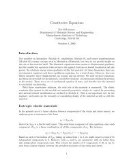
Using the steepest descent algorithm to minimize f (x) starting from
1 1
x 1 =(x 1 ,x 2 )=(0, 10), and using a tolerance of ɛ = 10 −6 , we compute the
iterates shown in Table 2 and in Figure 2:
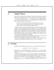
For a convex quadratic function f (x) = 1 x T Qx−c T x, the contours of the
2
function values will be shaped like ellipsoids, and the gradient vector ∇f (x)
at any point x will be perpendicular to the contour line passing through x,
see Figure 1.
8

k
x k
1 x k
2
k
d 1
k
d 2 ||d k || 2 α k f (x k )
1 0.000000 10.000000 −26.000000 −14.000000 29.52964612 0.0866 60.000000
2 −2.252782 8.786963 1.379968 −2.562798 2.91071234 2.1800 22.222576
3 0.755548 3.200064 −6.355739 −3.422321 7.21856659 0.0866 12.987827
4 0.204852 2.903535 0.337335 −0.626480 0.71152803 2.1800 10.730379
5 0.940243 1.537809 −1.553670 −0.836592 1.76458951 0.0866 10.178542
6 0.805625 1.465322 0.082462 −0.153144 0.17393410 2.1800 10.043645
7 0.985392 1.131468 −0.379797 −0.204506 0.43135657 0.0866 10.010669
8 0.952485 1.113749 0.020158 −0.037436 0.04251845 2.1800 10.002608
9 0.996429 1.032138 −0.092842 −0.049992 0.10544577 0.0866 10.000638
10 0.988385 1.027806 0.004928 −0.009151 0.01039370 2.1800 10.000156
11 0.999127 1.007856 −0.022695 −0.012221 0.02577638 0.0866 10.000038
12 0.997161 1.006797 0.001205 −0.002237 0.00254076 2.1800 10.000009
13 0.999787 1.001920 −0.005548 −0.002987 0.00630107 0.0866 10.000002
14 0.999306 1.001662 0.000294 −0.000547 0.00062109 2.1800 10.000001
15 0.999948 1.000469 −0.001356 −0.000730 0.00154031 0.0866 10.000000
16 0.999830 1.000406 0.000072 −0.000134 0.00015183 2.1800 10.000000
17 0.999987 1.000115 −0.000332 −0.000179 0.00037653 0.0866 10.000000
18 0.999959 1.000099 0.000018 −0.000033 0.00003711 2.1800 10.000000
19 0.999997 1.000028 −0.000081 −0.000044 0.00009204 0.0866 10.000000
20 0.999990 1.000024 0.000004 −0.000008 0.00000907 2.1803 10.000000
21 0.999999 1.000007 −0.000020 −0.000011 0.00002250 0.0866 10.000000
22 0.999998 1.000006 0.000001 −0.000002 0.00000222 2.1817 10.000000
23 1.000000 1.000002 −0.000005 −0.000003 0.00000550 0.0866 10.000000
24 0.999999 1.000001 0.000000 −0.000000 0.00000054 0.0000 10.000000
Table 2: Iterations of the example in Subsection 4.1.
9

5 x 2 +4 y 2 +3 x y+7 x+20
1200
1000
800
600
400
200
0
10
5
y
0
−5
−10
−10
−5
x
0
5
10
Figure 1: The contours of a convex quadratic function are ellipsoids.
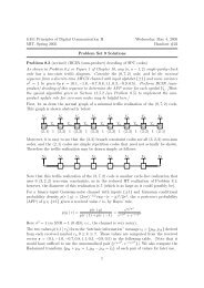
4.2 Example 2: Hem-Stitching
Consider the function
f(x) = 1 2 xT Qx − c T x +10
where Q and c are given by:
and
Q =
c =
(
20 5
5 2
(
14
6
)
)
10

10
8
6
4
2
0
−2
−5 0 5
Figure 2: Behavior of the steepest descent algorithm for the example of
Subsection 4.1.
A
For this problem, a
=30.234, and so the linear convergence rate δ of
(
A/a−1 ) 2
the steepest descent algorithm is bounded above by δ =
A/a+1
=0.8760.
If we apply the steepest descent algorithm to minimize f (x) starting
from x 1 =(40, −100), we obtain the iteration values shown in Table 3 and
shown graphically in Figure 3.
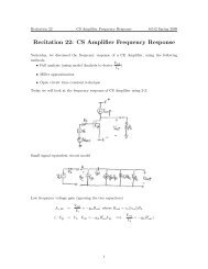
4.3 Example 3: Rapid Convergence
Consider the function
f (x) = 1 x T Qx − c T x +10
2
11

k
x k
1 x k
2 ||d k || 2 α k f (x k )
f (x k )−f (x ∗ )
f (x k−1 )−f (x ∗ )
1 40.000000 −100.000000 286.06293014 0.0506 6050.000000
2 25.542693 −99.696700 77.69702948 0.4509 3981.695128 0.658079
3 26.277558 −64.668130 188.25191488 0.0506 2620.587793 0.658079
4 16.763512 −64.468535 51.13075844 0.4509 1724.872077 0.658079
5 17.247111 −41.416980 123.88457127 0.0506 1135.420663 0.658079
6 10.986120 −41.285630 33.64806192 0.4509 747.515255 0.658079
7 11.304366 −26.115894 81.52579489 0.0506 492.242977 0.658079
8 7.184142 −26.029455 22.14307211 0.4509 324.253734 0.658079
9 7.393573 −16.046575 53.65038732 0.0506 213.703595 0.658079
10 4.682141 −15.989692 14.57188362 0.4509 140.952906 0.658079
20 0.460997 0.948466 1.79847660 0.4509 3.066216 0.658079
30 −0.059980 3.038991 0.22196980 0.4509 0.965823 0.658079
40 −0.124280 3.297005 0.02739574 0.4509 0.933828 0.658079
50 −0.132216 3.328850 0.00338121 0.4509 0.933341 0.658079
60 −0.133195 3.332780 0.00041731 0.4509 0.933333 0.658078
70 −0.133316 3.333265 0.00005151 0.4509 0.933333 0.658025
80 −0.133331 3.333325 0.00000636 0.4509 0.933333 0.654656
90 −0.133333 3.333332 0.00000078 0.0000 0.933333 0.000000
Table 3: Iteration values for example of Subsection 4.2, which shows hemstitching.
where Q and c are given by:
( )
20 5
Q =
5 16
and ( )
14
c =
6
A
For this problem, a
=1.8541, and so the linear convergence rate δ of
( )
A 2
−1 a
the steepest descent algorithm is bounded above by δ = =0.0896.
A
+1 a
12

Figure 3: Hem-stitching in the example of Subsection 4.2.
If we apply the steepest descent algorithm to minimize f (x) starting
from x 1 =(40, −100), we obtain the iteration values shown in Table 4 and
shown graphically in Figure 4.
Figure 4: Rapid convergence in the example of Subsection 4.3.
13

k
x k
1 x k
2 ||d k || 2 α k f (x k )
f (x k )−f (x ∗ )
f (x k−1 )−f (x ∗ )
1 40.000000 −100.000000 1434.79336491 0.0704 76050.000000
2 19.867118 −1.025060 385.96252652 0.0459 3591.615327 0.047166
3 2.513241 −4.555081 67.67315150 0.0704 174.058930 0.047166
4 1.563658 0.113150 18.20422450 0.0459 12.867208 0.047166
5 0.745149 −0.053347 3.19185713 0.0704 5.264475 0.047166
6 0.700361 0.166834 0.85861649 0.0459 4.905886 0.047166
7 0.661755 0.158981 0.15054644 0.0704 4.888973 0.047166
8 0.659643 0.169366 0.04049732 0.0459 4.888175 0.047166
9 0.657822 0.168996 0.00710064 0.0704 4.888137 0.047166
10 0.657722 0.169486 0.00191009 0.0459 4.888136 0.047166
11 0.657636 0.169468 0.00033491 0.0704 4.888136 0.047166
12 0.657632 0.169491 0.00009009 0.0459 4.888136 0.047161
13 0.657628 0.169490 0.00001580 0.0704 4.888136 0.047068
14 0.657627 0.169492 0.00000425 0.0459 4.888136 0.045002
15 0.657627 0.169491 0.00000075 0.0000 4.888136 0.000000
Table 4: Iteration values for the example in Subsection 4.3, which exhibits
rapid convergence.
4.4 Example 4: A nonquadratic function
Let
∑ 4 ∑ 4
f (x) = x 1 − 0.6x 2 +4x 3 +0.25x 4 − log(x i ) − log(5 − x i ) .
i=1 i=1
Table 5 shows values of the iterates of steepest descent applied to this
function.
4.5 Example 5: An analytic example
Suppose that
f (x) = 1 x T Qx + q T x
2
14

k
x k
1 x k
2 x k
3 x k
4 ||d k || 2 f (x k )
f (x k )−f (x ∗ )
f (x k−1 )−f (x ∗ )
1 1.000000 1.000000 1.000000 1.000000 4.17402683 4.650000
2 0.802973 1.118216 0.211893 0.950743 1.06742574 2.276855 0.219505
3 0.634501 1.710704 0.332224 1.121308 1.88344095 1.939389 0.494371
4 0.616707 1.735137 0.205759 1.108079 0.46928947 1.797957 0.571354
5 0.545466 1.972851 0.267358 1.054072 1.15992055 1.739209 0.688369
6 0.543856 1.986648 0.204195 1.044882 0.31575186 1.698071 0.682999
7 0.553037 2.121519 0.241186 0.991524 0.80724427 1.674964 0.739299
8 0.547600 2.129461 0.202091 0.983563 0.23764416 1.657486 0.733266
9 0.526273 2.205845 0.229776 0.938380 0.58321024 1.646479 0.770919
10 0.525822 2.212935 0.202342 0.933770 0.18499125 1.637766 0.764765
20 0.511244 2.406747 0.200739 0.841546 0.06214411 1.612480 0.803953
30 0.503892 2.468138 0.200271 0.813922 0.02150306 1.609795 0.806953
40 0.501351 2.489042 0.200095 0.804762 0.00743136 1.609480 0.807905
50 0.500467 2.496222 0.200033 0.801639 0.00256658 1.609443 0.808228
60 0.500161 2.498696 0.200011 0.800565 0.00088621 1.609439 0.808338
70 0.500056 2.499550 0.200004 0.800195 0.00030597 1.609438 0.808376
80 0.500019 2.499845 0.200001 0.800067 0.00010564 1.609438 0.808381
90 0.500007 2.499946 0.200000 0.800023 0.00003647 1.609438 0.808271
100 0.500002 2.499981 0.200000 0.800008 0.00001257 1.609438 0.806288
110 0.500001 2.499993 0.200000 0.800003 0.00000448 1.609438 0.813620
120 0.500000 2.499998 0.200000 0.800001 0.00000145 1.609438 0.606005
121 0.500000 2.499998 0.200000 0.800001 0.00000455 1.609438 0.468218
122 0.500000 2.499998 0.200000 0.800001 0.00000098 1.609438 0.000000
Table 5: Iteration values for the example of Subsection 4.4.
15

where ( ) ( )
+4 −2 +2
Q =
and q = .
−2 +2
−2
Then ( )( ) ( )
+4 −2 x +2
∇f (x) =
1
+
−2 +2 x 2 −2
and so ( )
∗ 0
x =
1
and
f (x ∗ )= −1.
√
Direct computation
√
shows that the eigenvalues of Q are A =3 + 5and
a = 3 − 5, whereby the bound on the convergence constant is
(
A/a − 1 ) 2
δ = ≤ 0.556.
A/a +1
Suppose that x 0 =(0, 0). Then we have:
x 1 =(−0.4, 0.4), x 2 =(0, 0.8)
and the even numbered iterates satisfy
x 2n =(0, 1 − 0.2 n ) and f (x 2n )=(1 − 0.2 n ) 2 − 2 + 2(0.2) n
and so
∗
f (x 2n ) − f (x )=(0.2) 2n .
Therefore, starting from the point x 0 =(0, 0), the optimality gap goes down
by a factor of 0.04 after every two iterations of the algorithm.
5 Final
Remarks
• The proof of convergence is basic in that it only relies on fundamental
properties of the continuity of the gradient and on the closedness and
boundedness of the level sets of the function f (x).
• The analysis of the rate of convergence is quite elegant.
16

• Kantorovich won the Nobel Prize in Economics in 1975 for his contributions
to the application of linear programming to economic theory.
• The bound on the rate of convergence is attained in practice quite
often, which is too bad.
• The ratio of the largest to the smallest eigenvalue of a matrix is called
the condition number of the matrix. The condition number plays an
extremely important role in the theory and the computation of quantities
involving the matrix Q.
• What about non-quadratic functions Most functions behave as nearquadratic
functions in a neighborhood of the optimal solution. The
analysis of the non-quadratic case gets very involved; fortunately, the
key intuition is obtained by analyzing the quadratic case.
6 A Bisection Algorithm for a Line-Search of a
Convex Function
Suppose that f(x) is a continuously differentiable convex function, and that
we seek to solve:
α ¯ := arg min f(¯ x + αd¯),
′
α
where ¯x is our current iterate, and d¯is the current direction generated by an
algorithm that seeks to minimize f(x). Suppose further that d¯ is a descent
direction of f(x) at x =¯, x namely:
Let
f(¯ x + ɛd¯) < f(¯ x) for all ɛ >0 and sufficiently small .
h(α) := f(¯x + αd¯),
whereby h(α) is a convex function in the scalar variable α, and our problem
is to solve for
ᾱ =arg min h(α).
α
We therefore seek a value ᾱ for which
h (ᾱ) =0.
17

It is elementary to show that
Proposition 6.1 h ′ (0) < 0.
q.e.d.
′
h (α) = ∇f (¯ x + αd) ¯ T d. ¯
Because h(α) is a convex function of α, wealsohave:
Proposition 6.2 h ′ (α) is a monotone increasing function α. of
q.e.d.
Figure 5 shows an example of convex function of two variables to be
optimized. Figure 6 shows the function h(α) obtained by restricting the
function of Figure 5 to the line shown in that figure. Note from Figure 6 that
h(α) is convex. Therefore its first derivative h ′ (α) will be a monotonically
increasing function. This is shown in Figure 7.
Because h ′ (α) is a monotonically increasing function, we can approxiα,
¯ the point that satisfies h ′ (¯ α) = 0, by a suitable bisection
mately compute
method. Suppose that we know a value α ˆ that h ′ (ˆ α) > 0. Since h ′ (0) < 0
and h ′ (ˆ α) > 0, the mid-value α ˜ = 0+ 2α ˆ is a suitable test-point. Note the
following:
• If h ′ (˜α) = 0, we are done.
• If h ′ (˜ α) > 0, we can now bracket α ¯ in the interval (0, α). ˜
• If h ′ (˜ α) < 0, we can now bracket α ¯ in the interval ( α, ˜ α). ˆ
This leads to the following bisection algorithm for minimizing h(α) = f (¯x +
¯ αd) by solving the equation h ′ (α) ≈ 0.
Step 0. Set k = 0. Set α l := 0 and α u := ˆα.
α = αu+α l
Step k. Set ˜ and compute h ′ 2
(˜ α).
18

20
10
0
−10
−20
f(x ,x−30)
1 2
−40
−50
−60
−70
−80
0
0.5
1
x 2
1.5
2
2.5
3 −2
0
2
4
x 1
6
8
10
Figure 5: A convex function to be optimized.
19

0
−10
−20
h(α)
−30
−40
−50
−60
−0.4 −0.2 0 0.2 0.4 0.6 0.8 1
α
Figure 6: The 1-dimensional function h(α).
1
0.5
0
h′(α)
−0.5
−1
−1.5
−2
−0.4 −0.2 0 0.2 0.4 0.6 0.8 1
α
Figure 7: The function h ′ (α) is monotonically increasing.
20

• If h ′ (˜ α) > 0, re-set α u := α. ˜ Set k ← k +1.
• If h ′ (˜ α) < 0, re-set α l := α. ˜ Set k ← k +1.
• If h ′ (˜α) = 0, stop.
Proposition 6.3 After every iteration of the bisection algorithm, the current
interval [α l ,α u ] must contain a point α ¯ such that h ′ (¯ α) =0.
Proposition 6.4 At the k th iteration of the bisection algorithm, the length
of the current interval [α l ,α u ] is
( )
1 k
L = (ˆα).
2
Proposition 6.5 A value of α such that |α − ᾱ| ≤ɛ canbefoundinat
most ⌈ ( )⌉
ˆα
log 2
ɛ
steps of the bisection algorithm.
6.1 Computing α for which h (ˆ
′
ˆ α) > 0
Suppose that we do not have available a convenient value αˆ for which h ′ (ˆ α) >
0. One way to proceed is to pick an initial “guess” of α ˆ and compute h ′ (ˆ α).
If h ′ (ˆ α) > 0, then proceed to the bisection algorithm; if h ′ (ˆ α) ≤ 0, then
re-set α ˆ ← 2ˆ α and repeat the process.
6.2 Stopping Criteria for the Bisection Algorithm
In practice, we need to run the bisection algorithm with a stopping criterion.
Some relevant stopping criteria are:
• Stop after a fixed number of iterations. That is stop when k = K, ¯
where K ¯ specified by the user.
• Stop when the interval becomes small. That is, stop when α u −α l ≤ ɛ,
where ɛ is specified by the user.
• Stop when |h ′ (˜ α)| becomes small. That is, stop when |h ′ (˜ α)| ≤ɛ,
where ɛ is specified by the user.
This third stopping criterion typically yields the best results in practice.
21

6.3 Modification of the Bisection Algorithm when the Domain
of f (x) is Restricted
The discussion and analysis of the bisection algorithm has presumed that
our optimization problem is
P : minimize f (x)
n
s.t. x ∈ R .
Given a point ¯x and a direction d¯, the line-search problem then is
LS : minimize h(α) := f (¯x + αd¯)
s.t. α ∈ R.
n
Suppose instead that the domain of definition of f (x) isanopenset X ⊂ R .
Then our optimization problem is:
P : minimize f (x)
s.t. x ∈ X,
and the line-search problem then is
LS : minimize h(α) := f (¯x + αd¯)
s.t. x ¯ + αd ¯∈ X.
In this case, we must ensure that all iterate values of α in the bisection alx
¯ + αd ¯ ∈ X. As an example, consider the following gorithm satisfy problem:
∑ m
P : minimize f (x) := − ln(b i − A i x)
i=1
s.t. b − Ax > 0.
22

Here the domain of f(x) is X = {x ∈R | b − Ax > 0}. Given
¯x ∈ X and a direction d¯, the line-search problem is:
n
a
point
∑
LS : minimize h(α) := f(¯ x + αd¯) = − m ln(b i − A i (¯ x + αd¯))
i=1
s.t. b − A(¯x + αd¯) > 0.
Standard arithmetic manipulation can be used to establish that
b − A(¯ x + αd¯) > 0 if and only if α

7 Proof of Kantorovich Inequality
Kantorovich Inequality: Let A and a be the largest and the smallest
eigenvalues of Q, respectively. Then
(A + a) 2
β ≤ .
4Aa
Proof: Let Q = RDR T , and then Q −1 = RD −1 R T , where R = R T is
an orthonormal matrix, and the eigenvalues of Q are
0 < a = a 1 ≤ a 2 ≤ ... ≤ a n = A,
and,
⎛ ⎞
a1 0 ... 0
0 a 2 ... 0 D = ⎜
⎝
.
. . .
⎟ . . ⎠ .
0 0 ... a n
Then
β =
(d T RDR T d)(d T RD −1 R T d) f T Dff T D −1 f
=
(d T RR T d)(d T RR T d) f T ff T f
∑ n
where f = R T f
d.Let λ i = f T i 2
f . Then λ i ≥ 0and
λ i =1, and
i=1
∑ n ( )
1
∑n
∑ n ( ) λ
1 i a i
i=1
β = λ i a i λ i = ⎛ ⎞ .
a
i=1 i=1 i
⎜ 1 ⎟
⎝ ∑ n ⎠
λ i a i
i=1
The largest value of β is when λ 1 + λ n = 1, see the illustration in Figure 8.
Therefore,
24

1 1
λ 1 a
+ λ n A
= (λ 1a + λ n A)(λ 1 A + λ n a) ( 1 A + 1 a)( 1 a + 1 A) ≤
2 2 2 2
(A + a) 2
β ≤
1 = .
Aa Aa 4Aa
q.e.d.
λ 1 a+λ nA
y
y = 1/x
Σλ i
(1/a i
)
1/(Σλ i
a i
)
0
Σλ i
a i
0 a 1 a 2
a 3 . . . a n
x
=a =A
Figure 8: Illustration for proof of the Kantorovich Inequality.
25

8 Steepest Descent Exercises
NOTE ON COMPUTATION EXERCISES: You may use any machine
and any programming language. We recommend, however, that you use
MATLAB on Athena or on your own computer. (The teaching assistant
is prepared to help you get started in MATLAB on Athena.) Some of the
specific details in the computation exercises are purposely left to your own
discretion. For example, in cases where you must use a line-search routine,
you must choose your own tolerance for the line-search. Also, you must
choose your own stopping criteria for your computation. Please include
your code or pseudo-code in your write-up.
1. (Steepest Descent) Suppose that x k and x k+1 are two consecutive
points generated by the steepest descent algorithm with exact linesearch.
Show that ∇f(x k ) T ∇f(x k+1 )=0.
2. (Steepest Descent) Suppose that we seek to minimize
2 2
f(x 1 ,x 2 )=5x +5x 2 − x 1 x 2 − 11x 1 +11x 2 +11.
1
(a) Find a point satisfying the first-order necessary conditions for a
solution.
(b) Show that this point is a global minimum of f(x).
(c) What would be the worst rate of convergence for the steepest
descent algorithm for this problem
(d) Starting at (x 1 ,x 2 )=(0, 0), at most how many steepest descent
iterations would it take to reduce the function value to 10 −11
3. (Steepest Descent) Suppose we seek to minimize
1 T
f(x) = x T Hx + c x +13,
2
where ( ) ( )
10 −9 4
H =
and c = .
−9 10
−15
Implement the steepest descent algorithm on this problem, using the
following starting points:
26

• x 0 =(0, 0) T .
• x 0 =(−0.4, 0) T .
• x 0 =(10, 0) T .
• x 0 =(11, 0) T .
As it turns out, the optimal solution to this problem is x =(5, 6) T ,
∗
with f(x )= −22. What linear convergence constants do you observe
for each of the above starting points
4. (Steepest Descent) Suppose we seek to minimize
1 T
f(x) = x T Hx + c x,
2
where ⎛ ⎞ ⎛ ⎞
10 −18 2 12
⎜ ⎟ ⎜ ⎟
H = ⎝ −18 40 −1 ⎠ and c = ⎝ −47 ⎠ .
2 −1 3 −8
Implement the steepest descent algorithm on this problem, using the
following starting points.
• x 0 =(0, 0, 0) T .
• x 0 =(15.09, 7.66, −6.56) T .
• x 0 =(11.77, 6.42, −4.28) T .
• x 0 =(4.46, 2.25, 1.85) T .
As it turns out, the optimal solution to this problem is x =(4, 3, 1) T ,
∗
with f(x )= −50.5. What linear convergence constants do you observe
for each of the above starting points
5. (Steepest Descent) Suppose that we seek to minimize the following
function:
f(x 1 ,x 2 )= −9x 1 −10x 2 +θ(− ln(100−x 1 −x 2 )−ln(x 1 )−ln(x 2 )−ln(50−x 1 +x 2 )),
where θ is a given parameter. Note that the domain of this function
is X = {(x 1 ,x 2 ) | x 1 > 0,x 2 > 0,x 1 + x 2 < 100,x 1 − x 2 < 50}.
Implement the steepest descent algorithm for this problem, using the
∗
∗
27

isection algorithm for your line-search, with the stopping criterion
that |h ′ (˜α)| ≤ ɛ = 10 −6 . Run your algorithm for θ = 10 and for
θ = 100, using the following starting points.
• x 0 =(8, 90) T .
• x 0 =(1, 40) T .
• x 0 =(15, 68.69) T .
• x 0 =(10, 20) T .
What linear convergence constants do you observe for each of the above
starting points
Helpful Hint: Note that f(x 1 ,x 2 ) is only defined on the domain
X = {(x 1 ,x 2 ) | x 1 > 0,x 2 > 0,x 1 + x 2 < 100,x 1 −x 2 < 50}. If you are
at a point x ¯ = (¯ x 1 , x¯ 2 ) and you have computed a direction d ¯= (d¯ 1 , d¯
2 ),
then note that a value of the upper bound ˆα is effectively given by the
largest value of α for which the following constraints are satisfied:
x¯ 1 +αd¯ 1 > 0, x¯ 2 +αd¯ 2 > 0, x¯ 1 +αd¯ 1+¯ x 2 +αd¯ ¯ ¯ ¯ ¯
2 < 100, x 1 +αd 1 −x 2 −αd 2 < 50.
The largest value of α satisfying these conditions can easily be computed
by applying appropriate logic.
Important Note: Please keep the value of θ as a specific command
in your code. The reason for this is that later in the semester, we will
consider an algorithm where we iteratively change the value of θ. It
will then be useful for your code to have a line in it where θ can be
set and re-set.
28