Chapter 4 Vector-Valued Functions
Chapter 4 Vector-Valued Functions
Chapter 4 Vector-Valued Functions

You also want an ePaper? Increase the reach of your titles
YUMPU automatically turns print PDFs into web optimized ePapers that Google loves.
<strong>Chapter</strong> 4<br />
<strong>Vector</strong>-<strong>Valued</strong> <strong>Functions</strong><br />
4.1 Introduction to <strong>Vector</strong>-<strong>Valued</strong> <strong>Functions</strong><br />
Parametric Curves in 3-Space<br />
Recall that if f and g are well-behaved functions, then the pair of parametric equations<br />
x = f(t), y = g(t) (4.1)<br />
generatesacurve in2-spacethatistracedinaspecific directionastheparameter tincreases.<br />
We define this direction to be the orientation of the curve or the direction of increasing<br />
parameter, and we called the curve together with its orientation the graph of the parametric<br />
equations or the parametric curve represented by the equations. Analogously, if f, g and h<br />
are three well-behaved functions, then the parametric equations<br />
x = f(t), y = g(t), z = h(t) (4.2)<br />
generatesacurve in3-spacethatistracedinaspecificdirectionastincreases. Asin2-space,<br />
this direction is called the orientation or direction of increasing parameter, and the<br />
curve together with its orientation is called the graph of the parametric equations or the<br />
parametric curve represented by the equations. If no restrictions are state explicitly<br />
or are implied by the equation, then it will be understood that t varies over the interval<br />
(−∞,+∞).<br />
Example 4.1 Describe the parametric curve represented by the equations<br />
Solution .........<br />
x = 1−t, y = 3t, z = 2t.<br />
Example 4.2 Describe the parametric curve represented by the equations<br />
where a and c are positive constants.<br />
x = acosθ, y = asinθ, z = ct.<br />
62
MA112 Section 750001: Prepared by Dr.Archara Pacheenburawana 63<br />
Solution As the parameter t increases, the value of z = ct also increases, so the point<br />
(x,y,z) moves upward. However, as t increases, the point (x,y,z) also moves in a path<br />
directly over the circle<br />
x = acosθ, y = asinθ<br />
in the xy-plane. The combination of these upward and circular motions produces a cork<br />
screw-shaped curve that wraps around a right circular cylinder of radius a centered on the<br />
z-axis. This curve is called a circular helix.<br />
z<br />
x<br />
y<br />
✠<br />
Parametric Equations for Intersections of Surfaces<br />
Curve in 3-space often arise as intersections of surfaces. One method for finding parametric<br />
equations for the curve of intersection is to choose one of the variables as the parameter and<br />
use the two equations to express the remaining two variables in terms of that parameter.<br />
For example, suppose we want to find parametric equations of the intersection of the<br />
cylinder z = x 3 and y = x 2 . We choose x = t as the parameter and substitute this into the<br />
equations z = x 3 and y = x 2 , then we obtain the parametric equations<br />
This curve is called a twisted cubic.<br />
x = t, y = t 2 , z = t 3 (4.3)
MA112 Section 750001: Prepared by Dr.Archara Pacheenburawana 64<br />
<strong>Vector</strong>-<strong>Valued</strong> <strong>Functions</strong><br />
The twisted cubic defined by the equations in (4.3) is the set of points of the form (t,t 2 ,t 3 )<br />
for real values of t. If we view each of these points as a terminal point for a vector r whose<br />
initial point is at the origin,<br />
r = 〈x,y,z〉 = 〈t,t 2 ,t 3 〉 = ti+t 2 j+t 2 k<br />
then we obtain r as a function of the parameter t, that is, r = r(t). Since this function<br />
produces a vector, we say that r = r(t) defines r as a vector-valued function of a real<br />
variable, or more simply, a vector-valued function.<br />
If r(t) is a vector-valued function in 2-space, then for each allowable value of t the vector<br />
r = r(t) can be represented in terms of components as<br />
r = r(t) = 〈x(t),y(t)〉 = x(t)i+y(t)j<br />
The functions x(t) and y(t) are called the component functions or the components of<br />
r(t). Similarly, the component functions of a vector-valued function<br />
in 3-space are x(t), y(t) and z(t).<br />
r = r(t) = 〈x(t),y(t),z(t)〉 = x(t)i+y(t)j+z(t)k<br />
Example 4.3 The component functions of<br />
are<br />
r(t) = 〈t,t 2 ,t 3 〉 = ti+t 2 j+t 3 k<br />
x(t) = t, y(t) = t 2 , z(t) = t 3<br />
The domain of a vector-valued function r(t) is the set of allowable values for t. If r(t)<br />
is defined in terms of component functions and the domain is not specified explicitly, then<br />
the domain is the intersection of the natural domains of the component functions; this is<br />
called the natural domain of r(t).<br />
Example 4.4 Find the natural domain of<br />
Solution .........<br />
r(t) = 〈ln|t−1|,e t , √ t〉 = (ln|t−1|)i+e t j+ √ tk<br />
Graphs of <strong>Vector</strong>-<strong>Valued</strong> <strong>Functions</strong><br />
If r(t) is a vector-valued function in 2-space or 3-space, then we define the graph of r(t) to<br />
be the parametric curve described by the component functions for r(t).<br />
For example, if<br />
r(t) = 〈1−t,3t,2t〉 = (1−t)i+3tj+2tk (4.4)<br />
then the graph of r = r(t) is the graph of the parametric equations<br />
x = 1−t, y = 3t, z = 2t<br />
Thus, the graph of (4.4) is the line in Example 4.1.<br />
✠
•<br />
MA112 Section 750001: Prepared by Dr.Archara Pacheenburawana 65<br />
Example 4.5 Describe the graph of the vector-valued function<br />
Solution .........<br />
r(t) = 〈cost,sint,t〉 = costi+sintj+tk<br />
If a parametric curve is viewed as the graph of a vector-valued function, then we can<br />
also imagine the graph to be traced by the tip of the moving vector. For example, if the<br />
curve C in 3-space is the graph of<br />
r(t) = x(t)i+y(t)j+z(t)k<br />
and if we position r(t) so its initial point is at the origin, then its terminal point will fall<br />
on the curve C.<br />
z<br />
(x(t),y(t),z(t))<br />
r(t)<br />
C<br />
y<br />
x<br />
Thus, when r(t) is positioned with its initial point at the origin, its terminal point will trace<br />
out the curve C as the parameter t varies, in which case we call r(t) the radius vector or<br />
the position vector for C.<br />
Example 4.6 Sketch the graph and a radius vector of<br />
(a) r(t) = costi+sintj, 0 ≤ t ≤ 2π<br />
(b) r(t) = costi+sintj+2k, 0 ≤ t ≤ 2π<br />
Solution .........<br />
<strong>Vector</strong> Form of a Line Segment<br />
Recall that if r 0 is a vector in 2-space or 3-space with its initial points at the origin, then<br />
the line that passes through the terminal point of r 0 and is parallel to the vector v can be<br />
expressed in vector form as<br />
r = r 0 +tv<br />
In particular, if r 0 and r 1 are vectors in 2-space or 3-space with their initial points at<br />
the origin, then the line that passes through the terminal points of these vectors can be<br />
expressed in vector form as<br />
r = r 0 +t(r 1 −r 0 ) or r = (1−t)r 0 +tr 1 (4.5)
•<br />
•<br />
•<br />
•<br />
MA112 Section 750001: Prepared by Dr.Archara Pacheenburawana 66<br />
r 0<br />
t(r 1 −r 0 )<br />
r<br />
O<br />
r 1<br />
r = (1−t)r 0 +tr 1<br />
It is common to call (4.5) the two-point vector form of a line. It is understood<br />
in (4.5) that t varies from −∞ to +∞. However, if we restrict t to vary over the interval<br />
0 ≤ t ≤ 1, then r will vary from r 0 to r 1 . Thus, the equation<br />
r = (1−t)r 0 +tr 1 (0 ≤ t ≤ 1) (4.6)<br />
represents the line segment in 2-space or 3-space that is traced from r 0 to r 1 .<br />
4.2 Calculus of <strong>Vector</strong>-<strong>Valued</strong> <strong>Functions</strong><br />
In this section we will define limits, derivative, and integral of vector-valued functions.<br />
Limits and Continuity<br />
Our first goal in this section is to develop a notion of what it means for a vector-valued<br />
function r(t) in 2-space or 3-space to approach a limiting vector L ar t approaches a number<br />
a. That is, we want to define<br />
limr(t) = L (4.7)<br />
t→a<br />
Definition 4.1 Let r(t) be a vector-valued function that is defined for all t in some open<br />
interval containing the number a, except that r(t) need not be defined at a. We will write<br />
limr(t) = L<br />
t→a<br />
if and only if<br />
Theorem 4.1<br />
lim‖r(t)−L‖ = 0<br />
t→a<br />
(a) If r(t) = 〈x(t),y(t)〉 = x(t)i+y(t)j, then<br />
limr(t) =<br />
t→a<br />
〈<br />
lim<br />
t→a<br />
x(t),lim<br />
t→a<br />
y(t)<br />
〉<br />
= lim<br />
t→a<br />
x(t)i+lim<br />
t→a<br />
y(t)j<br />
provided the limits of the component functions exist. Conversely, the limits of the<br />
component functions exist provided r(t) approaches a limiting vector as t approaches<br />
a.
MA112 Section 750001: Prepared by Dr.Archara Pacheenburawana 67<br />
(b) If r(t) = 〈x(t),y(t),z(t)〉 = x(t)i+y(t)j+z(t)k, then<br />
〈<br />
〉<br />
limr(t) = limx(t),limy(t),limz(t)<br />
t→a t→a t→a t→a<br />
= lim<br />
t→a<br />
x(t)i+lim<br />
t→a<br />
y(t)j+lim<br />
t→a<br />
z(t)k<br />
provided the limits of the component functions exist. Conversely, the limits of the<br />
component functions exist provided r(t) approaches a limiting vector as t approaches<br />
a.<br />
Example 4.7 Find lim<br />
t→0<br />
(<br />
(t 2 +1)i+5costj+sintk ) .<br />
Solution .........<br />
Example 4.8 Find lim<br />
t→0<br />
〈t 2 ,e t ,−2cosπt〉.<br />
Solution .........<br />
Motivated by the definition of continuity for real-valued functions, we define a vectorvalued<br />
function r(t) to be continuous at t = a if<br />
limr(t) = r(a) (4.8)<br />
t→a<br />
That is, r(a) is defined, the limit of r(t) as t → a exists, and the two are equal. As in the<br />
case for real-valued functions, we say that r(t) is continuous on an interval I if it is<br />
continuous at each point of I. It follows from Theorem 4.1 that a vector-valued function is<br />
continuous at t = a if and only if its component functions are continuous at t = a.<br />
Derivatives<br />
The derivative of a vector-valued function is defined by a limit similar to that for the<br />
derivative of a real-values function.<br />
Definition 4.2 If r(t) is a vector-valued function, we define the derivative of r with<br />
respect to t to be the vector-valued function r ′ given by<br />
r ′ (t) = lim<br />
h→0<br />
r(t+h)−r(t)<br />
h<br />
(4.9)<br />
The domain of r consists of all values of t in the domain of r(t) for which the limit exists.<br />
The function r(t) is differentiable at t if the limit in (4.9) exists. All of the standard<br />
notations for derivatives continue to apply. For example, the derivative of r(t) can be<br />
expressed as<br />
d<br />
dt [r(t)], dr<br />
dt , r′ (t), or r ′
•<br />
MA112 Section 750001: Prepared by Dr.Archara Pacheenburawana 68<br />
Geometric Interpretation of the Derivative.<br />
Suppose that C is the graph of a vector-valued function r(t) in 2-space or 3-space and that<br />
r ′ (t) exists and is nonzero for a given value of t. If the vector r ′ (t) is positioned with its<br />
initial point as the terminal point of the radius vector r(t), then r ′ (t) is tangent to C and<br />
points in the direction of increasing parameter.<br />
y<br />
r ′ (t)<br />
r(t)<br />
C<br />
x<br />
Theorem 4.2 If r(t) is a vector-valued function, then r is differentiable at t if and only if<br />
each of its component functions is differentiable at t, in which case the component functions<br />
of r ′ (t) are the derivatives of the corresponding component functions of r(t).<br />
Example 4.9 Find the derivative of r(t) = sin(t 2 )i+e cost j+tlntk.<br />
Solution .........<br />
Derivative Rules<br />
Many of the rules for differentiating real-valued functions have analogs in the context of<br />
differentiating vector-valued functions. We state some of these in the following theorem.<br />
Theorem 4.3 (Rules of Differentiation). Let r(t), r 1 (t), and r 2 (t) be vector-valued<br />
functions that are all in 2-space or all in 3-space, and let f(t) be a real-valued function, k a<br />
scalar, and c a constant vector (that is, a vector whose value does not depend on t). Then<br />
the following rules of differentiation hold:<br />
(a)<br />
(b)<br />
(c)<br />
(d)<br />
(c)<br />
d<br />
dt [c] = 0<br />
d<br />
dt [kr(t)] = k d dt [r(t)]<br />
d<br />
dt [r 1(t)+r 2 (t)] = d dt [r 1(t)]+ d dt [r 2(t)]<br />
d<br />
dt [r 1(t)−r 2 (t)] = d dt [r 1(t)]− d dt [r 2(t)]<br />
d<br />
dt [f(t)r(t)] = f(t) d dt [r(t)]+r(t) d dt [f(t)]
•<br />
MA112 Section 750001: Prepared by Dr.Archara Pacheenburawana 69<br />
Tangent Lines to Graphs of <strong>Vector</strong>-<strong>Valued</strong> <strong>Functions</strong><br />
Definition 4.3 Let P be a point on the graph of a vector-valued function r(t), and let r(t 0 )<br />
be the radius vector from the origin to P.<br />
y<br />
r ′ (t 0 )<br />
r(t 0 )<br />
P<br />
Tangent line<br />
x<br />
If r ′ (t 0 ) exists and r ′ (t 0 ) ≠ 0, then we call r ′ (t 0 ) a tangent vector to the graph of r(t) at<br />
r(t 0 ), and we call the line through P that is parallel to the tangent vector the tangent line<br />
to the graph of r(t) at r(t 0 ).<br />
Let r 0 = r(t 0 ) and v 0 = r ′ (t 0 ). Then the tangent line to the graph of r(t) at r 0 is given<br />
by the vector equation<br />
r = r 0 +tv 0 (4.10)<br />
Example 4.10 Find parametric equations of the tangent line to the circular helix<br />
x = cost, y = sint, z = t<br />
where t = t 0 , and use that result to find parametric equations for the tangent line at the<br />
point where t = π.<br />
Solution .........<br />
Example 4.11 Let<br />
and<br />
r 1 (t) = (tan −1 t)i+(sint)j+t 2 k<br />
r 2 (t) = (t 2 −t)i+(2t−2)j+(lnt)k<br />
The graphs of r 1 (t) and r 2 (t) intersect at the origin. Find the degree measure of the acute<br />
angle between the tangent lines to the graphs of r 1 (t) and r 2 (t) at the origin.<br />
Solution .........
MA112 Section 750001: Prepared by Dr.Archara Pacheenburawana 70<br />
Derivatives of Dot and Cross Products<br />
The following rules provide a method for differentiating dot products in 2-space and 3-space<br />
and cross product in 3-space.<br />
d<br />
dt [r 1(t)·r 2 (t)] = r 1 (t)· dr 2<br />
dt + dr 1<br />
dt ·r 2(t) (4.11)<br />
d<br />
dt [r 1(t)×r 2 (t)] = r 1 (t)× dr 2<br />
dt + dr 1<br />
dt ×r 2(t) (4.12)<br />
Theorem 4.4 If r(t) is a differentiable vector-valued function in 2-space or 3-space and<br />
‖r(t)‖ is constant for all t, then<br />
r(t)·r ′ (t) = 0 (4.13)<br />
that is, r(t) and r ′ (t) are orthogonal vectors for all t.<br />
Definite Integrals of <strong>Vector</strong>-<strong>Valued</strong> <strong>Functions</strong><br />
If r(t) is a vector-valued function that is continuous on the interval a ≤ t ≤ b, then we<br />
define the definite integral of r(t) over this interval as a limit of Riemann sums, that is,<br />
In general, we have<br />
∫ b<br />
a<br />
∫ b<br />
a<br />
(∫ b<br />
r(t)dt =<br />
∫ b<br />
a<br />
r(t)dt =<br />
(∫ b<br />
r(t)dt =<br />
a<br />
a<br />
lim<br />
max △t k →0<br />
n∑<br />
r(t ∗ k)△t k (4.14)<br />
k=1<br />
) (∫ b<br />
)<br />
x(t)dt i+ y(t)dt j 2-space (4.15)<br />
a<br />
) (∫ b<br />
) (∫ b<br />
)<br />
x(t)dt i+ y(t)dt j+ z(t)dt k 3-space (4.16)<br />
a<br />
a<br />
Example 4.12 Let r(t) = t 2 i+e t j−(2cosπt)k. Evaluate<br />
Solution .........<br />
∫ 1<br />
0<br />
r(t)dt.<br />
Rules of Integration<br />
As with differentiating, many of the rules for integrating real-values functions have analogs<br />
for vector-values functions.<br />
Theorem 4.5 (Rulesof Integration). Letr(t), r 1 (t), and r 2 (t) be vector-valued functions<br />
in 2-space or 3-space that are continuous on the interval a ≤ t ≤ b, and let k be a scalar.<br />
Then the following rules of integration hold:
MA112 Section 750001: Prepared by Dr.Archara Pacheenburawana 71<br />
(a)<br />
(b)<br />
(c)<br />
∫ b<br />
a<br />
∫ b<br />
a<br />
∫ b<br />
a<br />
∫ b<br />
kr(t)dt = k r(t)dt<br />
a<br />
[r 1 (t)+r 2 (t)]dt =<br />
[r 1 (t)−r 2 (t)]dt =<br />
∫ b<br />
a<br />
∫ b<br />
a<br />
r 1 (t)dt+<br />
r 1 (t)dt−<br />
∫ b<br />
a<br />
∫ b<br />
a<br />
r 2 (t)dt<br />
r 2 (t)dt<br />
Antiderivatives of <strong>Vector</strong>-<strong>Valued</strong> <strong>Functions</strong><br />
An antiderivative for a vector-valued function r(t) is a vector-valued function R(t) such<br />
that<br />
R ′ (t) = r(t) (4.17)<br />
We express Equation(4.17) using integral notation as<br />
∫<br />
r(t)dt = R(t)+C (4.18)<br />
where C represents an arbitrary constant vector. Note that the vector R(t) + C is also<br />
called the indefinite integral of r(t).<br />
Since differentiation of vector-valued functions can be performed componentwise, it follows<br />
that antidifferentiation can be done this way as well.<br />
∫<br />
Example 4.13 Evaluate the indefinite integral (2ti+3t 2 j+sin2tk)dt.<br />
Solution .........<br />
Mostofthefamiliarintegrationpropertieshavevector counterparts. Forexample, vector<br />
differentiation and integration are inverse operations in the sense that<br />
[∫<br />
d<br />
dt<br />
]<br />
r(t)dt = r(t) and<br />
∫<br />
r ′ (t)dt = r(t)+C (4.19)<br />
Moreover, if R(t) is an antiderivative of r(t) on an interval containing t = a and t = b, then<br />
we have the following vector form of the Fundamental Theorem of Calculus:<br />
∫ b<br />
a<br />
] b ∫<br />
r(t)dt = R(t) =<br />
a<br />
] b<br />
r(t)dt = R(b)−R(a) (4.20)<br />
a<br />
Example 4.14 Evaluate the definite integral<br />
Solution .........<br />
∫ 1<br />
0<br />
(<br />
sinπti+(6t 2 +4t)j ) dt.<br />
Example 4.15 Find r(t) given that r ′ (t) = 〈3,2t〉 and r(1) = 〈2,5〉.<br />
Solution .........
MA112 Section 750001: Prepared by Dr.Archara Pacheenburawana 72<br />
4.3 Change of Parameter; Arc Length<br />
We observed in earlier sections that a curve in 2-space or 3-space can be represented parametrically<br />
in more than one way. Sometimes it will be desirable to change the parameter for<br />
a parametric curve to a different parameter that is better suited for the problem at hand.<br />
Smooth Parametrizations<br />
A curve represented by r(t) is smoothly parametrized by r(t), that r(t) is a smooth<br />
function of t if r ′ (t) is continuous and r ′ (t) ≠ 0 for any allowable value of t. Geometrically,<br />
this means that the a smooth parametrized curve can have no abrupt changes in direction<br />
as the parameter increases.<br />
Example 4.16 Determine whether the following vector-valued functions are smooth.<br />
(a) r(t) = acosti+asintj+ctk (a > 0,c > 0)<br />
(b) r(t) = t 2 i+t 3 j<br />
Solution .........<br />
Arc Length from the <strong>Vector</strong> Viewpoint<br />
Recall that the arc length L of a parametric curve<br />
is given by the formula<br />
x = x(t), y = y(t) (a ≤ t ≤ b) (4.21)<br />
L =<br />
∫ b<br />
a<br />
√ (dx ) 2<br />
+<br />
dt<br />
Analogously, the arc length L of a parametric curve<br />
in 3-space is given by the formula<br />
( ) 2 dy<br />
dt (4.22)<br />
dt<br />
x = x(t), y = y(t), z = z(t) (a ≤ t ≤ b) (4.23)<br />
L =<br />
∫ b<br />
a<br />
√ (dx ) 2<br />
+<br />
dt<br />
( ) 2 dy<br />
+<br />
dt<br />
( ) 2 dz<br />
dt (4.24)<br />
dt<br />
Formulas (4.22) and (4.24) have vector forms that we can obtain by letting<br />
r(t) = x(t)i+y(t)j or r(t) = x(t)i+y(t)j+z(t)k<br />
It follows that<br />
dr<br />
dt = dx dy<br />
i+<br />
dt dt j or dr<br />
dt = dx dy dz<br />
i+ j+<br />
dt dt dt k
MA112 Section 750001: Prepared by Dr.Archara Pacheenburawana 73<br />
and hence<br />
√ (dx ) dr<br />
2 ∥dt∥ = +<br />
dt<br />
( ) 2 dy<br />
or<br />
dt<br />
√ (dx ) dr<br />
2 ∥dt∥ = +<br />
dt<br />
( ) 2 dy<br />
+<br />
dt<br />
( ) 2 dz<br />
dt<br />
Substituting these expressions in (4.22) and (4.24) leads us to the following theorem.<br />
Theorem 4.6 If C is the graph in 2-space or 3-space of a smooth vector-valued function<br />
r(t), then its arc length L from t = a to t = b is<br />
L =<br />
Example 4.17 Find the arc length of the vector-valued function<br />
from t = 0 to t = π.<br />
Solution .........<br />
∫ b<br />
a<br />
dr<br />
∥dt∥ dt (4.25)<br />
r(t) = costi+sintj+tk<br />
Example 4.18 Find the arc length of the vector-valued function<br />
Solution .........<br />
Arc Length as a Parameter<br />
r(t) = 〈2t,lnt,t 2 〉 for 1 ≤ t ≤ e.<br />
For many purpose the best parameter to use for representing a curve in 2-space or 3-space<br />
parametricallyisthelengthofarcmeasured alongthecurve fromsomefixed reference point.<br />
This can be done as follows:<br />
Using Arc Length as a Parameter<br />
Step 1. Select an arbitrary point on the curve C to serve as a reference point.<br />
Step 2. Starting from the reference point, choose one direction along the curve to be the<br />
positive direction and the other to be the negative direction.<br />
Step 3. If P is a point on the curve, let s be the signed arc length along C from the<br />
reference point to P, where s is positive if P is in the positive direction from the<br />
reference point and s is negative if P is in the negative direction.
•<br />
•<br />
•<br />
•<br />
•<br />
•<br />
•<br />
MA112 Section 750001: Prepared by Dr.Archara Pacheenburawana 74<br />
s = 3<br />
s = 2<br />
s = 1<br />
Reference point<br />
s = −1<br />
s = −2<br />
s = −3<br />
C<br />
Let us now treat s as a variable. As the value of s changes, the corresponding point<br />
P moves along C and the coordinate of P become functions of s. Thus, in 2-space the<br />
coordinate of P are (x(s),y(s)), and in 3-space they are (x(s),y(s),z(s)). Therefore in<br />
2-space or 3-space the curve C is given by the parametric equations<br />
x = x(s), y = y(s), or x = x(s), y = y(s), z = z(s)<br />
A parametric representation of a curve with arc length as the parameter is called an arc<br />
length parametrization of the curve.<br />
Example 4.19 Find the arc length parametrization of the circle x 2 + y 2 = a 2 with counterclockwise<br />
orientation and (a,0) as the reference point.<br />
Solution .........<br />
Change of Parameter<br />
A change of parameter in a vector-valued function r(t) is a substitution t = g(τ) that<br />
produce a new vector-valued function r(g(τ)) have the same graph as r(t), but possibly<br />
traced differently as the parameter τ increases.<br />
Example 4.20 Find a change of parameter t = g(τ) for the circle<br />
such that<br />
r(t) = costi+sintj (0 ≤ t ≤ 2π)<br />
(a) the circle is traced counterclockwise as τ increases over the interval [0,1];<br />
(b) the circle is traced clockwise as τ increases over the interval [0,1].<br />
Solution .........<br />
Theorem 4.7 (Chain Rule) Let r(t) be a vector-valued function in 2-space or 3-space<br />
that is differentiable with respect to t. If t = g(τ) is a change of parameter in which g is<br />
differentiable with respect to τ, then r((g(τ)) is differentiable with respect to τ and<br />
dr<br />
dτ = dr dt<br />
dt dτ<br />
(4.26)
•<br />
•<br />
MA112 Section 750001: Prepared by Dr.Archara Pacheenburawana 75<br />
A change of parameter t = g(τ) in which r(g(τ)) is smooth is called a smooth change<br />
of parameter. Smooth change of parameter fall into two categories—those for which<br />
dt/dτ > 0forallτ (calledpositive changes of parameter)andthoseforwhichdt/dτ < 0<br />
for all τ (called negative changes of parameter). A positive changes of parameter<br />
preserves theorientationofaparametriccurve, andanegativechangesofparameterreverses<br />
it.<br />
Finding Arc Length Parametrizations<br />
Theorem 4.8 Let C be the graph of a smooth vector-valued function r(t) in 2-space or 3-<br />
space, and let r 0 (t) be any point on C. Then the following formula defines a positive change<br />
of parameter from t to s, where s is an arc length parameter having r 0 (t) as its reference<br />
point:<br />
∫ t<br />
∥ ∥∥∥ dr<br />
s =<br />
t 0<br />
du∥ du (4.27)<br />
y<br />
r(t 0 )<br />
s<br />
r(t)<br />
C<br />
x<br />
When needed, Formula (4.27) can be expressed in component form as<br />
s =<br />
s =<br />
∫ t<br />
√ (dx ) 2<br />
+<br />
t 0<br />
du<br />
∫ t<br />
√ (dx ) 2<br />
+<br />
t 0<br />
du<br />
( ) 2 dy<br />
+<br />
du<br />
( ) 2 dy<br />
du 2-space (4.28)<br />
du<br />
( ) 2 dz<br />
du 3-space (4.29)<br />
du<br />
Example 4.21 Find the arc length parametrization of the circular helix<br />
r = costi+sintj+tk<br />
that has reference point r(0) = (1,0,0) and has the same orientation as the given helix.<br />
Solution .........<br />
Example 4.22 A bug walks along the trunk of a tree following a path modeled by the<br />
circular helix in Example 4.21. The bug starts at the reference point (1,0,0) and walks up<br />
the helix for a distance of 10 units. What are the bug’s final coordinates
MA112 Section 750001: Prepared by Dr.Archara Pacheenburawana 76<br />
Solution .........<br />
Example 4.23 Find the arc length parametrization of the line<br />
x = 2t+1, y = 3t−2<br />
that has the same orientation as the given line and uses (1,−2) as the reference point.<br />
Solution .........<br />
Properties of Arc Length Parametrizations<br />
Theorem 4.9<br />
(a) If C is the graph of a smooth vector-valued function r(t) in 2-space or 3-space, where<br />
t is a general parameter, and if s is the arc length parameter for C defined by Formula<br />
(4.27), then for every value of t the tangent vector has length<br />
dr<br />
∥dt∥ = ds<br />
(4.30)<br />
dt<br />
(b) If C is the graph of a smooth vector-valued function r(t) in 2-space or 3-space, where<br />
s is an arc length parameter, then for every value of s the tangent vector to C has<br />
length<br />
dr<br />
∥ds∥ = 1 (4.31)<br />
(c) If C is the graph of a smooth vector-valued function r(t) in 2-space or 3-space, and<br />
if ‖dr/dt‖ = 1 for every value of t, then for any value of t 0 in the domain of r, the<br />
parameter s = t−t 0 is an arc length parameter that has its reference point at the point<br />
on C where t = t 0 .<br />
The component forms of Formulas (4.30) and (4.31) are as follow:<br />
∥ √ (dx )<br />
ds ∥∥∥<br />
dt = dr<br />
2 dt∥ = +<br />
dt<br />
∥ √ (dx )<br />
ds ∥∥∥<br />
dt = dr<br />
2 dt∥ = +<br />
dt<br />
√ (dx ) dr<br />
2 ∥ds∥ = +<br />
ds<br />
√ (dx ) dr<br />
2 ∥ds∥ = +<br />
ds<br />
( ) 2 dy<br />
+<br />
ds<br />
( ) 2 dy<br />
+<br />
dt<br />
( ) 2 dy<br />
2-space (4.32)<br />
dt<br />
( ) 2 dz<br />
3-space (4.33)<br />
dt<br />
( ) 2 dy<br />
= 1 2-space (4.34)<br />
ds<br />
( ) 2 dz<br />
= 1 3-space (4.35)<br />
ds
MA112 Section 750001: Prepared by Dr.Archara Pacheenburawana 77<br />
4.4 Unit Tangent and Normal <strong>Vector</strong>s<br />
Unit Tangent <strong>Vector</strong>s<br />
Recall that if C is a graph of a smooth vector-valued function r(t) in 2-space or 3-space,<br />
then the vector r ′ (t) is nonzero, tangent to C, and points in the direction of increasing<br />
parameter. Thus, by normalizing r ′ (t) we obtain a unit vector<br />
T(t) = r′ (t)<br />
‖r ′ (t)‖<br />
(4.36)<br />
that is tangent to C and points in the direction of increasing parameter. We call T(t) the<br />
unit tangent vector to C at t.<br />
y<br />
C<br />
T(t)<br />
r(t)<br />
P<br />
x<br />
Example 4.24 Find the unit tangent vector to the graph of r(t) = t 2 i + t 3 j at the point<br />
where t = 2.<br />
Solution .........<br />
Example 4.25 Find the unit tangent vector to the curve determined by<br />
Solution .........<br />
Unit Normal <strong>Vector</strong>s<br />
r(t) = 〈t 2 +1,t〉.<br />
Recall from Theorem 4.4 that if a vector-valued function r(t) has constant norm, then r(t)<br />
and r ′ (t) are orthogonal vectors. In particular, T(t) has constant norm 1, so T(t) and T ′ (t)<br />
are orthogonal vectors. This implies that T ′ (t) is perpendicular to the tangent line to C at<br />
t, so we say that T ′ (t) is normal to C at t. It follows that if T ′ (t) ≠ 0, and if we normalize<br />
T ′ (t), then we obtain a unit vector<br />
N(t) = T′ (t)<br />
‖T ′ (t)‖<br />
(4.37)
•<br />
•<br />
MA112 Section 750001: Prepared by Dr.Archara Pacheenburawana 78<br />
that is normal to C and points in the same direction as T ′ (t). We call N(t) the principal<br />
unit normal vector to C at t, or more simply, the unit normal vector. Observe that<br />
the unit normal vector is defined only at points where T ′ (t) ≠ 0.<br />
In 2-space there are two unit vectors that are orthogonal to T(t), and in 3-space there<br />
are infinitely such vectors.<br />
y<br />
C<br />
z<br />
T(t)<br />
C<br />
x<br />
T(t)<br />
y<br />
There are two unit vectors<br />
orthogonal to T(t).<br />
x<br />
There are infinitely many unit<br />
vectors orthogonal to T(t).<br />
Example 4.26 Find T(t) and N(t) for the circular helix<br />
where a > 0.<br />
Solution .........<br />
x = acost, y = asint, z = ct<br />
Example 4.27 Find the unit tangent and principal unit normal vectors to the curve defined<br />
by r(t) = 〈t 2 ,t〉.<br />
Solution .........<br />
Computing T and N for Curves Parametrized by Arc Length<br />
In the case where r(s) ia parametrized by arc length, the procedures for computing the<br />
unit tangent vector T(s) and the unit normal vector N(s) are simpler than in the general<br />
case. For example, we showed in Theorem 4.9 that if s is an arc length parameter, then<br />
‖r ′ (s)‖ = 1. Thus, Formula (4.36) for the unit tangent vector simplifies to<br />
T(s) = r ′ (s) (4.38)<br />
and consequently Formula (4.37) for the unit normal vector simplifies to<br />
N(s) = r′′ (s)<br />
‖r ′′ (s)‖<br />
(4.39)<br />
Example 4.28 The circle of radius a with counterclockwise orientation and centered at the<br />
origin can be represented by the vector-valued function<br />
r = acosti+asintj (0 ≤ t ≤ 2π)<br />
Parametrize this circle by arc length and find T(s) and N(s).<br />
Solution .........
<strong>Chapter</strong> 5<br />
Partial Derivatives<br />
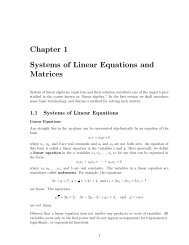
5.1 <strong>Functions</strong> of Two or More Variables<br />
Notation and Terminology<br />
The terminology and notation for functions of two or more variables is similar to that for<br />
functions of one variable. For example, the expression<br />
z = f(x,y)<br />
means that z is a function of x and y in the sense that a unique value of the dependent<br />
variable z is determined by specifying values for the independent variables x and y. Similarly,<br />
w = f(x,y,z)<br />
expresses w as a function x, y, and z, and<br />
u = f(x 1 ,x 2 ,...,x n )<br />
expresses u as a function of x 1 ,x 2 ,...,x n .<br />
As with functions of one variable, the independent variables of a function of two or more<br />
variables may be restricted to lie in some set D, which we call the domain of f. Sometimes<br />
the domain will be determined by physical restrictions on the variables. If the function is<br />
defined by a formula and if there are no physical restrictions or other restrictions stated<br />
explicitly, then it is understand that the domain consists of all points for which the formula<br />
yields a real value for the dependent variable. We call this the natural domain of the<br />
function.<br />
Definition 5.1 A function f of two variables, x and y, is a rule that assigns a unique<br />
real number f(x,y) to each point (x,y) in some set D in the xy-plane.<br />
Definition 5.2 A function f of three variables, x, y, and z, is a rule that assigns<br />
a unique real number f(x,y,z) to each point (x,y,z) in some set D in three dimensional<br />
space.<br />
79
MA112 Section 750001: Prepared by Dr.Archara Pacheenburawana 80<br />
Example 5.1 Let<br />
f(x,y) = 3x 2√ y −1<br />
Find f(1,4), f(0,9), f(t 2 ,t), f(ab,9b), and the natural domain of f.<br />
Solution .........<br />
Example 5.2 Sketch the natural domain of the function (a) f(x,y) = ln(x 2 −y) and (b)<br />
g(x,y) = 2x<br />
y −x 2.<br />
Solution .........<br />
Example 5.3 Let<br />
f(x,y,z) = √ 1−x 2 −y 2 −z 2<br />
Find f ( 0, 1 2 ,−1 2)<br />
and the natural domain of f.<br />
Solution .........<br />
Graphs of <strong>Functions</strong> of Two Variables<br />
Recall that for a function f of one variable, the graph of f(x) in the xy-plane was defined<br />
to be the graph of the equation y = f(x). Similarly, if f is a function of two variables, we<br />
define the graph of f(x,y) in xyz-space to be the graph of the equation z = f(x,y). In<br />
general, such a graph will be a surface in 3-space.<br />
Example 5.4 In each part, describe the graph of the function in an xyz-coordinate system.<br />
(a) f(x,y) = 1−x− 1 2 y (b) f(x,y) = √ 1−x 2 −y 2<br />
(c) f(x,y) = − √ x 2 +y 2<br />
Solution .........<br />
5.2 Limits and Continuity<br />
For a function of one variable there are two one-sided limits at a points x 0 , namely,<br />
lim f(x) and lim f(x)<br />
x→x + 0 x→x − 0<br />
reflecting the fact that there are only two directions fromwhich x can approach x 0 , the right<br />
or the left. For function of two or three variables the situation is more complicated because<br />
there are infinitely many different curves along which one point can approach another. Our<br />
first objective is to define the limit of f(x,y) as (x,y) approaches a point (x 0 ,y 0 ) along the<br />
curve C (and similarly for functions of three variables).<br />
If C is a smooth parametric curve in 2-space or 3-space that is represented by the<br />
equations<br />
x = x(t), y = y(t) or x = x(t), y = y(t), z = z(t)
MA112 Section 750001: Prepared by Dr.Archara Pacheenburawana 81<br />
and if x 0 = x(t 0 ),y 0 = y(t 0 ), and z 0 = z(t 0 ), then the limits<br />
lim<br />
(x,y) → (x 0 ,y 0 )<br />
(along C)<br />
f(x,y) and<br />
lim<br />
(x,y,z) → (x 0 ,y 0 ,z 0 )<br />
(along C)<br />
f(x,y,z)<br />
are defined by<br />
lim<br />
(x,y) → (x 0 ,y 0 )<br />
(along C)<br />
f(x,y) = lim<br />
t→t0<br />
f(x(t),y(t)) (5.1)<br />
lim<br />
(x,y,z) → (x 0 ,y 0 ,z 0 )<br />
(along C)<br />
f(x,y,z) = lim<br />
t→t0<br />
f(x(t),y(t),z(t)) (5.2)<br />
Example 5.5 Find the limit of the function<br />
as (x,y) → (0,0) along<br />
f(x,y) = − xy<br />
x 2 +y 2<br />
(a) the x-axis (b) the y-axis (c) the line y = x<br />
(d) the line y = −x (e) the parabola y = x 2<br />
Solution .........<br />
Relationships between General Limits and Limit Along Smooth<br />
Curve<br />
Theorem 5.1<br />
(a) If f(x,y) → L as (x,y) → (x 0 ,y 0 ), then f(x,y) → L as (x,y) → (x 0 ,y 0 ) along any<br />
smooth curve.<br />
(b) If the limit of f(x,y) fail to exit as (x,y) → (x 0 ,y 0 ) along some smooth curve, or if<br />
f(x,y) has different limit as (x,y) → (x 0 ,y 0 ) along two different smooth curves, then<br />
the limit of f(x,y) does not exist as (x,y) → (x 0 ,y 0 ).<br />
Example 5.6 The limit<br />
lim − xy<br />
(x,y)→(0,0) x 2 +y 2<br />
does not exist because in Example 5.5 we found two different smooth curves along which this<br />
limit had different values. Specifically,<br />
lim<br />
(x,y) → (0,0)<br />
(along y = 0)<br />
− xy<br />
x 2 +y 2 = 0 and<br />
lim<br />
(x,y) → (0,0)<br />
(along y = x)<br />
− xy<br />
x 2 +y 2 = −1 2 .<br />
✠
MA112 Section 750001: Prepared by Dr.Archara Pacheenburawana 82<br />
Continuity<br />
Definition 5.3 A function f(x,y) is said to be continuous at (x 0 ,y 0 ) if f(x 0 ,y 0 ) is<br />
defined and if<br />
lim<br />
(x,y)→(x 0 ,y 0 ) f(x,y) = f(x 0,y 0 )<br />
In addition, if f is continuous at every point in an open set D, then we say that f is<br />
continuous on D, and if f is continuous at every point in the xy-plane, then we say that<br />
f is continuous everywhere.<br />
Theorem 5.2<br />
(a) If g(x) is continuous at x 0 and h(y) is continuous at y 0 , then f(x,y) = g(x)h(y) is<br />
continuous at (x 0 ,y 0 ).<br />
(b) If h(x,y) is continuous at (x 0 ,y 0 ) and g(u) is continuous at u = h(x 0 ,y 0 ), then the<br />
composition f(x,y) = g(h(x,y)) is continuous at (x 0 ,y 0 ).<br />
(c) If f(x,y) is continuous at (x 0 ,y 0 ) and if x(t) and y(t) is continuous at t 0 with x(t 0 ) =<br />
x 0 and y(t 0 ) = y 0 , then the composition f(x(t),y(t)) is continuous at t 0 .<br />
Example 5.7 Show that the functions f(x,y) = 3x 2 y 5 and f(x,y) = sin(3x 2 y 5 ) are continuous<br />
everywhere.<br />
Solution .........<br />
Recognizing continuous <strong>Functions</strong><br />
• A composition of continuous functions is continuous.<br />
• A sum, difference, or product of continuous functions is continuous.<br />
• A quotient of continuous functions is continuous, except where the denominator is<br />
zero.<br />
Example 5.8 Evaluate<br />
Solution .........<br />
lim<br />
(x,y)→(−1,2)<br />
Example 5.9 Since the function<br />
xy<br />
x 2 +y 2.<br />
f(x,y) = x3 y 2<br />
1−xy<br />
is a quotient of continuous functions, it is continuous except where 1−xy = 0. Thus f(x,y)<br />
is continuous everywhere except on the hyperbola xy = 1.<br />
✠
MA112 Section 750001: Prepared by Dr.Archara Pacheenburawana 83<br />
5.3 Partial Derivatives<br />
Partial Derivatives of <strong>Functions</strong> of Two Variables<br />
If z = f(x,y), then one can inquire how the value of z changes if y is held fixed and x is<br />
allowed to vary, or if x is held fixed and y is allowed to vary. For example, the ideal gas<br />
law in physics states that under appropriate conditions the pressure exerted by a gas is a<br />
function of the volume of the gas and its temperature. Thus, a physicist studying gases<br />
might be interested in the rate of change of the pressure if the volume is held fixed and the<br />
temperature is allowed to vary, or if the temperature is held fixed and the volume is allowed<br />
to vary. We now define a derivative that describes such rates of change.<br />
Definition 5.4 If z = f(x,y) and (x 0 ,y 0 ) is a point in the domain of f, then the partial<br />
derivative of f with respect to x at (x 0 ,y 0 ) [ also called the partial derivative of<br />
z with respect to x at (x 0 ,y 0 ) ] is the derivative at x 0 of the function that results when<br />
y = y 0 is held fixed and x is allowed to vary. This partial derivative is denoted by f x (x 0 ,y 0 )<br />
and is given by<br />
f x (x 0 ,y 0 ) = d<br />
dx [f(x,y 0)] ∣ = lim<br />
x=x0<br />
∆x→0<br />
f(x 0 +∆x,y 0 )−f(x 0 ,y 0 )<br />
∆x<br />
(5.3)<br />
Similarly, the partial derivative of f with respect to y at (x 0 ,y 0 ) [ also called the<br />
partial derivative of z with respect to y at (x 0 ,y 0 ) ] is the derivative at y 0 of the<br />
function that results when x = x 0 is held fixed and y is allowed to vary. This partial<br />
derivative is denoted by f y (x 0 ,y 0 ) and is given by<br />
f y (x 0 ,y 0 ) = d<br />
dy [f(x 0,y)] ∣ = lim<br />
y=y0<br />
∆y→0<br />
f(x 0 ,y 0 +∆y)−f(x 0 ,y 0 )<br />
∆y<br />
Example 5.10 Find f x (1,0) and f y (2,−1) for the function f(x,y) = 3x 2 +x 3 y +4y 2 .<br />
Solution .........<br />
The Partial Derivative <strong>Functions</strong><br />
(5.4)<br />
Formulas (5.3) and (5.4) define the partial derivatives of a function at a specific point<br />
(x 0 ,y 0 ). However, often it will be desirable to omit the subscripts and think of the partial<br />
derivatives as a functions of the variables x and y. These functions are<br />
and<br />
f(x+∆x,y)−f(x,y)<br />
f x (x,y) = lim<br />
∆x→0 ∆x<br />
f(x,y +∆y)−f(x,y)<br />
f y (x,y) = lim<br />
∆y→0 ∆y<br />
The following example gives an alternative way of performing the computations in Example<br />
5.10.
MA112 Section 750001: Prepared by Dr.Archara Pacheenburawana 84<br />
Example 5.11 Find f x (x,y) and f y (x,y) for f(x,y) = 3x 2 + x 3 y + 4y 2 , and use those<br />
partial derivatives to compute f x (1,0) and f y (2,−1).<br />
Solution .........<br />
Partial Derivative Notation<br />
If z = f(x,y), then the partial derivatives f x and f y are also denoted by the symbols<br />
∂f<br />
∂x , ∂z<br />
∂x<br />
and<br />
∂f<br />
∂y , ∂z<br />
∂y<br />
Some typical notations for the partial derivatives of z = f(x,y) at a point (x 0 ,y 0 ) are<br />
∂f<br />
∂z<br />
∂x∣ ,<br />
∂f<br />
∂f<br />
x=x0 ,y=y 0<br />
∂x∣ (x0 ,y 0 ),<br />
∂x∣ (x0 ,y 0 ),<br />
∂x (x ∂z<br />
0,y 0 ),<br />
∂x (x 0,y 0 )<br />
Example 5.12 Find ∂z<br />
∂x<br />
Solution .........<br />
and<br />
∂z<br />
∂y if z = exy + x y .<br />
Partial Derivatives Viewed as Rates of Change and Slopes<br />
Recall that if y = f(x), then the value of f ′ (x 0 ) can be interpreted either as the rate of<br />
change of y with respect to x at x 0 or as the slope of the tangent line to the graph of f at<br />
x 0 . Partial derivatives have analogous interpretations.<br />
Suppose that C 1 is the intersection of the surface z = f(x,y) with the plane y = y 0 and<br />
that C 2 is its intersection with the plane x = x 0 . Thus, f x (x,y 0 ) can be interpreted as the<br />
rate of change of z with respect to x along the curve C 1 , and f y (x 0 ,y) can be interpreted as<br />
the rate of change of z with respect to y along the curve C 2 . In particular, f x (x 0 ,y 0 ) is the<br />
rate of change of z with respect to x along the curve C 1 at the point (x 0 ,y 0 ), and f y (x 0 ,y 0 )<br />
is the rate of change of z with respect to y along the curve C 2 at the point (x 0 ,y 0 ).<br />
Example 5.13 For a real gas, van der Waals’s equation states that<br />
( )<br />
P + n2 a<br />
(V −nb) = nRT<br />
V 2<br />
Here, P is the pressure of the gas, V is the volume of the gas, T is the temperature (in<br />
degrees Kelvin), n is the number of moles of gas, R is the universal gas constant and a and<br />
b are constants. Compute and interpret P V and T P<br />
Solution .........<br />
Geometrically, f x (x 0 ,y 0 ) can be viewed as the slope of the tangent line to the curve C 1<br />
at the point (x 0 ,y 0 ), and f y (x 0 ,y 0 ) can be viewed as the slope of the tangent line to the<br />
curve C 2 at the point (x 0 ,y 0 ). We will call f x (x 0 ,y 0 ) the slope of the surface in the<br />
x-direction at (x 0 ,y 0 ) and f y (x 0 ,y 0 ) the slope of the surface in the y-direction at<br />
(x 0 ,y 0 ).
MA112 Section 750001: Prepared by Dr.Archara Pacheenburawana 85<br />
Example 5.14 Let f(x,y) = x 2 y +5y 3 .<br />
(a) Find the slope of the surface z = f(x,y) in the x-direction at the point (1,−2).<br />
(b) Find the slope of the surface z = f(x,y) in the y-direction at the point (1,−2).<br />
Solution .........<br />
Implicit Partial Differentiation<br />
(<br />
Example 5.15 Find the slope of the sphere x 2 +y 2 +z 2 = 1 in the y-direction at the points<br />
2 , 1, ) ( 2<br />
3 3 3 and 2 , ) 1<br />
3 3 ,−2 3 .<br />
Solution .........<br />
Example 5.16 Suppose that D = √ x 2 +y 2 is the length of the diagonal of a rectangle<br />
whose sides have lengths x and y that are allowed to vary. Find the formula for the rate of<br />
change of D with respect to x if x varies with y held constant, and use this formula to find<br />
the rate of change of D with respect to x at the point where x = 3 and y = 4.<br />
Solution .........<br />
Partial Derivatives of <strong>Functions</strong> with More Than Two Variables<br />
For a function f(x,y,z) of three variables, there are three partial derivatives:<br />
f x (x,y,z), f y (x,y,z), f z (x,y,z)<br />
The partial derivative f x is calculated by holding y and z constant and differentiating with<br />
respect to x. For f y the variables x and z are held constant, and for f z the variables x and<br />
y are held constant. If a dependent variable<br />
w = f(x,y,z)<br />
is used, then the three partial derivatives of f can be denoted by<br />
∂w<br />
∂x , ∂w ∂w<br />
, and<br />
∂y ∂z<br />
Example 5.17 If f(x,y,z) = x 3 y 2 z 4 +2xy +z, then<br />
f x (x,y,z) =<br />
f y (x,y,z) =<br />
f z (x,y,z) =<br />
f z (−1,1,2) =
MA112 Section 750001: Prepared by Dr.Archara Pacheenburawana 86<br />
Example 5.18 If f(ρ,θ,φ) = ρ 2 cosφsinθ, then<br />
f ρ (ρ,θ,φ) =<br />
f θ (ρ,θ,φ) =<br />
f φ (ρ,θ,φ) =<br />
In general, if f(v 1 ,v 2 ,...,v n ) is a function of n variables, there are n partial derivatives<br />
of f, each of which is obtained by holding n −1 of the variables fixed and differentiating<br />
the function f with respect to the remaining variable. If w = f(v 1 ,v 2 ,...,v n ), then these<br />
partial derivatives are denoted by<br />
∂w<br />
∂v 1<br />
,<br />
∂w<br />
,..., ∂w<br />
∂v 2 ∂v n<br />
where ∂w/∂v i is obtained by holding all variables except v i fixed and differentiating with<br />
respect to v i .<br />
Example 5.19 Find<br />
for i = 1,2,...,n.<br />
[√ ]<br />
∂<br />
x 2 1 +x 2 2 +···+x<br />
∂x 2 n<br />
i<br />
Solution .........<br />
Higher-Order Partial Derivatives<br />
Suppose that f is a function of two variables x and y. Since the partial derivatives ∂f/∂x<br />
and ∂f/∂y are also functions of x and y, these functions may themselves have partial<br />
derivatives. This gives rise to four possible second-order partial derivatives of f, which are<br />
defined by<br />
∂ 2 f<br />
∂x = ∂ ( ) ∂f ∂ 2 f<br />
= f 2 xx<br />
∂x ∂x ∂y = ∂ ( ) ∂f<br />
= f 2 yy<br />
∂y ∂y<br />
Differentiate twice<br />
with respect to x.<br />
∂ 2 f<br />
∂y∂x = ∂ ( ) ∂f<br />
∂y ∂x<br />
Differentiate first with<br />
respect to x and then<br />
with respect to y.<br />
= f xy<br />
∂ 2 f<br />
∂x∂y = ∂<br />
∂x<br />
Differentiate twice<br />
with respect to y.<br />
( ) ∂f<br />
= f yx<br />
∂y<br />
Differentiate first with<br />
respect to y and then<br />
with respect to x.<br />
The last two cases are called the mixed second-order partial derivatives or the mixed<br />
second partials. Also, the derivatives ∂f/∂x and ∂f/∂x are often called the first-order<br />
partial derivatives when it is necessary to distinguish them from higher-order partial<br />
derivatives.
MA112 Section 750001: Prepared by Dr.Archara Pacheenburawana 87<br />
Example 5.20 Find the second-order partial derivatives of f(x,y) = x 2 y −y 3 +lnx.<br />
Solution .........<br />
Third-order, fourth-order, and higher-order partial derivatives can be obtained by successive<br />
differentiation. Some possibilities are<br />
∂ 3 f<br />
∂x = ∂ ( ) ∂ 2 f<br />
∂ 4 f<br />
= f 3 ∂x ∂x 2 xxx<br />
∂y = ∂ ( ) ∂ 3 f<br />
= f 4 ∂y ∂y 3 yyyy<br />
∂ 3 f<br />
∂y 2 ∂x = ∂ ( ) ∂ 2 f ∂ 4 f<br />
= f xyy<br />
∂y ∂y∂x ∂y 2 ∂x = ∂ ( ) ∂ 3 f<br />
= f 2 ∂y ∂y∂x 2 xxyy<br />
Example 5.21 Let f(x,y) = cos(xy)−x 3 +y 4 . Find f xyy .<br />
Solution .........<br />
Equality of Mixed Partials<br />
Theorem 5.3 Let f be a function of two variables. If f xy and f yx are continuous on some<br />
open disk, then f xy = f yx on that disk.<br />
5.4 Differentiability, Differentials, and Local Linearity<br />
Differentiability<br />
Definition 5.5 A function f of two variables is said to be differentiable at (x 0 ,y 0 ) provided<br />
f x (x 0 ,y 0 ) and f y (x 0 ,y 0 ) both exist and<br />
∆f −f x (x 0 ,y 0 )∆x−f y (x 0 ,y 0 )∆y<br />
lim √ = 0 (5.5)<br />
(∆x,∆y)→(0,0) (∆x)2 +(∆y) 2<br />
NoteForafunctionf(x,y),thesymbol ∆f, calledtheincrement off, denotes thechange<br />
in the value of f(x,y) that results when (x,y) varies from some initial position (x 0 ,y 0 ) to<br />
some new position (x 0 +∆x,y 0 +∆y); thus<br />
∆f = f(x 0 +∆x,y 0 +∆y)−f(x 0 ,y 0 )<br />
Example 5.22 Use Definition 5.5 to prove that f(x,y) = x 2 +y 2 is differentiable at (0,0).<br />
Solution .........<br />
Definition 5.6 A function f of three variables is said to be differentiable at (x 0 ,y 0 ,z 0 )<br />
provided f x (x 0 ,y 0 ,z 0 ), f y (x 0 ,y 0 ,z 0 ), and f z (x 0 ,y 0 ,z 0 ) exist and<br />
∆f −f x (x 0 ,y 0 ,z 0 )∆x−f y (x 0 ,y 0 ,z 0 )∆y −f z (x 0 ,y 0 ,z 0 )∆z<br />
lim √ = 0 (5.6)<br />
(∆x,∆y,∆z)→(0,0) (∆x)2 +(∆y) 2 +(∆z) 2<br />
If a function f of two variables is differentiable at each point of the region R in the<br />
xy-plane, then we say that f is differentiable on R; and if f is differentiable at every<br />
point in the xy-plane, then we say that f is differentiable everywhere. For a function<br />
f of three variables we have corresponding conventions.
MA112 Section 750001: Prepared by Dr.Archara Pacheenburawana 88<br />
Differentiability and Continuity<br />
Theorem 5.4 If a function is differentiable at a point, then it is continuous at that point.<br />
Theorem 5.5 If all first-order partial derivatives of f exist and are continuous at a point,<br />
then f is differentiable at that point.<br />
For example, consider the function<br />
f(x,y,z) = x+yz<br />
Since f x (x,y,z) = 1,f y (x,y,z) = z, and f z (x,y,z) = y are defined and continuous everywhere,<br />
we conclude that f is differentiable everywhere.<br />
Differentials<br />
If z = f(x,y) is differentiable at a point (x 0 ,y 0 ), we let<br />
dz = f x (x 0 ,y 0 )dx+f y (x 0 ,y 0 )dy (5.7)<br />
denote a new function with dependent variable dz and independent variables dx and dy.<br />
We refer to this function (also denoted df) as the total differential of z at (x 0 ,y 0 ) or as<br />
the total differential of f at (x 0 ,y 0 ). Similarly, for a function w = f(x,y,z) of three<br />
variables we have the total differential of w at (x 0 ,y 0 ,z 0 ),<br />
dw = f x (x 0 ,y 0 ,z 0 )dx+f y (x 0 ,y 0 ,z 0 )dy +f z (x 0 ,y 0 ,z 0 )dz (5.8)<br />
which is also referred toas the total differential of f at (x 0 ,y 0 ,z 0 ). It is common practice<br />
to omit the subscripts and write Equations (5.7) and (5.8) as<br />
and<br />
dz = f x (x,y)dx+f y (x,y)dy (5.9)<br />
dw = f x (x,y,z)dx+f y (x,y,z)dy+f z (x,y,z)dz (5.10)<br />
In the two-variable case, the approximation<br />
can be written in the form<br />
∆f ≈ f x (x 0 ,y 0 )∆x+f y (x 0 ,y 0 )∆y<br />
∆f ≈ df (5.11)<br />
for dx = ∆x and dy = ∆y. Equivalently, we can write approximation (5.11) as<br />
∆z ≈ dz (5.12)<br />
Example 5.23 Use a total differential to approximate the change in z = xy 2 from it value<br />
at (0.5,1.0) to its value at (0.503,1.004). Compare this estimate with the actual change in<br />
z.<br />
Solution .........
MA112 Section 750001: Prepared by Dr.Archara Pacheenburawana 89<br />
Local Linear Approximations<br />
When f(x,y) is differentiable at (x 0 ,y 0 ) we get<br />
L(x,y) = f(x 0 ,y 0 )+f x (x 0 ,y 0 )(x−x 0 )+f y (x 0 ,y 0 )(y −y 0 )<br />
and refer to L(x,y) as the local linear approximation to f at (x 0 ,y 0 ).<br />
Example 5.24 Let L(x,y) denote the local linear approximation to f(x,y) = √ x 2 +y 2 at<br />
the point (3,4). Compare the error in approximating<br />
f(3.04,3.98) = √ (3.04) 2 +(3.98) 2<br />
by L(3.04,3.98) with the distance between the points (3,4) and (3.04,3.98).<br />
Solution .........<br />
is<br />
Forafunctionf(x,y,z)thatisdifferentiableat(x 0 ,y 0 ,z 0 ),thelocallinearapproximation<br />
L(x,y,z) = f(x 0 ,y 0 ,z 0 )+f x (x 0 ,y 0 ,z 0 )(x−x 0 )<br />
+f y (x 0 ,y 0 ,z 0 )(y −y 0 )+f z (x 0 ,y 0 ,z 0 )(z −z 0 )<br />
5.5 The Chain Rule<br />
The Chain Rule for Derivatives<br />
Theorem 5.6 (Chain Rule for Derivatives) If x = x(t) and y = y(t) are differentiable<br />
at t, and if z = f(x,y) is differentiable at the point (x,y) = (x(t),y(t)), then<br />
z = f(x(t),y(t)) is differentiable at t and<br />
dz<br />
dt = ∂z dx<br />
∂x dt + ∂z dy<br />
∂y dt<br />
(5.13)<br />
where the ordinary derivatives are evaluated at t and the partial derivatives are evaluated<br />
at (x,y).<br />
If each of the functions x = x(t), y = y(t), and z = z(t) is differentiable at t, and if w =<br />
f(x,y,z) is differentiable at the point (x,y,z) = (x(t),y(t),z(t)), then w = f(x(t),y(t),z(t))<br />
is differentiable at t and<br />
dw<br />
dt = ∂w dx<br />
∂x dt + ∂w dy<br />
∂y dt + ∂w dz<br />
(5.14)<br />
∂z dt<br />
where the ordinary derivatives are evaluated at t and the partial derivatives are evaluated<br />
at (x,y,z).<br />
Formula (5.13) can be represented schematically by a “tree diagram” that is constructed<br />
as follows.
MA112 Section 750001: Prepared by Dr.Archara Pacheenburawana 90<br />
z<br />
∂z<br />
∂x<br />
∂z<br />
∂y<br />
x<br />
dx<br />
dt<br />
y<br />
dy<br />
dt<br />
t<br />
dz<br />
dt = ∂z dx<br />
∂x dt + ∂z dy<br />
∂y dt<br />
t<br />
Example 5.25 Suppose that<br />
Use the chain rule to find dz/dt.<br />
Solution .........<br />
Example 5.26 Suppose that<br />
z = x 2 e y , x(t) = t 2 −1, y(t) = sint<br />
z = √ xy +y, x = cosθ, y = sinθ<br />
Use the chain rule to find dz/dθ when θ = π/2.<br />
Solution .........<br />
Example 5.27 Suppose that<br />
w = √ x 2 +y 2 +z 2 , x = cosθ, y = sinθ, z = tanθ<br />
Use the chain rule to find dw/dθ.<br />
Solution .........<br />
The Chain Rule for Partial Derivatives<br />
Theorem 5.7 (Chain Rule for Partial Derivatives) If x = x(u,v) and y = y(u,v)<br />
have first-order derivatives at the point (u,v), and if z = f(x,y) is differentiable at the point<br />
(x,y) = (x(u,v),y(u,v)), then z = f(x(u,v),y(u,v)) has first-order partial derivatives at<br />
the point (u,v) given by<br />
∂z<br />
∂u = ∂z ∂x<br />
∂x∂u + ∂z ∂y<br />
∂y∂u<br />
and<br />
∂z<br />
∂v = ∂z ∂x<br />
∂x∂v + ∂z ∂y<br />
∂y∂v<br />
If each function x = x(u,v), y = y(u,v), and z = z(u,v) have first-order derivatives at<br />
the point (u,v), and if the function w = f(x,y,z) is differentiable at the point (x,y,z) =
MA112 Section 750001: Prepared by Dr.Archara Pacheenburawana 91<br />
(x(u,v),y(u,v),z(u,v)), then the function w = f(x(u,v),y(u,v),z(u,v)) has first-order<br />
partial derivatives at the point (u,v) given by<br />
∂w<br />
∂u = ∂w ∂x<br />
∂x ∂u + ∂w ∂y<br />
∂y ∂u + ∂w ∂z<br />
∂z ∂u<br />
and<br />
∂w<br />
∂v = ∂w ∂x<br />
∂x ∂v + ∂w ∂y<br />
∂y ∂v + ∂w ∂z<br />
∂z ∂v<br />
The following figure shows tree diagrams for the formulas in Theorem 5.7.<br />
z<br />
z<br />
∂z<br />
∂x<br />
∂z<br />
∂y<br />
∂z<br />
∂x<br />
∂z<br />
∂y<br />
x<br />
y<br />
x<br />
y<br />
∂x<br />
∂u<br />
∂x<br />
∂v<br />
∂y<br />
∂u<br />
∂y<br />
∂v<br />
∂x<br />
∂u<br />
∂x<br />
∂v<br />
∂y<br />
∂u<br />
∂y<br />
∂v<br />
u v u v<br />
∂z<br />
∂u = ∂z ∂x<br />
∂x∂u + ∂z ∂y<br />
∂y∂u<br />
u v u v<br />
∂z<br />
∂v = ∂z ∂x<br />
∂x∂v + ∂z ∂y<br />
∂y∂v<br />
w<br />
∂w<br />
∂x<br />
∂w<br />
∂y<br />
∂w<br />
∂z<br />
x y z<br />
∂x<br />
∂u<br />
∂x<br />
∂v<br />
∂y<br />
∂u<br />
∂y<br />
∂v<br />
∂z<br />
∂u<br />
∂z<br />
∂v<br />
u v u v u v<br />
∂w<br />
∂u = ∂w ∂x<br />
∂x ∂u + ∂w ∂y<br />
∂y ∂u + ∂w ∂z<br />
∂z ∂u<br />
∂w<br />
∂v = ∂w ∂x<br />
∂x ∂v + ∂w ∂y<br />
∂y ∂v + ∂w ∂z<br />
∂z ∂v<br />
Example 5.28 Given that<br />
z = e xy , x(u,v) = 3usinv, y(u,v) = 4v 2 u<br />
find ∂z/∂u and ∂z/∂v using the chain rule.<br />
Solution .........
MA112 Section 750001: Prepared by Dr.Archara Pacheenburawana 92<br />
Example 5.29 Suppose that<br />
w = e xyz , x = 3u+v, y = 3u−v, z = u 2 v<br />
Use appropriate forms of the chain rule to find ∂w/∂u and ∂w/∂v.<br />
Solution .........<br />
Other Versions of the Chain Rule<br />
Although we will not prove it, the chain rule extends to functions w = f(v 1 ,v 2 ,...,v n ) of<br />
n variables. For example, if each v i is a function of t, i = 1,2,...,n, the relevant formula is<br />
dw<br />
dt = ∂w dv 1<br />
∂v 1 dt + ∂w dv 2 ∂w dv n<br />
+···+<br />
∂v 2 dt ∂v n dt<br />
(5.15)<br />
There are infinitely many variations of the chain rule, depending on the number of<br />
variablesandthechoice ofindependent anddependent variables. Agoodworking procedure<br />
is to use tree diagrams to derive new versions of the chain rule as needed.<br />
Example 5.30 Suppose that w = x 2 +y 2 +z 2 and<br />
x = ρsinφcosθ, y = ρsinφsinθ, z = ρcosφ<br />
Use appropriate forms of the chain rule to find ∂w/∂ρ and ∂w/∂θ.<br />
Solution .........<br />
Example 5.31 Suppose that<br />
w = xy +yz, y = sinx, z = e x<br />
Use appropriate form of the chain rule to find dw/dx.<br />
Solution .........<br />
Implicit Differentiation<br />
Consider the special case where z = f(x,y) is a function of x and y and y is a differentiable<br />
function of x. Equation (5.13) then becomes<br />
dz<br />
dx = ∂f dx<br />
∂xdx + ∂f dy<br />
∂y dx = ∂f<br />
∂x + ∂f dy<br />
∂y dx<br />
(5.16)<br />
This result can be used to find derivatives of functions that are defined implicitly. For<br />
example, suppose that the equation<br />
f(x,y) = c (5.17)
MA112 Section 750001: Prepared by Dr.Archara Pacheenburawana 93<br />
defines y implicitly as a differentiable function of x and we are interested in finding dy/dx.<br />
Differentiating both sides of (5.17) with respect to x and applying (5.16) yields<br />
Thus, if ∂f/∂y ≠ 0, we obtain<br />
In summary, we have the following result.<br />
∂f<br />
∂x + ∂f dy<br />
∂y dx = 0<br />
dy<br />
dx = −∂f/∂x ∂f/∂y<br />
Theorem 5.8 If the equation f(x,y) = c defines y implicitly as a differentiable function<br />
of x, and if ∂f/∂y ≠ 0, then<br />
dy<br />
dx = −∂f/∂x<br />
(5.18)<br />
∂f/∂y<br />
Example 5.32 Given that<br />
x 3 +y 2 x−3 = 0<br />
find dy/dx using (5.18), and check the result using implicit differentiation.<br />
Solution .........<br />
Theorem 5.9 If the equation f(x,y,z) = c defines z implicitly as a differentiable function<br />
of x and y, and if ∂f/∂z ≠ 0, then<br />
dz<br />
dx = −∂f/∂x ∂f/∂z<br />
and<br />
dz<br />
dy = −∂f/∂y ∂f/∂z<br />
Example<br />
(<br />
5.33 Consider the sphere x 2 +y 2 +z 2 = 1. Find ∂z/∂x and ∂z/∂y at the point<br />
2 , 1 , ) 2<br />
3 3 3 .<br />
Solution .........<br />
5.6 Directional Derivatives and Gradients<br />
Directional Derivatives<br />
Definition 5.7 If f(x,y) is a function of x and y, and if u = u 1 i + u 2 j is a unit vector,<br />
then the directional derivative of f in the direction of u at (x 0 ,y 0 ) is denoted by<br />
D u f(x 0 ,y 0 ) and is defined by<br />
D u f(x 0 ,y 0 ) = d ds [f(x 0 +su 1 ,y 0 +su 2 )] s=0 (5.19)<br />
provided this derivative exists.
MA112 Section 750001: Prepared by Dr.Archara Pacheenburawana 94<br />
Geometrically, D u f(x 0 ,y 0 ) can be interpreted as the slope of the surface z = f(x,y)<br />
in the direction of u at the point (x 0 ,y 0 ,f(x 0 ,y 0 )). Usually the value of D u f(x 0 ,y 0 ) will<br />
depend on both the point (x 0 ,y 0 ) and the direction u. Thus, at a fixed point the slope of<br />
the surface may vary with the direction.<br />
Example 5.34 Let f(x,y) = xy. Find and interpret D u f(1,2) for the unit vector u =<br />
√<br />
3<br />
2 i+ 1 2 j.<br />
Solution .........<br />
The definition of a directional derivative for a function f(x,y,z) of three variables is<br />
similar to Definition 5.7.<br />
Definition 5.8 If u = u 1 i+u 2 j+u 3 k is a unit vector, and if f(x,y,z) is a function of x,<br />
y, and z, then the directional derivative of f in the direction of u at (x 0 ,y 0 ,z 0 ) is<br />
denoted by D u f(x 0 ,y 0 ,z 0 ) and is defined by<br />
provided this derivative exists.<br />
D u f(x 0 ,y 0 ,z 0 ) = d ds [f(x 0 +su 1 ,y 0 +su 2 ,z 0 +su 3 )] s=0 (5.20)<br />
For a function that is differentiable at a point, directional derivatives exist in every<br />
direction from the point and can be computed directly in terms of the first-order partial<br />
derivatives of the function.<br />
Theorem 5.10<br />
(a) If f(x,y) is differentiable at (x 0 ,y 0 ) and if u = u 1 i + u 2 j is a unit vector, then the<br />
directional derivative D u f(x 0 ,y 0 ) exists and is given by<br />
D u f(x 0 ,y 0 ) = f x (x 0 ,y 0 )u 1 +f y (x 0 ,y 0 )u 2 (5.21)<br />
(b) If f(x,y,z) is differentiable at (x 0 ,y 0 ,z 0 ) and if u = u 1 i+u 2 j+u 3 k is a unit vector,<br />
then the directional derivative D u f(x 0 ,y 0 ,z 0 ) exists and is given by<br />
D u f(x 0 ,y 0 ,z 0 ) = f x (x 0 ,y 0 ,x 0 )u 1 +f y (x 0 ,y 0 ,z 0 )u 2 +f z (x 0 ,y 0 ,z 0 )u 3 (5.22)<br />
Example 5.35 For f(x,y) = x 2 y−4y 3 , compute D u f(2,1) where u is a unit vector in the<br />
direction from (2,1) to (4,0).<br />
Solution .........<br />
Recall that a unit vector u in the xy-plane can be expressed as<br />
u = cosφi+sinφj<br />
where φ is the angle from the positive x-axis to u. Thus, Formula (5.21) can also be<br />
expressed as<br />
D u f(x 0 ,y 0 ) = f x (x 0 ,y 0 )cosφ+f y (x 0 ,y 0 )sinφ (5.23)
MA112 Section 750001: Prepared by Dr.Archara Pacheenburawana 95<br />
Example 5.36 Find the directional derivative of f(x,y) = e xy at (−2,0) in the direction<br />
of the unit vector that makes an angle of π/3 with the positive x-axis.<br />
Solution .........<br />
Example 5.37 Find the directional derivative of f(x,y,z) = x 2 y−yz 3 +z at (1,−2,0) in<br />
the direction of the vector a = 2i+j−2k.<br />
Solution .........<br />
The Gradient<br />
Definition 5.9<br />
(a) If f is a function of x and y, then the gradient of f is defined by<br />
∇f(x,y) = f x (x,y)i+f y (x,y)j (5.24)<br />
(b) If f is a function of x, y, and z, then the gradient of f is defined by<br />
∇f(x,y,z) = f x (x,y,z)i+f y (x,y,z)j+f k (x,y,z)k (5.25)<br />
Formulas (5.21) and (5.22) can now be written as<br />
D u f(x 0 ,y 0 ) = ∇f(x 0 ,y 0 )·u (5.26)<br />
and<br />
D u f(x 0 ,y 0 ,z 0 ) = ∇f(x 0 ,y 0 ,z 0 )·u (5.27)<br />
respectively. For example, using Formula (5.27) our solution to Example 5.37 would take<br />
the form<br />
D u f(1,−2,0) = ∇f(1,−2,0)·u<br />
( 2<br />
= (−4i+j+k)·<br />
3 i+ 1 3 j− 2 )<br />
3 k ( 2<br />
= (−4) +<br />
3)<br />
1 3 − 2 3 = −3<br />
Formula (5.26) can be interpreted to mean that the slope of the surface z = f(x,y) at the<br />
point (x 0 ,y 0 ) in the direction of u is the dot product of the gradient with u.
MA112 Section 750001: Prepared by Dr.Archara Pacheenburawana 96<br />
Properties of the Gradient<br />
Theorem 5.11 Let f be a function of either two variables or three variables, and let P<br />
denote the point P(x 0 ,y 0 ) or P(x 0 ,y 0 ,z 0 ), respectively. Assume that f is differentiable at<br />
P.<br />
(a) If ∇f = 0 at P, then all directional derivatives of f at P are zero.<br />
(b) If ∇f ≠ 0 at P, then amongall possibledirectional derivativesof f at P, the derivative<br />
in the direction of ∇f at P has the largest value. The value of this largest directional<br />
derivative is ‖∇f‖ at P.<br />
(c) If ∇f ≠ 0 at P, then amongall possibledirectional derivativesof f at P, the derivative<br />
in the direction opposite to that of ∇f at P has the smallest value. The value of this<br />
smallest directional derivative is −‖∇f‖ at P.<br />
Example 5.38 Let f(x,y) = x 2 e y . Find the maximum value of a directional derivative at<br />
(−2,0), and find the unit vector in the direction in which the maximum value occurs.<br />
Solution .........
•<br />
•<br />
•<br />
•<br />
•<br />
•<br />
•<br />
•<br />
•<br />
•<br />
•<br />
•<br />
•<br />
•<br />
•<br />
•<br />
•<br />
•<br />
•<br />
•<br />
•<br />
•<br />
•<br />
•<br />
•<br />
•<br />
•<br />
•<br />
•<br />
•<br />
•<br />
•<br />
•<br />
•<br />
•<br />
•<br />
•<br />
•<br />
•<br />
•<br />
•<br />
•<br />
<strong>Chapter</strong> 6<br />
Multiple Integrals<br />
6.1 Double Integrals<br />
Volume<br />
Recall that the definite integral of a function of one variable<br />
∫ b<br />
n∑<br />
f(x)dx = lim f(x ∗ k )∆x k = lim<br />
max∆x k →0<br />
n→+∞<br />
a<br />
k=1<br />
n∑<br />
f(x ∗ k )∆x k (6.1)<br />
arose from the problem of finding areas under curves. Integrals of functions of two variables<br />
arise from the problem of finding volumes under surfaces.<br />
The Volume Problem. Given a function f of two variables that is continuous<br />
and nonnegative on a region R in the xy-plane, find the volume of the solid<br />
enclosed between the surface z = f(x,y) and the region R.<br />
The procedure for finding the volume V of the solid will be similar to the limiting process<br />
used for finding areas. We proceed as follows:<br />
• Using lines parallel to the coordinate axes, divide the rectangle enclosing the region R<br />
intosubrectangles, andexcludefromconsiderationallthosesubrectanglesthatcontain<br />
any points outside of R. This leaves only rectangles that are subset of R. Assume<br />
that there are n such rectangles, and denote the area of the kth such rectangle by<br />
∆A k .<br />
y<br />
k=1<br />
(x ∗ k ,y∗ k )<br />
Area ∆A k<br />
x<br />
97
MA112 Section 750001: Prepared by Dr.Archara Pacheenburawana 98<br />
• Choose any arbitrary point in each subrectangle, and denote the point in the kth<br />
subrectangle by (x ∗ k ,y∗ k ). The product f(x∗ k ,y∗ k )∆A k is the volume of a rectangular<br />
parallelepiped with base area ∆A k and height f(x ∗ k ,y∗ k ), so the sum<br />
n∑<br />
f(x ∗ k ,y∗ k )∆A k<br />
k=1<br />
can be view as an approximation to the volume V of the entire solid.<br />
• If we repeat the above process with more and more subdivisions in such a way that<br />
both the lengths and the widths of the subrectangles approach zero, then the exact<br />
volume of the solid will be<br />
V = lim<br />
n→+∞<br />
n∑<br />
f(x ∗ k,yk)∆A ∗ k<br />
k=1<br />
Definition 6.1 (Volume Under a Surface). If f is a function of two variables that is<br />
continuous and nonnegative on a region R in the xy-plane, then the volume of the solid<br />
enclosed between the surface z = f(x,y) and the region R is defined by<br />
V = lim<br />
n→+∞<br />
n∑<br />
f(x ∗ k ,y∗ k )∆A k (6.2)<br />
k=1<br />
Here, n → +∞ indicates the process of increasing the number of subrectangles of the rectangle<br />
enclosing R in such a way that both the lengths and the widths of the subrectangles<br />
approach zero.<br />
Definition of a Double Integral<br />
Thesumsin(6.2)arecalledRiemann sums, andthelimitoftheRiemannsumsisdenoted<br />
by<br />
∫∫<br />
n∑<br />
f(x,y)dA = lim f(x ∗ k,yk)∆A ∗ k (6.3)<br />
n→+∞<br />
R<br />
which is called the double integral of f(x,y) over R.<br />
If f is continuous and nonnegative on a region R, then the volume formula in (6.2) can<br />
be expressed as<br />
∫∫<br />
V = f(x,y)dA (6.4)<br />
R<br />
If f has both positive and negative values on R, then a positive value for the double integral<br />
of f over R means that there is move volume above R than below, a negative value for the<br />
double integral means that there is more volume below R than above, and a value of zero<br />
means that the volume above R is the same as the volume below R.<br />
k=1
MA112 Section 750001: Prepared by Dr.Archara Pacheenburawana 99<br />
Evaluating Double Integrals<br />
Except in the simplest cases, it is impractical to obtain the value of a double integral from<br />
thelimitin(6.3). However, wewillnowshowhowtoevaluatedoubleintegralsbycalculating<br />
two successive single integrals. For now we will consider the case where R is a rectangle; in<br />
the next section we will consider double integrals over more complicated regions.<br />
Thepartial derivatives ofafunctionf(x,y)arecalculatedby holding oneofthevariables<br />
fixed and differentiating with respect to the other variable. Let us consider the reverse of<br />
this process, partial integration. The symbols<br />
∫ b<br />
a<br />
f(x,y)dx and<br />
∫ d<br />
c<br />
f(x,y)dy<br />
denote partial definite integrals; the first integral, called the partial definite integral<br />
with respect to x, is evaluated by holding y fixed and integrating with respect to x, and<br />
the second integral, called the partial definite integral with respect to y, is evaluated<br />
by holding x fixed and integrating with respect to y.<br />
Example 6.1<br />
∫ 1<br />
0<br />
∫ 1<br />
0<br />
xy 2 dx =<br />
xy 2 dy =<br />
Apartial definite integral with respect toxisafunctionof y andhence canbeintegrated<br />
with respect to y; similarly, a partial definite integral with respect to y can be integrated<br />
with respect to x. This two-stage integration process is called iterated (or repeated)<br />
integration. We introduce the following notation:<br />
∫ d ∫ b<br />
c<br />
a<br />
∫ b<br />
∫ d<br />
a<br />
c<br />
f(x,y)dxdy =<br />
f(x,y)dydx=<br />
These integrals are called iterated integrals.<br />
∫ d<br />
c<br />
∫ b<br />
a<br />
[∫ b<br />
a<br />
[∫ d<br />
c<br />
]<br />
f(x,y)dx dy (6.5)<br />
]<br />
f(x,y)dy dx (6.6)<br />
Example 6.2 Evaluate<br />
(a)<br />
∫ 3 ∫ 4<br />
1 2<br />
Solution .........<br />
(40−2xy)dydx<br />
(b)<br />
∫ 4 ∫ 3<br />
2 1<br />
(40−2xy)dxdy<br />
It is no accident that both parts of Example 6.2 produced the same answer. The conclusion<br />
that the double integral of f(x,y) over R has the same value as either of the two<br />
possible iterated integrals is true even when f is negative at some points in R.
MA112 Section 750001: Prepared by Dr.Archara Pacheenburawana 100<br />
Theorem 6.1 (Fubini’s Theorem) Let R be the rectangle defined by the inequalities<br />
a ≤ x ≤ b, c ≤ y ≤ d<br />
If f(x,y) is continuous on this rectangle, then<br />
∫∫<br />
R<br />
f(x,y)dA =<br />
∫ d ∫ b<br />
c<br />
a<br />
f(x,y)dxdy =<br />
∫ b ∫ d<br />
a<br />
c<br />
f(x,y)dydx<br />
Example 6.3 Use a double integral to find the volume of the solid that is bounded above<br />
by the plane z = 4−x−y and below by the rectangle R = [0,1]×[0,2].<br />
z<br />
4<br />
z = 4−x−y<br />
1<br />
(1,2)<br />
2<br />
y<br />
x<br />
Solution .........<br />
Example 6.4 Evaluate the double integral<br />
∫∫<br />
(6x 2 +4xy 3 )dA<br />
over the rectangle R = {(x,y) : 0 ≤ x ≤ 2,1 ≤ y ≤ 4}.<br />
Solution .........<br />
Properties of Double Integrals<br />
R<br />
The following properties are analogs of the single integral properties.<br />
∫∫ ∫∫<br />
cf(x,y)dA = c f(x,y)dA (6.7)<br />
R<br />
R<br />
∫∫<br />
∫∫<br />
[f(x,y)+g(x,y)]dA =<br />
∫∫<br />
f(x,y)dA+<br />
g(x,y)dA (6.8)<br />
R<br />
∫∫<br />
∫∫<br />
[f(x,y)−g(x,y)]dA =<br />
R<br />
R<br />
∫∫<br />
f(x,y)dA−<br />
g(x,y)dA (6.9)<br />
R<br />
R<br />
R
MA112 Section 750001: Prepared by Dr.Archara Pacheenburawana 101<br />
It is evident intuitive that if f(x,y) is nonnegative on the region R, then subdividing R<br />
into two regions R 1 and R 2 has the effect of subdividing the solid between R and z = f(x,y)<br />
into two solids, the sum of whose volumes is the volumes of the entries solid. This suggests<br />
the following result.<br />
∫∫<br />
R<br />
∫∫ ∫∫<br />
[f(x,y)+g(x,y)]dA= f(x,y)dA+ f(x,y)dA (6.10)<br />
R 1 R 2<br />
6.2 Double Integrals Over Nonrectangular Regions<br />
Iterated Integrals with Nonconstant Limits of Integration<br />
Later in this section we will see that double integrals over nonrectangular regions can be<br />
evaluated as iterated integrals of the following types:<br />
∫ b ∫ g2 (x)<br />
a<br />
g 1 (x)<br />
∫ d<br />
∫ h2 (y)<br />
c<br />
h 1 (y)<br />
f(x,y)dydx =<br />
f(x,y)dxdy =<br />
We begin with the following example.<br />
Example 6.5 Evaluate<br />
∫ b<br />
a<br />
∫ d<br />
c<br />
[ ∫ ]<br />
g2 (x)<br />
f(x,y)dy dx (6.11)<br />
g 1 (x)<br />
[ ∫ ]<br />
h2 (y)<br />
f(x,y)dx dy (6.12)<br />
h 1 (y)<br />
(a)<br />
∫ 1 ∫ x 2<br />
0 −x<br />
Solution .........<br />
y 2 xdydx<br />
(b)<br />
∫ π/3 ∫ cosy<br />
0 0<br />
xsinydxdy<br />
Double Integrals Over Nonrectangular Regions<br />
We will now limit our study of double integrals to two basic types of regions, which we will<br />
call type I and type II; they are defined as follows.<br />
Definition 6.2<br />
(a) A type I region is bounded on the left and right by vertical lines x = a and x = b<br />
and is bounded below and above by continuous curves y = g 1 (x) and y = g 2 (x), where<br />
g 1 (x) ≤ g 2 (x) for a ≤ x ≤ b.<br />
(b) A type II region is bounded below and above by horizontal lines y = c and y = d<br />
and is bounded on the left and right by continuous curves x = h 1 (y) and x = h 2 (y),<br />
where h 1 (y) ≤ h 2 (y) for c ≤ y ≤ d.
MA112 Section 750001: Prepared by Dr.Archara Pacheenburawana 102<br />
y<br />
y<br />
y = g 2 (x)<br />
d<br />
x = h 1 (y)<br />
y = g 1 (x)<br />
a b x<br />
A type I region<br />
c<br />
A type II region<br />
x = h 2 (y)<br />
x<br />
The following theorem will enable us to evaluate double integrals over type I and type<br />
II regions using iterated integrals.<br />
Theorem 6.2<br />
(a) If R is a type I region on which f(x,y) is continuous, then<br />
∫∫<br />
R<br />
f(x,y)dA =<br />
∫ b ∫ g2 (x)<br />
a<br />
g 1 (x)<br />
(b) If R is a type II region on which f(x,y) is continuous, then<br />
∫∫<br />
R<br />
f(x,y)dA =<br />
∫ d ∫ h2 (y)<br />
c<br />
h 1 (y)<br />
f(x,y)dydx (6.13)<br />
f(x,y)dxdy (6.14)<br />
Setting up Limits of Integration for Evaluating Double Integrals<br />
To apply [ Theorem 6.2, it is helpful to start ] with a two-dimensional sketch of the region<br />
R. It is not necessary to graph f(x,y). For a type I region, the limits of integration in<br />
Formula (6.13) can be obtained as follows:<br />
Determining Limits of Integration: Type I Region<br />
Step 1. Since x is held fixed for the first integration, we draw a vertical line through the<br />
region R at an arbitrary fixed value x. This line crosses the boundary of R twice.<br />
The lower point of intersection is on the curve y = g 1 (x) and the higher point is on<br />
the curve y = g 2 (x). These two intersection determine the lower and upper y-limits<br />
of integration in Formula (6.13).<br />
Step 2. Imagine moving the line drawn in Step 1 first to the left and then to the right. The<br />
leftmost position where the line intersects the region R is x = a, and the rightmost<br />
position where the line intersects the region R is x = b. This yields the limits for the<br />
x-integration in Formula (6.13).
MA112 Section 750001: Prepared by Dr.Archara Pacheenburawana 103<br />
y<br />
y<br />
y = g 2 (x)<br />
y = g 1 (x)<br />
a b x<br />
a b x<br />
Example 6.6 Evaluate<br />
∫∫<br />
(4e x2 −5siny)dA<br />
over the region R enclosed between y = x, y = 0, and x = 4.<br />
Solution .........<br />
R<br />
Example 6.7 Evaluate<br />
∫∫<br />
(x+2y)dA<br />
over the region R enclosed between the graphs of y = 2x 2 and y = 1+x 2 .<br />
Solution .........<br />
R<br />
If R is a type II region, then the limits of integration in (6.14)can be obtained asfollows:<br />
Determining Limits of Integration: Type II Region<br />
Step 1. Since y is held fixed for the first integration, we draw a horizontal line through the<br />
region R at a fixed value y. This line crosses the boundary of R twice. The leftmost<br />
point of intersection is on the curve x = h 1 (y) and the rightmost point is on the curve<br />
x = h 2 (y). These intersections determine the x-limits of integration in (6.14).<br />
Step 2. Imagine moving the line drawn in Step 1 first down and then up. The lowest<br />
position where the line intersects the region R is y = c, and the highest position<br />
where the line intersects the region R is y = d. This yields the limits for the y-limit<br />
of integration in (6.14).
MA112 Section 750001: Prepared by Dr.Archara Pacheenburawana 104<br />
y<br />
y<br />
d<br />
d<br />
x = h 1 (y)<br />
c<br />
x = h 2 (y)<br />
x<br />
c<br />
x<br />
Example 6.8 Evaluate<br />
∫∫<br />
xydA<br />
over the region R enclosed between the graphs of y = x−1 and y 2 = 2x+6.<br />
Solution .........<br />
Example 6.9 Evaluate<br />
∫∫<br />
R<br />
R<br />
(2x−y 2 )dA<br />
over the triangular region R enclosed between the lines y = −x+1, y = x+1, and y = 3.<br />
Solution .........<br />
Example 6.10 Use a double integral to find the volume of the tetrahedron bounded by the<br />
coordinate planes and the plane z = 4−4x−2y.<br />
Solution .........<br />
Example 6.11 Find the volume of the solid bounded by the cylinder x 2 +y 2 = 4 and the<br />
plane y +z = 4 and z = 0.<br />
Solution .........<br />
Reversing the Order of Integration<br />
Sometimes the evaluation of an iterated integral can be simplified by reversing the order of<br />
integration. The next example illustrates how this is done.<br />
Example 6.12 Since there is no elementary antiderivative of e x2 , the integral<br />
∫ 2 ∫ 1<br />
0<br />
y/2<br />
e x2 dxdy<br />
can not be evaluated by performing the x-intersection first. Evaluate this integral by expressing<br />
it as an equivalent iterated integral with the order of integration reversed.<br />
Solution .........
MA112 Section 750001: Prepared by Dr.Archara Pacheenburawana 105<br />
Area Calculated as a Double Integral<br />
Although double integrals arose in the context of calculating volumes, they can also be used<br />
to calculated areas. That is,<br />
∫∫<br />
area of R =<br />
∫∫<br />
1dA =<br />
dA (6.15)<br />
R<br />
R<br />
Example 6.13 Use a double integral to find the area of the region R enclosed between the<br />
parabola y = 1 2 x2 and the line y = 2x.<br />
Solution .........<br />
6.3 Double Integrals in Polar Coordinates<br />
Simple Polar Regions<br />
Some double integrals are easier to evaluate if the region of integration is expressed in polar<br />
coordinates. This is usually if the region is bounded by a cardioid, a rose curve, a spiral,<br />
or, more generally, by any curve whose equation is simpler in polar coordinates than in<br />
rectangular coordinates.<br />
Figure(a) shows a region R in a polar coordinate system that is enclosed between two<br />
rays, θ = α and θ = β, and two polar curves, r = r 1 (θ) and r = r 2 (θ). If the functions<br />
r 1 (θ) and r 2 (θ) are continuous and their graphs do not cross, then the region R is called a<br />
simple polar region. If r 1 (θ) is identically zero, then the boundary r = r 1 (θ) reduces to a<br />
point (the origin), and the region has the general shape shown in Figure(b). If, in addition,<br />
β = α+2π, then therays coincide, andthe regionhas the general shape shown inFigure(c).<br />
θ = β<br />
r = r 2 (θ)<br />
R<br />
r = r 1 (θ)<br />
θ = β<br />
r = r 2 (θ)<br />
R<br />
r = r 2 (θ)<br />
0<br />
β<br />
α<br />
R<br />
θ = α<br />
0<br />
R<br />
θ = α<br />
0<br />
RR<br />
β = α+2π<br />
(a)<br />
(b)<br />
(c)<br />
Definition 6.3 A simple polar region in a polar coordinate is a region that is enclosed<br />
between two rays, θ = α and θ = β, and two continuous polar curves, r = r 1 (θ) and r =<br />
r 2 (θ), where the equations of the rays and the polar curves satisfy the following conditions:<br />
(i) α ≤ β (ii) β −α ≤ 2π (iii) 0 ≤ r 1 (θ) ≤ r 2 (θ)
•<br />
MA112 Section 750001: Prepared by Dr.Archara Pacheenburawana 106<br />
A polar rectangle is a simple polar region for which the bounding polar curves are<br />
circular arcs. For example, Figure below shows the polar rectangle R given by<br />
2 ≤ r ≤ 4,<br />
π<br />
12 ≤ θ ≤ π 3<br />
θ = π 3<br />
r = 2<br />
R<br />
r = 4<br />
θ = π 12<br />
o<br />
Double Integrals in Polar Coordinates<br />
The Volume Problem in Polar Coordinates. Given a function<br />
f(r,θ) that is continuous and nonnegative on a simple polar region R<br />
in the xy-plane, find the volume of the solid that is enclosed between<br />
the region R and the surface whose equation in cylindrical<br />
coordinates is z = f(r,θ).<br />
To motivate a formula for the volume V of the solid, we will use a limit process similar to<br />
that used to obtain Formula (6.2) of Section15.1, except that here we will use circular arcs<br />
and rays to subdivide the region R into polar rectangles.<br />
Area ∆A k<br />
(r ⋆ k ,θ⋆ k )<br />
0<br />
Assumethattherearensuchpolarrectangles, anddenotetheareaofthekthpolarrectangle<br />
by ∆A k . Let (rk ⋆,θ⋆ k ) be any point in this polar rectangle. The product f(r⋆ k ,θ⋆ k )∆A k is the<br />
volume of a solid with base area ∆A k and height f(rk ⋆,θ⋆ k ), so the sum<br />
n∑<br />
f(rk ⋆ ,θ⋆ k )∆A k<br />
can be viewed as an approximation to the volume V of the entire solid.<br />
k=1
MA112 Section 750001: Prepared by Dr.Archara Pacheenburawana 107<br />
If we now increase the number of subdivisions in such a way that the dimensions of the<br />
polar rectangles approach zero, then the exact volume of the solid is<br />
V = lim<br />
n→+∞<br />
n∑<br />
f(rk ⋆ ,θ⋆ k )∆A k (6.16)<br />
k=1<br />
If f(r,θ) is continuous on R and has both positive and negative values, then the limit<br />
lim<br />
n→+∞<br />
n∑<br />
f(rk ⋆ ,θ⋆ k )∆A k (6.17)<br />
k=1<br />
represent the net signed volume between the region R and the surface z = f(r,θ). The<br />
sums in (6.17) are called polar Riemann sums, and the limit of the polar Riemann sums<br />
is denoted by<br />
∫∫<br />
n∑<br />
f(r,θ)dA = lim f(rk ⋆ n→+∞<br />
,θ⋆ k )∆A k (6.18)<br />
R<br />
which is called the polar double integral of f(r,θ) over R. If f(r,θ) is continuous and<br />
nonnegative on R, then the volume formula (6.16) can be expressed as<br />
∫∫<br />
V =<br />
R<br />
k=1<br />
f(r,θ)dA (6.19)<br />
Evaluating Polar Double Integrals<br />
Theorem 6.3 If R is a simple polar region whose boundaries are the rays θ = α and θ = β<br />
and the curves r = r 1 (θ) and r = r 2 (θ) shown in Figure below,<br />
θ = β<br />
r = r 2 (θ)<br />
r = r 1 (θ)<br />
θ<br />
θ = α<br />
and if f(r,θ) is continuous on R, then<br />
0<br />
∫∫<br />
R<br />
f(r,θ)dA =<br />
∫ β<br />
∫ r2 (θ)<br />
α r 1 (θ)<br />
f(r,θ)rdrdθ (6.20)
•<br />
•<br />
MA112 Section 750001: Prepared by Dr.Archara Pacheenburawana 108<br />
Determining Limits of Integration for a Polar Double Integral:<br />
Simple Polar Region<br />
Step 1. Since θ is held fixed for the first integration, draw a radial line from the origin<br />
through the region R at a fixed angle θ. This line crosses the boundary of R at most<br />
twice. The innermost point of intersection is on the inner boundary curve r = r 1 (θ)<br />
and the outermost point is on the outer boundary curve r = r 2 (x). These intersection<br />
determine the r-limits of integration in (6.20).<br />
Step 2. Imagine rotating the radial line from Step 1 about the origin, thus sweeping out<br />
the region R. The least angle at which the radial line intersects the region R is θ = α<br />
and the greatest angle is θ = β. This determines the θ-limits of integration.<br />
θ = β<br />
r = r 2 (θ)<br />
θ = β<br />
r = r 1 (θ)<br />
θ<br />
θ = α<br />
θ<br />
θ = α<br />
0<br />
0<br />
Example 6.14 Evaluate<br />
∫∫<br />
sinθdA<br />
R<br />
where R is the region in the first quadrant that is outside the circle r = 2 and inside the<br />
cardioid r = 2(1+cosθ)<br />
Solution .........<br />
Example 6.15 The sphere of radius a centered at the origin is expressed in rectangular<br />
coordinates as x 2 +y 2 +z 2 = a 2 , and hence its equation in cylindrical coordinates is r 2 +z 2 =<br />
a 2 . Use this equation and a polar double integral to find the volume of the sphere.<br />
Solution .........<br />
Finding Areas Using Polar Double Integrals<br />
Recall from Formula (6.15) of Section15.2 that the area of a region R in the xy-plane can<br />
be expressed as<br />
∫∫ ∫∫<br />
area of R = 1dA = dA (6.21)<br />
R<br />
The argument used to derive this result can also be used to show that the formula applies<br />
to polar double integrals over regions in polar coordinates.<br />
R
•<br />
MA112 Section 750001: Prepared by Dr.Archara Pacheenburawana 109<br />
Example 6.16 Use a polar double integral to find the area enclosed by the three-petaled<br />
rose r = sin3θ<br />
Solution .........<br />
Converting Double Integrals from Rectangular to Polar Coordinates<br />
Sometimes a double integral that is difficult to evaluate in rectangular coordinates can be<br />
evaluatedmoreeasilyinpolarcoordinatesbymakingthesubstitutionx = rcosθ, y = rsinθ<br />
andexpressing theregion ofintegration in polarform; that is, we rewrite the double integral<br />
in rectangular coordinates as<br />
∫∫<br />
∫∫<br />
f(x,y)dA =<br />
∫∫<br />
f(rcosθ,rsinθ)dA =<br />
f(rcosθ,rsinθ)rdrdθ (6.22)<br />
R<br />
R<br />
R<br />
Example 6.17 Use polar coordinates to evaluate<br />
Solution .........<br />
∫ 1 ∫ √ 1−x 2<br />
−1 0<br />
(x 2 +y 2 ) 3/2 dydx.<br />
6.4 Triple Integrals<br />
Definition of a Triple Integral<br />
A single integral of a function f(x) is defined over a finite closed interval on the x-axis,<br />
and a double integral of a function f(x,y) is defined over a finite closed region R in the<br />
xy-plane. Our goal in this section is to define what is meant by a triple integral of f(x,y,z)<br />
over a closed solid region G in an xyz-coordinate system.<br />
Todefinethetripleintegraloff(x,y,z)overG, wefirstdividetheboxinton“subboxes”<br />
by plane parallel to the coordinate planes. As shown in Figure below, we denote the volume<br />
ofthekthremainingsubboxby∆V k andthepointselected inthekthsubboxby(x ⋆ k ,y⋆ k ,z⋆ k ).<br />
z<br />
Volume = ∆V k<br />
x<br />
0<br />
y<br />
(x ⋆ k ,y⋆ k ,z⋆ k )
MA112 Section 750001: Prepared by Dr.Archara Pacheenburawana 110<br />
Next we form the product<br />
f(x ⋆ k,y ⋆ k,z ⋆ k)∆V k<br />
for each subbox, then add the products for all the subboxes to obtain the Riemann sum<br />
n∑<br />
f(x ⋆ k ,y⋆ k ,z⋆ k )∆V k<br />
k=1<br />
Finally, we repeat this process with more and more subdivisions in such a way that the<br />
length, width, and height of each subbox approach zero, and n approaches +∞. The limit<br />
∫∫∫<br />
G<br />
f(x,y,z)dV = lim<br />
n→+∞<br />
n∑<br />
f(x ⋆ k,yk,z ⋆ k)∆V ⋆ k (6.23)<br />
k=1<br />
is called the triple integral of f(x,y,z) over the region G.<br />
Properties of Triple Integrals<br />
Triple integrals enjoy many properties of single and double integrals:<br />
∫∫∫ ∫∫∫<br />
cf(x,y,z)dV = c f(x,y,z)dV (c a constant)<br />
∫∫∫<br />
G<br />
∫∫∫<br />
[f(x,y,z)+g(x,y,z)]dV =<br />
G<br />
∫∫∫<br />
f(x,y,z)dV +<br />
g(x,y,z)dV<br />
G<br />
∫∫∫<br />
∫∫∫<br />
[f(x,y,z)−g(x,y,z)]dV =<br />
G<br />
G<br />
∫∫∫<br />
f(x,y,z)dV −<br />
g(x,y,z)dV<br />
G<br />
G<br />
G<br />
Moreover, if the region G is subdivided into two subregions G 1 and G 2 , then<br />
∫∫∫ ∫∫∫ ∫∫∫<br />
f(x,y,z)dV = f(x,y,z)dV + f(x,y,z)dV<br />
G 1 G 2<br />
G<br />
G<br />
G 1<br />
G 2<br />
Evaluating Triple Integrals Over Rectangular Boxes<br />
Theorem 6.4 (Fubini’s Theorem) Let G be the rectangular box defined bythe inequalities<br />
a ≤ x ≤ b, c ≤ y ≤ d, k ≤ z ≤ l
MA112 Section 750001: Prepared by Dr.Archara Pacheenburawana 111<br />
If f is continuous on the region G, then<br />
∫∫∫<br />
G<br />
f(x,y,z)dV =<br />
∫ b ∫ d ∫ l<br />
a<br />
c<br />
k<br />
f(x,y,z)dzdydx (6.24)<br />
Moreover, the iterated integral on the right can be replaces with any of the five other iterated<br />
integrals that result by altering the order of integration.<br />
Example 6.18 Evaluate the triple integral<br />
∫∫∫<br />
xyz 2 dV<br />
G<br />
over the rectangular box G defined by the inequalities 0 ≤ x ≤ 1, −1 ≤ y ≤ 2, 0 ≤ z ≤ 3.<br />
Solution .........<br />
Evaluating Triple Integrals Over More General Regions<br />
Nextwewillconsiderhowtripleintegralcanbeevaluatedoversolidsthatarenotrectangular<br />
boxes. We will assume that the solid G is bounded above by a surface z = g 2 (x,y) and<br />
below by a surface z = g 1 (x,y) and that the projection of the solid on the xy-plane is a<br />
type I or type II region R.<br />
z<br />
z = g 2 (x,y)<br />
G<br />
z = g 1 (x,y)<br />
x<br />
R<br />
y<br />
Inaddition, wewillassumethatg 1 (x,y)andg 2 (x,y)arecontinuousonRandthatg 1 (x,y) ≤<br />
g 2 (x,y) on R. Geometrically, this means that the surfaces may touch but cannot cross. We<br />
call a solid of this type a simple xy-solid.<br />
Theorem 6.5 Let G be a simple xy-solid with upper surface z = g 2 (x,y) and lower surface<br />
z = g 1 (x,y), and let R be the projection of G on the xy-plane. If f(x,y,z) is continuous<br />
on G, then<br />
∫∫∫ ∫∫ [ ∫ ]<br />
g2 (x,y)<br />
f(x,y,z)dV = f(x,y,z)dz dA (6.25)<br />
G<br />
R<br />
g 1 (x,y)
MA112 Section 750001: Prepared by Dr.Archara Pacheenburawana 112<br />
Determining Limits of Integration: Simple xy-Solid<br />
Step 1. Find an equation z = g 2 (x,y) for the upper surface and an equation z = g 1 (x,y)<br />
for the lower surface of G. The functions g 1 (x,y) and g 2 (x,y) determine the lower<br />
and upper z-limits of integration.<br />
Step 2. Make a two-dimensional sketch of the projection R of the solid on the xy-plane.<br />
From this sketch determine the limits of integration for the double integral over R in<br />
(6.25).<br />
Example 6.19 Let G be the wedge in the first octant that is cut from the cylindrical solid<br />
y 2 +z 2 ≤ 1 by the planes y = x and x = 0.<br />
y = x<br />
z<br />
y 2 +z 2 = 1<br />
(z = √ 1−y 2 )<br />
x = 0<br />
1<br />
y<br />
Evaluate<br />
x∫∫∫<br />
zdV<br />
Solution .........<br />
Example 6.20 Evaluate<br />
∫∫∫<br />
G<br />
6xydV, where G is the tetrahedron by the planes x = 0,<br />
y = 0, z = 0, and 2x+y +z = 4.<br />
G<br />
z<br />
2x+y +z = 4<br />
x<br />
2<br />
R<br />
4<br />
y<br />
Solution .........<br />
Volume Calculated as a Triple Integral<br />
In the case where f(x,y,z) = 1, Formula (6.23) yields<br />
∫∫∫<br />
G<br />
dV = lim<br />
n→+∞<br />
n∑<br />
∆V k<br />
k=1
•<br />
MA112 Section 750001: Prepared by Dr.Archara Pacheenburawana 113<br />
which is the volume of G; that is,<br />
∫∫∫<br />
volume of G =<br />
dV (6.26)<br />
Example 6.21 Use a triple integral to find the volume of the solid within the cylinder<br />
x 2 +y 2 = 9 and between the planes z = 1 and x+z = 5.<br />
z<br />
G<br />
x+z = 5<br />
x 2 +y 2 = 9<br />
z = 1<br />
x<br />
R<br />
x 2 +y 2 = 9<br />
y<br />
Solution .........<br />
Example 6.22 Find the volume of the solid G enclosed between the paraboloids<br />
Solution .........<br />
z = 5x 2 +5y 2 and z = 6−7x 2 −y 2<br />
Example 6.23 Find the volume of the solid G enclosed between the graph of y = 4−x 2 −z 2<br />
and the xz-plane.<br />
Solution .........<br />
Integration in Other Orders<br />
In Formula (6.25) for integrating over a simple xy-solid, the z-integration was performed<br />
first. However, there are situations in which it is preferable to integrate is a different order.<br />
For a simple xz-solid it is usually best to integrate with respect to y first, and for yz-solid<br />
it is usually best to integrate with respect to x first:<br />
∫∫∫ ∫∫ [ ∫ ]<br />
g2 (x,z)<br />
f(x,y,z)dV = f(x,y,z)dy dA<br />
G<br />
simple xz-solid<br />
∫∫∫<br />
G<br />
simple yz-solid<br />
R<br />
∫∫<br />
f(x,y,z)dV =<br />
R<br />
g 1 (x,z)<br />
[ ∫ ]<br />
g2 (y,z)<br />
f(x,y,z)dx dA<br />
g 1 (y,z)
MA112 Section 750001: Prepared by Dr.Archara Pacheenburawana 114<br />
Example 6.24 In Example 6.19, we evaluated<br />
∫∫∫<br />
zdV<br />
G<br />
over the wedge G by integrating first with respect to z. Evaluate this integral by integrating<br />
first with respect to x.<br />
Solution .........