D PP/PS prestack depth migration on the Volve field

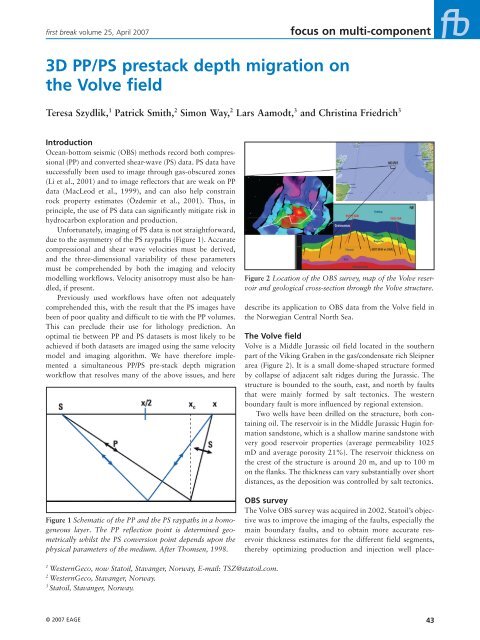
first break volume 25, April 2007
D <strong>PP</strong>/<strong>PS</strong> <strong>prestack</strong> <strong>depth</strong> <strong>migration</strong> on
the Volve field
Introduction
Ocean-bottom seismic (OBS) methods record both compressional
(<strong>PP</strong>) and converted shear-wave (<strong>PS</strong>) data. <strong>PS</strong> data have
successfully been used to image through gas-obscured zones
(Li et al., 2001) and to image reflectors that are weak on <strong>PP</strong>
data (MacLeod et al., 1999), and can also help constrain
rock property estimates (Özdemir et al., 2001). Thus, in
principle, the use of <strong>PS</strong> data can significantly mitigate risk in
hydrocarbon exploration and production.
Unfortunately, imaging of <strong>PS</strong> data is not straightforward,
due to the asymmetry of the <strong>PS</strong> raypaths (Figure 1). Accurate
compressional and shear wave velocities must be derived,
and the three-dimensional variability of these parameters
must be comprehended by both the imaging and velocity
modelling workflows. Velocity anisotropy must also be handled,
if present.
Previously used workflows have often not adequately
comprehended this, with the result that the <strong>PS</strong> images have
been of poor quality and difficult to tie with the <strong>PP</strong> volumes.
This can preclude their use for lithology prediction. An
optimal tie between <strong>PP</strong> and <strong>PS</strong> datasets is most likely to be
achieved if both datasets are imaged using the same velocity
model and imaging algorithm. We have therefore implemented
a simultaneous <strong>PP</strong>/<strong>PS</strong> pre-stack <strong>depth</strong> <strong>migration</strong>
workflow that resolves many of the above issues, and here
© 2007 EAGE
focus on multi‑component
Teresa Szydlik, 1 Patrick Smith, 2 Simon Way, 2 Lars Aamodt, 3 and Christina Friedrich 3
Figure 1 Schematic of the <strong>PP</strong> and the <strong>PS</strong> raypaths in a homogeneous
layer. The <strong>PP</strong> reflection point is determined geometrically
whilst the <strong>PS</strong> conversion point depends upon the
physical parameters of the medium. After Thomsen, 1998.
1 WesternGeco, now Statoil, Stavanger, Norway, E-mail: TSZ@statoil.com.
2 WesternGeco, Stavanger, Norway.
3 Statoil, Stavanger, Norway.
Figure 2 Location of the OBS survey, map of the Volve reservoir
and geological cross-section through the Volve structure.
describe its application to OBS data from the Volve field in
the Norwegian Central North Sea.
The Volve field
Volve is a Middle Jurassic oil field located in the southern
part of the Viking Graben in the gas/condensate rich Sleipner
area (Figure 2). It is a small dome-shaped structure formed
by collapse of adjacent salt ridges during the Jurassic. The
structure is bounded to the south, east, and north by faults
that were mainly formed by salt tectonics. The western
boundary fault is more influenced by regional extension.
Two wells have been drilled on the structure, both containing
oil. The reservoir is in the Middle Jurassic Hugin formation
sandstone, which is a shallow marine sandstone with
very good reservoir properties (average permeability 1025
mD and average porosity 21%). The reservoir thickness on
the crest of the structure is around 20 m, and up to 100 m
on the flanks. The thickness can vary substantially over short
distances, as the deposition was controlled by salt tectonics.
OBS survey
The Volve OBS survey was acquired in 2002. Statoil’s objective
was to improve the imaging of the faults, especially the
main boundary faults, and to obtain more accurate reservoir
thickness estimates for the different field segments,
thereby optimizing production and injection well place-

focus on multi‑component first break volume 25, April 2007
Table 1 Seismic processing sequence prior to <strong>depth</strong> imaging.
ment. OBS was chosen over marine streamer acquisition to
take advantage of improved water-layer multiple attenuation by
combining geophone and hydrophone measurements, and for
the superior illumination properties given by its wider azimuth
range. The availability of <strong>PS</strong> data was not included in the cost
benefit analysis prior to acquisition, as it was not expected to
contribute significantly to structural image quality or the interpretation
of the reservoir distribution.
The survey was acquired using an inline shooting geometry.
It comprises six swaths of four-component data, with each
swath comprising data from two 6 km long Nessie-4C cables
laid on the seabed with 400 m spacing, and 25 dual source
lines shot with 100 m separation. There was an 800 m moveup
between swaths. The source area covered roughly 70 km 2 and
the receiver area about 27 km 2 .
Seismic processing of OBS data
After acquisition, the OBS data was processed through a fairly
standard <strong>PP</strong> pre-stack time imaging flow. At that time a successful
pilot study was performed to demonstrate the potential
benefits of using a simultaneous <strong>PP</strong>/<strong>PS</strong> pre-stack <strong>depth</strong> imaging
approach, and Statoil therefore decided to process the full dataset
using this workflow. The project is the subject of this paper.
The pre-imaging seismic processing is summarized in Table 1.
Figure 3 The model-building workflow for a single layer of
the <strong>depth</strong> model.
Prior to PZ combination, Z to P component frequency, phase
and amplitude matching was applied. The <strong>PS</strong> dataset was created
by rotation of the horizontal inline and crossline geophone
components into the source-receiver (radial) direction (Gaiser
1999). The pre-processing of the <strong>PP</strong> and the <strong>PS</strong> data includes
standard wavelet processing, noise and multiple attenuation
techniques. This data was input to the simultaneous <strong>depth</strong>
imaging workflow.
Simultaneous <strong>PP</strong>/<strong>PS</strong> pre‑stack
<strong>depth</strong> imaging workflow
The <strong>PP</strong> and <strong>PS</strong> <strong>depth</strong> imaging is driven by a common <strong>depth</strong>domain
earth model. This model is layer-based, and each layer
comprises a number of spatially variant attributes:
n Vertical compressional velocity (Vp) at the top of the layer
n Vp <strong>depth</strong> gradient
n Vertical shear velocity (Vs) at the top of the layer
n Vs <strong>depth</strong> gradient
n Thomsens polar anisotropy parameters (epsilon and delta)
The velocity model is built using a layer-stripping approach.
Each layer is updated using a combination of layer-based tomography
and <strong>migration</strong> scanning, constrained by well data such
as compressional and shear sonic logs, check shot data, etc. For
this particular project, we used spatially invariant anisotropy
parameters and gradients within each layer.
On the Volve project, compressional sonic log and check
shot data were available for five wells. We also had shear sonic
log data for two wells, but chose not to use this for velocity
modelling, as we were uncertain about their accuracy. The
layer boundaries, chosen by examining the sonic logs and initial
velocity analyses made from the seismic data, defined the major
interval velocity contrasts and changes in velocity gradient.
The velocity modelling workflow for a given layer is shown
in Figure 3. The model is first flooded from the top of the
current layer downwards with an initial estimate of Vp. The
epsilon and delta values are initially set to zero for the shallow
layers, but for the deeper layers, initial estimates are used, based
Figure 4 The Vp/Vs ratio derived from the Volve <strong>depth</strong> model
(left) compared with the high-resolution Vp/Vs ratio derived
using the method of Nickel et al. (2004).
© 2007 EAGE

first break volume 25, April 2007
© 2007 EAGE
focus on multi‑component
Figure 5 Vertical slices through the <strong>depth</strong> model showing colour-coded Vp and Vs properties. For each layer listed are velocity
gradients dv/dz [m/s/m] and Thomsen anisotropy parameters delta and epsilon.
Figure 6 Figure 6 shows, for well A, the sonic log velocities, Vp extracted from the velocity model at the well location, and
<strong>depth</strong> migrated <strong>PP</strong> and <strong>PS</strong> data as a composite seismic section crossing the well location.

focus on multi‑component first break volume 25, April 2007
on the layers above. The <strong>PP</strong> data is then migrated. We evaluate
the flatness of the resulting common image point (CIP)
gathers, and the <strong>depth</strong> tie between the seismic and well data.
Vp, epsilon, and delta are updated as necessary and a second
<strong>migration</strong> performed. The process is repeated until we are
happy with the gather flatness and <strong>depth</strong> tie with the wells.
We then generate Vs for the current layer, usually by assuming
a Vp/Vs ratio based on well data or other information, and
migrate the <strong>PS</strong> data. Vs is updated to achieve a zero-offset
<strong>depth</strong> tie with the migrated <strong>PP</strong> data, and to the wells. The data
are remigrated and the process repeated until we are happy
with the <strong>depth</strong> ties. We then evaluate the flatness of the <strong>PS</strong>
CIP gathers, and update the anisotropy parameters, iterating
as necessary. Next we remigrate the <strong>PP</strong> data with the revised
anisotropy parameters to ensure that the <strong>PP</strong> gathers are
optimally flattened. Because the <strong>PP</strong> data are less sensitive to
anisotropy than <strong>PS</strong>, the anisotropy parameters which flatten
the <strong>PS</strong> gathers are normally also appropriate for the <strong>PP</strong> data.
We can then move on to the next layer.
Seven layers were sufficient to represent the subsurface
down to Middle Jurassic. Optimization of each layer prop-
Figure 7 Modelled versus measured Vp and Vs in well B.
6
erty required up to three <strong>depth</strong> <strong>migration</strong> iterations.
It is obviously vital that the same reflection is interpreted
on both the <strong>PP</strong> and <strong>PS</strong> data, something that is not always
straightforward. Our top-down method means that the <strong>PS</strong>
data for the next iteration can be quite accurately imaged
using the current model and an assumed Vp/Vs ratio for
the next layer, which greatly eases correlation of <strong>PP</strong> and <strong>PS</strong>
reflectors. It can also be helpful to use <strong>PP</strong> and <strong>PS</strong> synthetic
seismograms, based on well data, to evaluate the expected
difference in phase and amplitude character of a given reflector
on the two datasets.
The <strong>depth</strong> imaging workflow ensures that the <strong>PP</strong> and <strong>PS</strong>
data match at the velocity model layer boundaries, but does
not guarantee a tie in between. The automated <strong>PS</strong> to <strong>PP</strong> event
registration and matching algorithm developed by Nickel et al.
(2004) can be used to align the datasets in a high frequency
manner, generating, as a by-product, a high resolution Vp/Vs
ratio cube (Figure 4) that is also a valuable interpretation
attribute. The alignment assures consistency between attributes
extracted from the <strong>PP</strong> and <strong>PS</strong> cubes, and is a prerequisite for
simultaneous pre-stack inversion.
Figure 8 Comparison of the <strong>PP</strong> dataset after <strong>prestack</strong> time
<strong>migration</strong> and <strong>prestack</strong> <strong>depth</strong> <strong>migration</strong>. Note improvement
in the fault definition on the <strong>prestack</strong> <strong>depth</strong>-migrated dataset
(a). Time slices showing better reservoir image after <strong>prestack</strong>
<strong>depth</strong> <strong>migration</strong> (b).
A
B
© 2007 EAGE

first break volume 25, April 2007
Simultaneous <strong>PP</strong>/<strong>PS</strong> pre‑stack <strong>depth</strong> imaging results
Figure 5 shows vertical slices through the final model, colourcoded
by Vp and Vs. Epsilon and delta are listed for each layer.
It is obvious that the Vp/Vs ratio varies spatially and with
<strong>depth</strong>.
Figure 6 shows the sonic log velocities for well A, Vp
extracted from the velocity model at the well location, and
<strong>depth</strong>-migrated <strong>PP</strong> and <strong>PS</strong> data as a composite seismic section
crossing the well position. The <strong>PP</strong> seismic ties the <strong>depth</strong> markers
at the well location, and the Vp profile agrees well with the
sonic velocities. By enforcing a <strong>depth</strong> tie between <strong>PP</strong> and <strong>PS</strong>
during velocity model building, we implicitly achieve a <strong>depth</strong>
tie between <strong>PS</strong> and the wells.
Figure 7 shows compressional and shear sonic logs from
well B, overlain by Vp and Vs extracted from the final velocity
model at the well location. We see an excellent tie, even though
the shear sonic logs were not used during modelling.
Comparison of <strong>PP</strong> pre-stack time and pre-stack <strong>depth</strong>
migrated datasets shows that the pre-stack <strong>depth</strong> <strong>migration</strong> better
images the subtle faulting that is characteristic of this area
(Figure 8(a)) and reservoir structure (Figure 8(b)). However the
real value of the approach is seen when the <strong>PP</strong> and <strong>PS</strong> <strong>depth</strong>
migrated datasets are compared (Figure 9). The correlation of
reflections between the two datasets is unambiguous over much
of the section. We see differences in character between some
reflections. The <strong>PS</strong> and <strong>PP</strong> CIP gathers (Figure 10) show similar
differences, which are not related to poor imaging, but are
indicative of genuine differences in <strong>PP</strong> and <strong>PS</strong> reflectivity, and
which presumably carry information about rock properties.
The interpretability of the <strong>PS</strong> data below the Base Cretaceous
unconformity still does not match that of the <strong>PP</strong> cube (Figure 9).
This is perhaps unsurprising; the shear impedance contrast of
the reservoir interval is quite small and the reservoir structure
is complex. <strong>PS</strong> imaging is much more reliant on the accuracy of
the velocity model than <strong>PP</strong> imaging, and so small inaccuracies
in the model affect the <strong>PS</strong> data to a greater extent.
Conclusions
The <strong>depth</strong> imaging workflow presented here has been used
successfully on a number of projects. Application to the Volve
OBS data gives a <strong>PS</strong> dataset that unambiguously ties the <strong>PP</strong>
dataset in <strong>depth</strong> and character down to BCU level. This was
achieved by determining an accurate polar anisotropic compressional
and shear velocity model of the subsurface using all
available data.
Currently many OBS acquisitions are justified solely on
the likelihood of improved <strong>PP</strong> data quality. We believe that the
workflow presented will help further extend the applicability
of OBS data to lithology and fluid prediction, and that the
availability of <strong>PS</strong> data should be weighted more heavily when
seismic data acquisition decisions are being made.
References
Xiang-Yang Li, Hengchang Dai, Mueller, M.C., and Barkved,
O.I. [2001] Compensating for the effects of gas clouds on C-
focus on multi‑component
Figure 9 Comparison of the <strong>PP</strong> and <strong>PS</strong> <strong>depth</strong>-migrated results
in <strong>depth</strong>.
Figure 10 Comparison of CIP <strong>depth</strong> gathers from the <strong>PP</strong> and
<strong>PS</strong> datasets.
wave imaging: A case study from Valhall. The Leading Edge,
20, 1022.
Gaiser, J.E. [1999] Applications for vector coordinate systems of
3-D converted-wave data. The Leading Edge, 18, 1290-1300.
MacLeod, M., Hanson, R., Hadley, M., Reynolds, K., Lumley,
D., McHugo, S., and Probert, T. [1999] The Alba Field
OBC seismic survey. 69 th SEG Annual International Meeting,
Expanded Abstract, 18, 725.
Nickel, M. and Sonneland, L. [2004] Automated <strong>PS</strong> to <strong>PP</strong> event
registration and estimation of a high-resolution Vp-Vs ratio
volume. 74 th SEG Annual International Meeting, Expanded
Abstract, 23, 869.
Thomsen, L. [1998] Converted-wave reflection seismology
over anisotropic, inhomogenous media. 68 th SEG Annual
International Meeting, , Extended Abstracts, 2048-2051.
Özdemir, H., Ronen, S., Olofsson, B., Goodway, B., and Young,
P. [2001] Simultaneous multicomponent AVO inversion. 71 st
SEG Annual International Meeting, Expanded Abstract, 20,
269.
© 2007 EAGE 7