BER calculation for AWGN channel
BER calculation for AWGN channel
BER calculation for AWGN channel

Create successful ePaper yourself
Turn your PDF publications into a flip-book with our unique Google optimized e-Paper software.
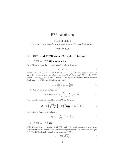
<strong>BER</strong> <strong>calculation</strong><br />
Vahid Meghdadi<br />
reference: Wireless Communications by Andrea Goldsmith<br />
January 2008<br />
1 SER and <strong>BER</strong> over Gaussian <strong>channel</strong><br />
1.1 <strong>BER</strong> <strong>for</strong> BPSK modulation<br />
In a BPSK system the received signal can be written as:<br />
y = x + n (1)<br />
where x ∈ {−A, A}, n ∼ CN (0, σ 2 ) and σ 2 = N 0 . The real part of the above<br />
equation is y re = x + n re where n re ∼ N (0, σ 2 /2) = N (0, N 0 /2). In BPSK<br />
constellation d min = 2A and γ b is defined as E b /N 0 and sometimes it is called<br />
SNR per bit. With this definition we have:<br />
So the bit error probability is:<br />
γ b := E b<br />
N 0<br />
= A2<br />
N 0<br />
= d2 min<br />
4N 0<br />
(2)<br />
P b = P {n > A} =<br />
∫ ∞<br />
A<br />
1<br />
√<br />
2πσ2 /2 e−<br />
This equation can be simplified using Q-function as:<br />
⎛√<br />
⎞<br />
P b = Q ⎝<br />
d 2 ( )<br />
min ⎠ dmin<br />
(√ )<br />
= Q √ = Q 2γb<br />
2N 0 2N0<br />
where the Q function is defined as:<br />
1.2 <strong>BER</strong> <strong>for</strong> QPSK<br />
Q(x) = √ 1 ∫ ∞<br />
2π<br />
x<br />
x2<br />
2σ 2 /2<br />
(3)<br />
(4)<br />
e − x2<br />
2 dx (5)<br />
QPSK modulation consists of two BPSK modulation on in-phase and quadrature<br />
components of the signal. The corresponding constellation is presented on figure<br />
. The <strong>BER</strong> of each branch is the same as BPSK:<br />
(√ )<br />
P b = Q 2γb (6)<br />
1
Figure 1: QPSK constellation<br />
The symbol probability of error (SER) is the probability of either branch<br />
has a bit error:<br />
(√ )<br />
P s = 1 − [1 − Q 2γb ] 2 (7)<br />
Since the symbol energy is split between the two in-phase and quadrature components,<br />
γ s = 2γ b and we have:<br />
P s = 1 − [1 − Q ( √ γ s )] 2 (8)<br />
We can use the union bound to give an upper bound <strong>for</strong> SER of QPSK. Regarding<br />
figure , condition that the symbol zero is sent, the probability of error is<br />
bounded by the sum of probabilities of 0 → 1, 0 → 2 and 0 → 3. We can write:<br />
P s ≤ Q(d 01 / √ 2N 0 ) + Q(d 02 / √ 2N 0 ) + Q(d 03 / √ 2N 0 ) (9)<br />
= 2Q(A/ √ N 0 ) + Q( √ 2A/ √ 2N 0 ) (10)<br />
Since γ s = 2γ b = A 2 /N 0 , we can write:<br />
P s ≤ 2Q( √ γ s ) + Q( √ 2γ s ) ≤ 3Q( √ γ s ) (11)<br />
Using the tight approximation of Q function <strong>for</strong> z ≫ 0:<br />
Q(z) ≤ 1<br />
z √ 2π e−z2 /2<br />
(12)<br />
we obtain:<br />
P s ≤<br />
3<br />
√ 2πγs<br />
e −0.5γs (13)<br />
Using Gray coding and assuming that <strong>for</strong> high signal to noise ratio the errors<br />
occur only <strong>for</strong> the nearest neighbor, P b can be approximated from P s by P b ≈<br />
P s /2.<br />
2
Figure 2: MPSK constellation<br />
1.3 <strong>BER</strong> <strong>for</strong> MPSK signaling<br />
For MPSK signaling we can calculate easily an approximation of SER using<br />
nearest neighbor approximation. Using figure , the symbol error probability<br />
can be approximated by:<br />
( ) (<br />
dmin 2A sin<br />
π<br />
) (√ )<br />
M<br />
P s ≈ 2Q √ = 2Q √ = 2Q 2γs sin(π/M) (14)<br />
2N0 2N0<br />
This approximation is only good <strong>for</strong> high SNR.<br />
1.4 <strong>BER</strong> <strong>for</strong> QAM constellation<br />
The SER <strong>for</strong> a rectangular M-QAM (16-QAM, 64-QAM, 256-QAM etc) with<br />
size L = M 2 can be calculated by considering two M-PAM on in-phase and<br />
quadrature components (see figure <strong>for</strong> 16-QAM constellation). The error<br />
probability of QAM symbol is obtained by the error probability of each branch<br />
(M-PAM) and is given by:<br />
P s = 1 −<br />
(<br />
1 −<br />
(√ )) 2<br />
2 (sqrtM − 1)<br />
sqrtM Q 3γs<br />
(15)<br />
M − 1<br />
If we use the nearest neighbor approximation <strong>for</strong> an M-QAM rectangular constellation,<br />
there are 4 nearest neighbors with distance d min . So the SER <strong>for</strong><br />
high SNR can be approximated by:<br />
c (16)<br />
In order to calculate the mean energy per transmitted symbol, it can be seen<br />
that<br />
E s = 1 M∑<br />
A 2 i (17)<br />
M<br />
i=1<br />
3
Figure 3: 16-QAM constellation<br />
Modulation P s (γ s ) P b (γ b )<br />
BPSK P b = Q (√ )<br />
2γ b<br />
QPSK P s ≈ 2Q ( √ )<br />
γs P b ≈ Q (√ )<br />
2γ b<br />
MPSK P s ≈ 2Q (√ 2γ s sin ( ))<br />
π<br />
M<br />
P b ≈ 2<br />
log 2 M Q (√ 2γ b log 2 M sin ( ))<br />
π<br />
M<br />
(√ )<br />
(√ )<br />
M-QAM P s ≈ 4Q 3γs<br />
M−1<br />
P b ≈ 4<br />
log 2 M Q 3γb log 2 M<br />
M−1<br />
Table 1: Approximate symbol and bit error probabilities <strong>for</strong> coherent modulation<br />
Using the fact that A i = (a i + b i ) and a i and b i ∈ {2i − 1 − L} <strong>for</strong> i = 1, ..., L.<br />
After some simple <strong>calculation</strong>s we obtain:<br />
E s = d2 min<br />
2L<br />
L∑<br />
(2i − 1 − L) 2 (18)<br />
i=1<br />
For example <strong>for</strong> 16-QAM and d min = 2 the E s = 10. For 64-QAM and d min = 2<br />
the E s = 21.<br />
1.5 conclusion<br />
The approximations or exact values <strong>for</strong> SER has the following <strong>for</strong>m:<br />
(√ )<br />
P s (γ s ) ≈ α M Q βM γ s<br />
(19)<br />
where α M and β M depend on the type of approximation and the modulation<br />
type. In the table the values <strong>for</strong> α M and β M are semmerized <strong>for</strong> common<br />
modulations.<br />
We can also note that the bit error probability has the same <strong>for</strong>m as <strong>for</strong><br />
SER. It is:<br />
(√ )<br />
P b (γ b ) ≈ ˆα M Q ˆβ M γ b (20)<br />
where ˆα M = α M / log 2 M and ˆβ M = β M / log 2 M.<br />
Note: γ s = E s /N 0 , γ b = E b /N 0 , γ b =<br />
4<br />
γs<br />
log 2 M and P b ≈ Ps<br />
log 2 M .
1.6 Appendix<br />
In this appendix the reference curve <strong>for</strong> <strong>AWGN</strong> <strong>channel</strong> is presented in figure<br />
. As we expected , the results <strong>for</strong> BPQK and QPSK are the same.<br />
Gaussian Channel<br />
10 0 E b<br />
/N 0<br />
(dB)<br />
10 −1<br />
BPSK<br />
QPSK<br />
8PSK<br />
16QAM<br />
10 −2<br />
10 −3<br />
<strong>BER</strong><br />
10 −4<br />
10 −5<br />
10 −6<br />
10 −7<br />
10 −8<br />
0 2 4 6 8 10 12 14 16 18<br />
Figure 4: <strong>BER</strong> over <strong>AWGN</strong> <strong>channel</strong> <strong>for</strong> BPSK, QPSK, 8PSK and 16QAM<br />
The following matlab program illustrates the <strong>BER</strong> <strong>calculation</strong>s <strong>for</strong> BPSK<br />
over an <strong>AWGN</strong> <strong>channel</strong>.<br />
%BPSK <strong>BER</strong><br />
const=[1 -1];<br />
size=100000;<br />
iter_max=1000;<br />
EbN0_min=0;<br />
EbN0_max=10;<br />
SNR=[];<strong>BER</strong>=[];<br />
<strong>for</strong> EbN0 = EbN0_min:EbN0_max<br />
EbN0_lin=10.^(0.1*EbN0);<br />
noise_var=0.5/(EbN0_lin); % s^2=N0/2<br />
iter = 0;<br />
err = 0;<br />
while (iter
end<br />
SNR =[SNR EbN0];<br />
<strong>BER</strong> = [<strong>BER</strong> err/(size*iter)];<br />
end<br />
semilogy(SNR,<strong>BER</strong>);grid;xlabel(’E_bN_0’);ylabel(’<strong>BER</strong>’);<br />
title(’BPSK over <strong>AWGN</strong> <strong>channel</strong>’);<br />
The following program uses some advanced functions of matlab to evaluate the<br />
symbol error rate <strong>for</strong> QPSK modulation:<br />
M = 4; % Alphabet size<br />
EbN0_min=0;EbN0_max=10;step=2;<br />
SNR=[];SER=[];<br />
<strong>for</strong> EbN0 = EbN0_min:step:EbN0_max<br />
SNR_dB=EbN0 + 3; %<strong>for</strong> QPSK Eb/N0=0.5*Es/N0=0.5*SNR<br />
x = randint(1000000,1,M);<br />
y=modulate(modem.qammod(M),x);<br />
ynoisy = awgn(y,SNR_dB,’measured’);<br />
z=demodulate(modem.qamdemod(M),ynoisy);<br />
[num,rt]= symerr(x,z);<br />
SNR=[SNR EbN0];<br />
SER=[SER rt];<br />
end;<br />
semilogy(SNR,SER);grid;titel(’Symbol error rate <strong>for</strong> QPSK over <strong>AWGN</strong>’);<br />
xlabel(’E_b/N_0’);ylabel(’SER’);<br />
2 SER and <strong>BER</strong> over fading <strong>channel</strong> 1<br />
2.1 PDF-based approach <strong>for</strong> binary signal<br />
A fading <strong>channel</strong> can be considered as an <strong>AWGN</strong> with a variable gain. The<br />
gain itself is considered as a RV with a given pdf. So the average <strong>BER</strong> can<br />
be calculated by averaging <strong>BER</strong> <strong>for</strong> instantaneous SNR over the distribution of<br />
SNR:<br />
P b (E) =<br />
∫ ∞<br />
0<br />
P b (E|γ)p γ (γ)dγ<br />
The <strong>BER</strong> is expressed by a Q-function as seen in previous chapter:<br />
P b (E) =<br />
∫ ∞<br />
where g = 1 <strong>for</strong> the case of coherent BPSK.<br />
0<br />
Q( √ 2gγ)p γ (γ)dγ (21)<br />
Example 1. Rayleigh fading <strong>channel</strong> with coherent detection:<br />
The received signal in a Rayleigh fading <strong>channel</strong> is of the <strong>for</strong>m:<br />
y = hx + w (22)<br />
1 ”Digital Communication over Fading Channel” by Simon and Alouini<br />
6
where h is the <strong>channel</strong> attenuation with normal distribution h ∼ CN (0, 1) and<br />
n is a white additive noise w ∼ CN (0, N 0 ). The coherent receiver constructs<br />
the following metric from the received signal:<br />
h ∗ y = |h| 2 x + h ∗ w (23)<br />
Using BPSK modulation and since the in<strong>for</strong>mation are real, only the real part<br />
of the equation is of interest. So the following sufficient statistic is used <strong>for</strong><br />
decision at the receiver. { } h<br />
∗<br />
R<br />
|h| y = |h|x + n (24)<br />
The noise n has the same statistics as Rw because h ∗ /|h| = exp(jθ) with θ<br />
uni<strong>for</strong>mly distributed in (0, π), there<strong>for</strong>e n ∼ CN (0, N 0 /2). This equation<br />
shows that we have a normal <strong>AWGN</strong> <strong>channel</strong> with the signal scaled by |h|.<br />
The bit error probability as seen be<strong>for</strong>e <strong>for</strong> this case, given h, will be:<br />
(√ )<br />
P b = Q 2|h|2 γ b<br />
Now, we compute the SER by averaging this <strong>BER</strong> over the distribution of h.<br />
Since h is complex Gaussian, the distribution of r = |h| 2 will be exponential<br />
with:<br />
P r (r) = d (<br />
P (h<br />
2<br />
dr r + h 2 i < r) )<br />
( ∫<br />
= d 2π ∫ √ )<br />
r<br />
1<br />
dr<br />
2π1/2 e−x2 xdxdθ<br />
0<br />
0<br />
= d (<br />
1 − e<br />
−r )<br />
dr<br />
= e −r U(r)<br />
There<strong>for</strong>e the signal-to-noise-ratio distribution γ = |h| 2 γ b will be:<br />
p γ (γ) = 1 γ b<br />
e −γ/γ b<br />
The error probability can be calculated by:<br />
P b =<br />
∫ ∞<br />
0<br />
Q( √ 2γ)p γ (γ)dγ =<br />
∫ ∞<br />
0<br />
Q( √ 2γ) 1 γ b<br />
e −γ/γ b<br />
dγ<br />
Using the following <strong>for</strong>m of Q-function and MGF function, the integral can eb<br />
calculated.<br />
Q(x) = 1 π<br />
p b = 1 2<br />
∫ π/2<br />
x2<br />
exp(−<br />
0 2 sin 2 θ )dθ<br />
( √ )<br />
γb<br />
1 −<br />
1 + γ b<br />
7
Example 2. Consider a SIMO system with L receive antennas. Each branch<br />
has a SNR per bit of γ l and there<strong>for</strong>e the SNR at the output of MRC combiner<br />
is γ t = ∑ L<br />
l=1 γ l. Suppose a Rayleigh <strong>channel</strong>, the pdf of SNR <strong>for</strong> each <strong>channel</strong><br />
will be (supposing i.i.d. <strong>channel</strong>s):<br />
p γl (γ l ) = 1¯γ e−γ l/¯γ<br />
At the output of combiner, the SNR follows the distribution of chi-square (or<br />
gamma) with L degrees of freedom:<br />
1<br />
p γt (γ t ) =<br />
(L − 1)!¯γ L γL−1 t<br />
e −γt/¯γ<br />
The average probability can be calculated using the integration by part and<br />
resulting in the following <strong>for</strong>mula:<br />
( ) L L−1<br />
1 − µ ∑<br />
( L − 1 + l<br />
P b (E) =<br />
2<br />
l<br />
l=0<br />
2.2 MGF-based approach<br />
2.2.1 Binary PSK<br />
) ( 1 + µ<br />
We can use the other representation of Q-function to simplify the <strong>calculation</strong>s.<br />
Q(x) =<br />
∫ ∞<br />
x<br />
)<br />
1<br />
√ exp<br />
(− y2<br />
dy = 1 2π 2 π<br />
There<strong>for</strong>e the equation () can be written as:<br />
P b (E|{γ l } L l=1) = 1 π<br />
∫ π/2<br />
0<br />
∫ π/2<br />
exp(− gγ t<br />
sin 2 φ )dφ = 1 ∫ π/2<br />
π<br />
0<br />
0<br />
2<br />
) l<br />
)<br />
exp<br />
(− x2<br />
2 sin 2 dθ<br />
θ<br />
L∏<br />
l=1<br />
exp(− gγ l<br />
sin 2 )dφ (25)<br />
φ<br />
This <strong>for</strong>m of Q-function is more convenient because it allows us to average<br />
first over the individual distributions of γ l and then per<strong>for</strong>m the integral over<br />
φ.<br />
∫ ∞ ∫ ∞ ∫ ∞<br />
L∏<br />
P b (E) = ... P b ({γ l } L l=1) p γl (γ l )dγ 1 dγ 2 ...dγ L (26)<br />
0<br />
0<br />
Using () in () and changing the order of integration gives:<br />
P b (E) = 1 π<br />
0<br />
∫ π/2<br />
0<br />
l=1<br />
l=1<br />
L∏<br />
(<br />
M γl −<br />
g )<br />
sin 2 dφ (27)<br />
φ<br />
8
2.2.2 MPSK<br />
For MPSK signaling the SER given all the SNRs is:<br />
where g = sin 2 (π/m).<br />
P s (E|{γ l } L l=1) = 1 π<br />
P s (E|{γ l } L l=1) = 1 π<br />
∫ (M−1)π/M<br />
0<br />
∫ (M−1)π/M<br />
0<br />
(<br />
exp − gγ )<br />
t<br />
sin 2 dφ (28)<br />
φ<br />
L∏<br />
l=1<br />
(<br />
exp − gγ )<br />
l<br />
sin 2 dφ (29)<br />
φ<br />
9