ChE 253M Experiment No. 2 COMPRESSIBLE GAS FLOW

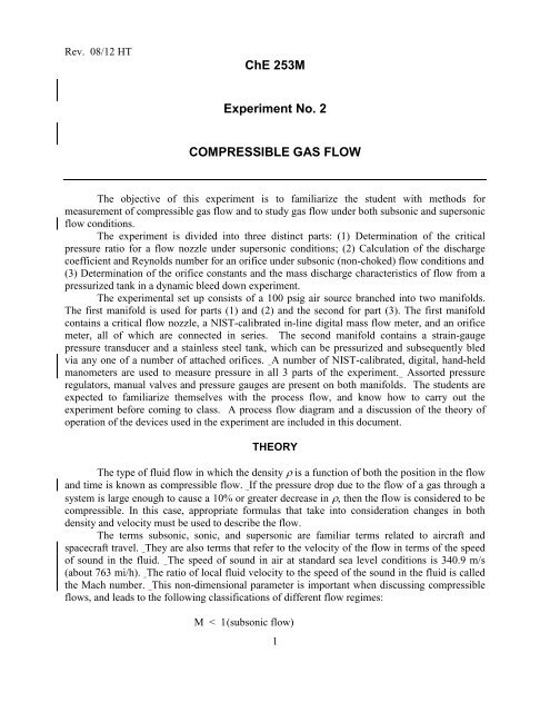
Rev. 08/12 HT
ChE 253M
Experiment No. 2
COMPRESSIBLE GAS FLOW
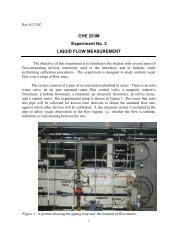
The objective of this experiment is to familiarize the student with methods for
measurement of compressible gas flow and to study gas flow under both subsonic and supersonic
flow conditions.
The experiment is divided into three distinct parts: (1) Determination of the critical
pressure ratio for a flow nozzle under supersonic conditions; (2) Calculation of the discharge
coefficient and Reynolds number for an orifice under subsonic (non-choked) flow conditions and
(3) Determination of the orifice constants and the mass discharge characteristics of flow from a
pressurized tank in a dynamic bleed down experiment.
The experimental set up consists of a 100 psig air source branched into two manifolds.
The first manifold is used for parts (1) and (2) and the second for part (3). The first manifold
contains a critical flow nozzle, a NIST-calibrated in-line digital mass flow meter, and an orifice
meter, all of which are connected in series. The second manifold contains a strain-gauge
pressure transducer and a stainless steel tank, which can be pressurized and subsequently bled
via any one of a number of attached orifices. A number of NIST-calibrated, digital, hand-held
manometers are used to measure pressure in all 3 parts of the experiment. Assorted pressure
regulators, manual valves and pressure gauges are present on both manifolds. The students are
expected to familiarize themselves with the process flow, and know how to carry out the
experiment before coming to class. A process flow diagram and a discussion of the theory of
operation of the devices used in the experiment are included in this document.
THEORY
The type of fluid flow in which the density is a function of both the position in the flow
and time is known as compressible flow. If the pressure drop due to the flow of a gas through a
system is large enough to cause a 10% or greater decrease in , then the flow is considered to be
compressible. In this case, appropriate formulas that take into consideration changes in both
density and velocity must be used to describe the flow.
The terms subsonic, sonic, and supersonic are familiar terms related to aircraft and
spacecraft travel. They are also terms that refer to the velocity of the flow in terms of the speed
of sound in the fluid. The speed of sound in air at standard sea level conditions is 340.9 m/s
(about 763 mi/h). The ratio of local fluid velocity to the speed of the sound in the fluid is called
the Mach number. This non-dimensional parameter is important when discussing compressible
flows, and leads to the following classifications of different flow regimes:
M < 1 (subsonic flow)
1

M = 1 (sonic flow)
M > 1 (supersonic flow)
Interestingly enough, the Mach number has some additional physical meaning. For a
“calorically perfect” gas, the square of the Mach number is proportional to the ratio of kinetic to
internal energy. Therefore, it is a measure of the directed motion of the gas compared to the
random thermal motion of the molecules.
What is perceived as the sense of sound by the brain is in actuality the effect of pressure
fluctuations acting on the ear. These weak vibrations travel as pressure waves, alternate
expansions and contractions, through the surrounding fluid. The velocity of their propagation is
the speed of sound, which can be determined by applying the laws of conservation of mass and
linear momentum across a pressure wave front traveling through a stationary fluid. The process
inside the sound wave is assumed to be isentropic; there are no viscous forces acting on the fluid
and no heat transfer to or from it. This assumption is reasonable since the wave front has an
infinitesimal length and there is not enough time for heat transfer to occur. The flow is therefore
considered to be reversible and adiabatic.
Compressible Flow through Orifice and Venturi Meters
Two types of devices are treated together: orifice and venturi meters. They are both
obstruction meters, and based on the same fundamental principle. The device consists of an
obstacle placed in the path of the flowing fluid that causes localized changes in velocity, and
consequently, in pressure. At the point of maximum restriction, the velocity will be the
maximum and the pressure minimum. A part of this pressure loss is recovered downstream of
the obstruction.
“1” “2”
Flow
Figure 1: Compressible Flow through an orifice
The basic equation for calculating the pressure drop through an orifice or venturi is the Bernoulli
equation,
2
V
gh
P = constant (1)
2g
c
g c
where P is pressure, ρ is fluid density, V is fluid velocity, g is acceleration of gravity, h is height,
and g c is a conversion factor for English units. If subscript “1” refers to the upstream conditions
and subscript “2” to the downstream conditions at the point of pressure measurement, then
2

assuming negligible change in temperature and no change in elevation (flow in a horizontal pipe)
the Bernoulli equation simplifies to,
V
V
P (2)
2 2
1 1 2 2
1
P2
2gc
2gc
For an incompressible fluid such as a liquid, can be assumed to be constant (for a gas is not
constant). If Q is the volumetric flow rate of the liquid, Q = A 1 V 1 = A 2 V 2 , where A 1 and A 2
are the cross-sectional areas at points “1” and “2” where the pressures are measured. Thus we
can write:
2 2
1
Q
1
1
Q
1
P1 P2
2g A 2g A
For a liquid, solving for Q
1
the volumetric flow rate,
c 2 c 1
(3)
Q
A
2 g ( P P ) /
c 1 2 1
1 2 2
1 ( A2 A1)
(4)
However, a gas is compressible so for gases an expansion factor (Y) must be added to the above
equation to compensate for changes in density across the restriction. Also, to account for
pressure losses in the device, a discharge coefficient C d must be introduced. Hence the final
form of the equation governing the volumetric flow rate of a gas through an orifice is :
or
Q
C Y A
2 g ( P P )
c 1 2
1 d 2 4
1(1 )
1 2 c 1 2 1
(5a)
Q CY A 2 g ( P P )
(5b)
4
where = d 2 / d 1 is the ratio of the orifice diameter to the pipe diameter and C C d
1
.
Multiplying by the density upstream of the orifice, we obtain the mass flow rate, w, of the fluid
at any point,
w Q CY A gc
( P )
(6)
1 1
2
2
1 1
P2
For the flow of liquid, the expansion factor, Y is unity and for gases Y can be calculated from
1
4
2 1
r
1
Y r
(7)
4
1
1
r 1
r
2
3

where r = P 2 / P 1 and = c p / c v is the specific heat ratio, equal to = 1.4 for air. For values of
4
less than 0.25, aproaches zero and the last bracketed term in the above equation approaches 1
so that the equation simplifies to
Y
r
2
1
1
r
1
1
r
(8)
Values of Y as a function of r, and can be calculated either directly from equations 7 or 8 or
can be read from a graph that readily displays computed values of Y as a function of these
parameters (see appendix). Finally, substituting equation 8 into the mass flow rate equation 6
and simplifying using the ideal gas law yields the general equation for subsonic (non-choked)
flow of an ideal gas through an orifice
w C P A
1
2
2gcM
RT
1
P
2
1
P1
2
P2
P1
1
(9)
Critical Flow Nozzle – Choked Flow
Consider the case where a compressible fluid is expanded from a given pressure “1” to a
lower downstream pressure “2” in a carefully-machined nozzle of the sort depicted in Figure 1.
As the downstream pressure, or back pressure, is lowered, the mass flow rate and the fluid
velocity increase until the velocity in the throat of the nozzle becomes sonic. The value of r = P 2
/ P 1 at which the speed of sound is reached is called the critical pressure ratio r c and depends
only on (ratio of specific heat capacities) and (ratio of nozzle to pipe diameters).
For ≤ this is given by
1
2
r
c
= 0.528 for air ( (10)
1
As long as the flow in the throat is sonic, the mass flow rate through the nozzle is
constant for a given value of upstream pressure, and the flow is said to be choked. Any further
lowering of the downstream pressure does not increase the throat velocity above sonic.
However, if the downstream pressure is raised above this critical value, the velocity at the throat
goes subsonic and choked flow conditions no longer exist (Figure 2).
4

Mass
Flow
Rate
Air
Velocity
Sonic Velocity
1127 ft/s @ 68 ºF
P 1 = Constant
1
2
r c
1
0.528 for air
1
P 2 / P 1
0
Figure 2: For a fixed inlet pressure P 1 , the air velocity and mass flow rate are limited
(choked) below the critical pressure ratio.
During choked or critical flow conditions, the flow rate can be increased only by
increasing the upstream pressure. When the pressure ratio r reaches the critical value r c of
equation 10, then the mass flow rate for choked flow in equation 9 reduces to:
5
( 1)
( 1)
gc M 2
w C A P . (11)
RT1 1
Since C, A, g c , , M, R are constant for a given nozzle and gas, they can be combined to result
the following simplified relation:
w K P
,
T
gcM
2
K CA
R 1
1) /( 1)
1/ 2
It turns out that K (and hence C) is a weak function of P (a plot of K versus P for the
critical flow nozzle used in this experiment is attached in the appendix). Therefore, at choked
flow the only measurements required to determine the flow rate through the critical flow nozzle
are the upstream pressure and temperature. Finally, note than when a downstream diffuser
(divergent) recovery section is added to the flow nozzle (better known as critical flow venturi
nozzle), the value for the critical pressure ratio r c is no longer the theoretical value given in
equation 10, but ranges from 0.80 to 0.95 depending on the design. (Note: the flow nozzle in this
experiment does have such a diffuser recovery section).
List of Variables and Constants
Q 1 = upstream volumetric flow rate, ft³/s
w = mass flow rate at any point, lb m /s
C d = coefficient of discharge, dimensionless
C = orifice flow coefficient, dimensionless
Y = expansion factor, dimensionless
(12)

A 1 = cross-sectional area of the pipe, ft²
A 2 = cross-sectional area of the orifice hole, ft²
d 1 = diameter of the pipe, ft
d 2 = diameter of the orifice hole, ft
β = ratio of orifice hole diameter to pipe diameter, dimensionless
V 1 = upstream fluid velocity, ft/s
V 2 = fluid velocity through the orifice hole, ft/s
P 1 = fluid upstream absolute pressure, lb f /ft 2
P 2 = fluid downstream absolute pressure, lb f /ft 2
ρ 1 = upstream fluid density, lb m /ft³
R = Universal Gas constant, 1545 ft lb f / lbmole °R
g c = dimensional constant, 32.2 lb m ft/sec 2 lb f
Dynamic Pressure Bleed Down Rate Measurement
An important application of choked flow is in calculating accidental release flow rates
from pressurized gas systems. Every pressure tank in a chemical plant is connected to a flare
system through a pressure relief valve. This is to ensure that if a pressure vessel becomes overpressurized,
the tank can relieve itself without rupturing. In most cases the flow from the tank
passes through a restriction where the flow is sonic and it is the diameter of the restriction which
determines how fast gas can escape. Gas flow is sonic if the upstream absolute pressure is
approximately twice the downstream pressure (approx. 28 psia when released to the atmosphere).
The experimental tank, rated at 1,800 psig, has an internal volume of 10.3 L. The air is
released through orifices having diameters of 0.030, 0.040, and 0.055 inches plus an orifice of
unknown diameter to be determined experimentally. The rate of pressure fall-off through these
three orifices is measured with a pressure transducer that is connected to a computer-based data
acquisition system. As we have seen earlier, for a critical flow orifice
( 1)
( 1)
gc M 2
w C A P
(11)
RT1 1
We can simplify this equation in a manner similar to what we did in equation 12. If air is
discharged at constant upstream temperature T 1 then the equation can be simplified to
w
dm
Kd
dt
2
P
(13)
so that the mass flow rate is only a function of the pressure P and orifice diameter d, and all other
variables are included in the orifice constant K. Since air is an ideal gas,
PV
m
nRT RT so that
M
PVM
m (14)
RT
6

and differentiation yields
dm VM dP . (15)
dt RT dt
Substituting back into (13),
VM dP 2
Kd P
RT dt
dP
P
2
Kd RT
VM
dt
P
P0
dP
P
t
t0
2
Kd RT
VM
dt
2
Kd RT
ln P t + constant
VM
2
ln P K'
d t + constant (16)
In this part of the experiment, you will use Equation 16 to determine K' based on your
experimental data for the three orifices provided and then use this value to determine the
diameter of an unknown orifice.
Finally, if we assume that our process is adiabatic and frictionless, then the discharge of the gas
through the orifice is an isentropic expansion of an ideal gas for which
P
constant (17)
For a tank with constant volume, the density is proportional to the mass of the gas inside the
tank and equation 17 can be re-arranged to yield a simple relation between the pressure in the
tank and the mass fraction f m m0
of fluid remaining,
P P0
f
(18)
7

Pressure And Flow Measuring Devices Used in this Experiment
Bourdon Gauge
This very common gauge operates on the principle that the deflection or deformation in a
spiral metal tube can be related to the balance of pressure and elastic forces. The Bourdon tube
is initially coiled in a "C" shaped arc. The tube is sealed at one end and open to the pressure to
be measured at the other. As the pressure increases, the tube deforms, and the motion is
transmitted to a dial indicator by means of a mechanical linkage. Note that in this experiment, the
bourdon gauge is used only as a visual indicator – the NIST-calibrated Digital Handheld
Manometer described below will be used for recording pressure data to be used in your
calculations.
Schaevitz Strain Gauge Transducer
Whereas the bourdon gauge discussed above produces a direct measurement of the
applied pressure via its mechanical linkage and dial indicator, the Schaevitz strain gauge outputs
a voltage signal that is proportional to the applied pressure. This is because the Schaevitz strain
gauge is a transducer. Broadly defined, a transducer is a device, usually electrical, electronic, or
electro-mechanical, that senses or converts a signal from one form to another. In our case, the
strain gauge converts a physical signal (pressure) into an analog signal (voltage). The most
common type of strain gauge consists of an insulating flexible backing which supports a metallic
foil pattern. As pressure is applied, the foil is deformed, causing its electrical resistance to
change. This resistance change, usually measured using a Wheatstone bridge, is related to the
applied strain. Another popular class of strain gauge transducers employs a piezoelectric-type
element. Application of pressure causes it to deform and generate a small potential that is
proportional to the applied pressure.
Differential Manometer
This instrument consists of a simple U-tube about half full of a liquid (in this case, water)
of known density. The two ends of the tube can be connected to the two pressure sources. The
height difference in the liquid column is then proportional to the pressure differential.
Digital Handheld Manometer (NIST Calibrated)
Just like the Schaevitz gauge, this is also a strain gauge transducer but here the strain element is
not a metallic foil but a semiconductor, usually a piece of crystal silicon. Application of pressure
on semiconductor materials such as silicon and germanium causes a proportional change in the
resistance of these materials, a phenomenon known as the piezoresistive effect.
Digital Mass Flow Meter (NIST Calibrated)
The stream of gas entering the Mass Flow transducer is split by shunting a small portion of the
flow through a capillary stainless steel sensor tube. The remainder of the gas flows through the
primary flow conduit. According to principles of fluid dynamics the flow rates of a gas in the
two laminar flow conduits are proportional to one another. Heat flux is introduced at two
sections of the sensor tube by means of precision wound heater sensor coils. As the gas flows
inside the sensor tube, heat is carried by the gas stream from the upstream coil to the downstream
coil windings. The resultant temperature-dependent resistance differential is detected by the
electronic control circuit and the measured gradient at the sensor windings is linearly
proportional to the mass flow rate taking place.
8

PROCEDURE
In addition to the various gauges listed above, the manifold assembly for parts (1) and (2)
includes a main ball valve that supplies air pressure and three gate valves. See the Appendix of
this document for a detailed schematic. In Manifold A, these valves regulate the pressures in the
various parts of the system as follows :
Valve 1A (Pressure Regulator) is located upstream of the critical flow nozzle and
regulates the pressure (P 1 ) upstream to the nozzle. Under choked flow conditions, the
mass flow rate through the system is a function of this pressure and temperature only.
Valve 2A is located downstream of of the critical flow nozzle next to a turbine flow
meter that is not used in this experiment. It regulates the back pressure (P 2 ) of the
nozzle. To ensure choked flow, P2 must be kept below its critical value.
Valve 3A is located downstream of a rotameter not used in this experiment. This valve
should stay open throughout the experiment.
1. Determination Of The Critical Pressure Ratio For Choked Flow And Calibration
Of Critical Flow Nozzle (CFN):
1) Record the atmospheric temperature and pressure. The Teaching Assitant will demonstrate
the use of the barometer used to measure ambient pressure.
2) Set P 1 at 90 psig by adjusting valve 1A (the pressure regulator). Open valves 2A and 3A
completely.
3) Allow 1-2 minutes for the digital mass flow meter to stabilize and record this Q DFM value .
Also record the temperature (T 1 ) upstream to the nozzle.
4) Increase the backpressure (P 2 ) to 10 psig by setting valve 2A appropriately and record the
new flowrate (again, allow enough time for the reading to stablize).
5) Continue to raise the backpressure (P 2 ) in increments of 5 psig and note the point at which
the digital mass flow meter reading begins to change. The corresponding value of P 2 is the
critical backpressure for the given value of P 1 . When P 2 is greater than this critical value,
the flow through the throat is no longer sonic and decreases as P 2 increases.
6) Determine the critical backpressure for the CFN at an upstream pressure (P 1 ) of 70, 50 and
30 psig and close valve 1A when you are finished.
2. Discharge Coefficient For The Orifice Meter
Open valves 2A and 3A completely. Make sure the manometer is about half-full of water and
open the turn valves on the sides of the orifice to allow the pressure to reach the differential
manometer. Set P 1 (by adjusting valve 1A) such that the manometer P is 2 inches H 2 O.
9

Record this P 1 , T 1 and flow rate Q DFM for this setting. Repeat for P = 4 and 6 inches H 2 O.
When you are finished, make sure you close the turn valves on the sides of the orifice and the
main ball valve that supplies air pressure to the manifold.
3. Dynamic Pressure Bleed Down Rate Measurement
NOTE: You can save your data on a USB memory stick or in your UT webspace account
The manifold assembly B for this part consists of the main valve that supplies air pressure, plus:
Valve 1B is a pressure regulator that controls the air pressure into the system
Valve 2B is a manual ball valve that controls the air pressure to the digital manometer
Valve 3B is a manual ball valve upstream of the Schaevitz Strain Gauge transducer
Valve 4B is a manual ball valve downstream of Schaevitz Strain Gauge transducer
Valve 5B is a manual gate valve upstream of the tank. Leave this valve open at all times.
(i) Calibration of the Schaevitz Strain Gauge transducer
First you need to calibrate the Schaevitz Strain Gauge transducer (output in millivolts) against
the NIST-calibrated handheld digital manometer (output in psig).
1. Make sure the 10V DC power supply located behind the computer (used to power the
Schaevitz Strain Gauge transducer) is switched on and then start the Dell computer. Login as
“Fun Lab” and double click the icon on the desktop labeled “Tank Bleeddown.vi”. This is a
LabView based program written specifically to control the data acquisition process, and
continuously displays the voltage output from the Schaevitz Strain Gauge transducer.
2. Verify that Valves 2B and 3B are open and Valve 4B is closed (NO air going to the tank).
Open the main manual ball valve that supplies air pressure to the manifold, and adjust the
pressure regulator (Valve 1) until the pressure reading on the NIST-calibrated handheld
digital manometer is ~10 psig. Read the corresponding voltage output from the Schaevitz
Strain Gauge transducer via the LabView program on the computer.
3. Repeat the process in steps of 10 psig until you reach a final pressure of 90 psig. You now
have 9 points of Pressure vs. mV to obtain a calibration curve.
(ii) Bleed Down Experiment
4. You are now ready to fill the tank with air. First make sure all the orifices attached to the
tank are closed and close valve 2B (digital manometer off-line). Increase the line pressure to
~95 psig, and open valve 4B to fill the tank. You should hear the air filling the tank. When
it stops, close valve 3 so that air does not refill the tank while it is discharging.
5. On the computer you should see the voltage reading on the graph display increase as the tank
fills up and then plateaus when the pressure has stabilized. You may also change the rate at
which data are collected via the “Data Collection Rate” control. Typically, you should select
a slow data collection rate for small orifices and a fast data collection rate for the larger
10

orifices. Once you have selected a data collection rate, click the “Save Data” button and
enter a filename for the bleed down trial. The voltage data is saved in an EXCEL
spreadsheet file in the directory C:\DATA\.
6. The transducer voltage should show up immediately and begin plotting on the screen. Keep
in mind that the orifice bleed down coefficient describes the pressure over time only while
the orifice is open. Data collected while the orifice is closed is useless for such an analysis.
Therefore you should disregard data that is collected after the orifice is closed.
7. Wait for a few seconds until you save a baseline pressure reading from the tank and then
open one of the orifice valves (you will be doing 3 runs - it doesn’t matter which one you do
first). Then, allow the pressure to drop to approximately 30 psig by monitoring the pressure
reading on the small gauge at the side of the tank. When the pressure has reached close to 30
psig, close the orifice valve and on the computer click the button labeled “Writing to data file
– click again to stop writing.” The program resets and is now ready for a new acquisition –
you do not have to press the red stop button on the software after each run, only at very end
of the experiment.
8. Repeat the above process for the two other orifices by simply opening valve 3B to fill up the
tank again and close it after the pressure inside the tank has stabilized. Also, do one trial
where the 0.030” and 0.040” orifices are simultaneously opened and a run for the orifice of
unknown diameter which you will determine in this experiment. You should end up with a
total of 5 bleed down runs.
Note: CFN= Critical Flow Nozzle
DFM=Digital Mass Flow Meter
Data Analysis
1. CFN: Estimate within ± 2 psi the value of P 2 for which sonic flow occurs at the throat
(describe clearly how you reached this value; plotting your data similar to Figure 1 might
help), and tabulate the critical pressure ratios r c = P 2 / P 1 to calculate an overall average.
Compare your result with the CFN manufacturer’s claim that “The diffuser provides efficient
recovery allowing critical flow to be maintained at inlet to exit pressure ratios (P l / P 2 ) as low
as 1.2”.
2. Determine the calibration equation of W DFM (NIST-Calibrated Standard) vs. W CFN. A
manufacturer’s performance curve is attached in the appendix for the CFN. Compute 95%
confidence limits, and show the confidence intervals on the graph. Discuss the
accuracy/precision of the CFN compared to the DFM standard.
3. Orifice: Calculate the discharge coefficient and the Reynolds number of the flow for each
value of P. Compare these values with the values obtained from published data in Perry’s
Handbook (see appendix for a copy of this graph).
4. Tank Bleed Down: Use JMP to produce the following 5 graphs (EACH with confidence
limits) showing slope, intercept, and confidence limits are expected. In your appendix, show
sample calculations for the slope, intercept, and confidence limits for any ONE of these 5
runs:
11

Ln (P) vs. t for 0.030” orifice
Ln (P) vs. t for 0.040” orifice
Ln (P) vs. t for 0.055” orifice
Ln (P) vs. t for 0.030” and 0.040” orifices opened simultaneously
Ln (P) vs. t for the unknown orifice
Finally: For your raw data, PLEASE do not include several pages of the raw P vs. t data
from the computer. Instead show all your P vs. t data for all orifices on a single excel P
vs. t plot and clearly indicate which curve corresponds to which orifice.
5. Make a single plot for all 3 orifices [0.030”, 0.040”, and 0.055”] for the exponential drop of
mass of air remaining in the tank m versus time. Normalize these graphs such that at t=0, P 0
= 90 psig and P final = 30 psig. Calculate the absolute (in lbs) and relative (% of initial) amount
of gas escaped from each orifice during this time. (Hint: Use ideal gas law for m 0 and Eq.18
for the mass fraction remaining)
6. Determine the average experimental K’ values from the four bleed-down trials (the three
individual orifices plus the combination) including its confidence interval.
7. Calculate the diameter of the unknown orifice and the error on this calculation.
8. Compare the slope of the simultaneous discharge of the 0.030” and 0.040” orifices to (i) the
sum of the slopes for the 0.030” and 0.040” individual orifice discharges and (ii) the sum of
the slopes for the 0.030” and 0.055” individual orifice discharges. Does the tank bleed faster
with only the 0.055” orifice open or when the 0.030” + 0.040” combination is open
9. Discuss the importance of the time axes in the bleed down experiments. What is the
consequence of making an error of several seconds in coordinating data acquisition and valve
opening What if you start collecting data late What if you start to collect data early
SAMPLE CALCULATIONS GUIDE
Note : Convert all pressures and temperatures to their absolute values
Orifice Plate (sharp edged) ID = 0.183 inches
Pipe ID = 0.75 inches
1) Calibration of CFN :
Aim: WDFM vs. WCFN
W CFN
W
K P
obtained from P 1 , T 1 and graph in appendix;
T
and since the DTM is essentially open to atmospheric pressure,
DFM
Q DFM
DFM
12

DFM
atm
P
atm
RT
M
atm
air
2) Orifice Meter:
where,
'
2gc
( P
)
Aim: Find the discharge coefficient C d in Q Cd
A2Y
( Q )
' 4 DFM
(1 )
A2 = Area of orifice (refer to data)
Y = expansion factor (Eq. 8 or from graph attached in appendix)
P' = from reading (h)
= d2/d1 (refer to data)
Now, P 2 ' = P atm as the orifice is essentially open to the atmosphere, and P 1 ' = P atm + P'
1
'
1
P ' 1
M air
'
RT 1
P ' 1
M air
RT atm
(P atm P' )M air
RT atm
The Reynolds number is
v
Q
v
A
D or or atm
Re ;
DFM or or
air
13

APPENDIX
Manifold B
Main Valve
Valve
1B
Manifold A
Main Valve
P1 (Bourdon Gauge)
CFN
P2 (Bourdon Gauge)
Valve 2A
Digital
Flow
Meter
Valve 1A
Digital
Manometer
Digital
Manometer
Schaevitz
Press. Transducer
Orifice
Diff.
Manometer
Valve 3A
Valve 3B
Valve 4B
Valve 5B
Orifice
Assembly
Valve 2B
Digital
Manometer
Tank
Gauge
Schematic Of Experimental Setup
14

16