Virtual Screening Workflow - ISP

Virtual Screening Workflow 

Virtual Screening 

Workflow 

Schrödinger Suite 2009 

Schrödinger Press

Virtual Screening Workflow Copyright © 2009 Schrödinger, LLC. All rights 

reserved. 

While care has been taken in the preparation of this publication, Schrödinger 

assumes no responsibility for errors or omissions, or for damages resulting from 

the use of the information contained herein. 

Canvas, CombiGlide, ConfGen, Epik, Glide, Impact, Jaguar, Liaison, LigPrep, 

Maestro, Phase, Prime, PrimeX, QikProp, QikFit, QikSim, QSite, SiteMap, Strike, and 

WaterMap are trademarks of Schrödinger, LLC. Schrödinger and MacroModel are 

registered trademarks of Schrödinger, LLC. MCPRO is a trademark of William L. 

Jorgensen. Desmond is a trademark of D. E. Shaw Research. Desmond is used with 

the permission of D. E. Shaw Research. All rights reserved. This publication may 

contain the trademarks of other companies. 

Schrödinger software includes software and libraries provided by third parties. For 

details of the copyrights, and terms and conditions associated with such included 

third party software, see the Legal Notices for Third-Party Software in your product 

installation at $SCHRODINGER/docs/html/third_party_legal.html (Linux OS) or 

%SCHRODINGER%\docs\html\third_party_legal.html (Windows OS). 

This publication may refer to other third party software not included in or with 

Schrödinger software ("such other third party software"), and provide links to third 

party Web sites ("linked sites"). References to such other third party software or 

linked sites do not constitute an endorsement by Schrödinger, LLC. Use of such 

other third party software and linked sites may be subject to third party license 

agreements and fees. Schrödinger, LLC and its affiliates have no responsibility or 

liability, directly or indirectly, for such other third party software and linked sites, 

or for damage resulting from the use thereof. Any warranties that we make 

regarding Schrödinger products and services do not apply to such other third party 

software or linked sites, or to the interaction between, or interoperability of, 

Schrödinger products and services and such other third party software. 

June 2009

Document Conventions 

In addition to the use of italics for names of documents, the font conventions that are used in 

this document are summarized in the table below. 

Font Example Use 

Sans serif Project Table Names of GUI features, such as panels, menus, 

menu items, buttons, and labels 

Monospace $SCHRODINGER/maestro File names, directory names, commands, environment 

variables, and screen output 

Italic filename Text that the user must replace with a value 

Sans serif 

uppercase 

CTRL+H 

Keyboard keys 

Links to other locations in the current document or to other PDF documents are colored like 

this: Document Conventions. 

In descriptions of command syntax, the following UNIX conventions are used: braces { } 

enclose a choice of required items, square brackets [ ] enclose optional items, and the bar 

symbol | separates items in a list from which one item must be chosen. Lines of command 

syntax that wrap should be interpreted as a single command. 

File name, path, and environment variable syntax is generally given with the UNIX conventions. 

To obtain the Windows conventions, replace the forward slash / with the backslash \ in 

path or directory names, and replace the $ at the beginning of an environment variable with a 

% at each end. For example, $SCHRODINGER/maestro becomes %SCHRODINGER%\maestro. 

In this document, to type text means to type the required text in the specified location, and to 

enter text means to type the required text, then press the ENTER key. 

References to literature sources are given in square brackets, like this: [10]. 

Virtual Screening Workflow 3

4 

Schrödinger Suite 2009



The Virtual Screening Workflow is designed to run an entire sequence of jobs for screening 

large collections of compounds against a particular target. The workflow includes ligand preparation 

using LigPrep, filtering using propfilter on QikProp properties or other structural 

properties, and Glide docking at the three accuracy levels, HTVS, SP, and XP. The design 

allows you to choose which of the stages to include in any run, and which selection of results 

from one stage are passed on to the next. 

Before you run the workflow, you must ensure that receptor is properly prepared, and you must 

generate Glide grids for the receptor. See the Protein Preparation Guide for information on 

protein preparation, and Chapter 4 of the Glide User Manual for information on grid generation. 

The ligand files for the workflow can consist of 2D structures or 3D structures. If you supply 

2D structures, you must run the ligand preparation part of the workflow to convert the structures 

to 3D for docking. This stage runs a LigPrep job, with the standard options for most parts 

of the LigPrep process. You can control some of these options, but if you want to use other 

options, you should run LigPrep on the ligands independently. For more information, see the 

LigPrep User Manual. 

Prefiltering of the ligands can also be performed as part of the workflow. If you want to use the 

Lipinski Rule option, you must run QikProp to obtain the required properties. You can run 

QikProp as part of the workflow, regardless of the ligand source. If you have already run 

QikProp, you do not need to run it again. If you want to specify a custom filter, you can provide 

an input file for ligfilter, which will then filter the structures. For more information on 

ligfilter, see Section D.2.5 of the Maestro User Manual. 

The full workflow includes three docking stages. The first stage performs HTVS docking. The 

ligands that are retained are then passed to the next stage, which performs SP docking; the 

survivors of this stage are passed on to the third stage, which performs XP docking. At each 

stage you can decide how many ligands are kept, and whether all the ionization and tautomeric 

states of each ligand are kept, or only some. 

The workflow is intended to be robust, so that if a subjob fails, the master job will attempt to 

rerun the job a few times before quitting. If the master job fails (for example, due to a system 

failure or network failure) you can restart the job, and it will pick up the calculation from the 

latest point for which it has results and can restart from them. 



The results of multiple runs of the workflow can be merged using the script $SCHRODINGER/ 

utilities/glide_ensemble_merge. Use the -h option for the syntax of this script. 

Running Schrödinger Software 

To run any Schrödinger program on a UNIX platform, or start a Schrödinger job on a remote 

host from a UNIX platform, you must first set the SCHRODINGER environment variable to the 

installation directory for your Schrödinger software. To set this variable, enter the following 

command at a shell prompt: 

csh/tcsh: 

bash/ksh: 

setenv SCHRODINGER installation-directory 

export SCHRODINGER=installation-directory 

Once you have set the SCHRODINGER environment variable, you can start Maestro with the 

following command: 

$SCHRODINGER/maestro & 

It is usually a good idea to change to the desired working directory before starting Maestro. 

This directory then becomes Maestro’s working directory. For more information on starting 

Maestro, including starting Maestro on a Windows platform, see Section 2.1 of the Maestro 

User Manual. 

To run remote jobs, you must have access to a hosts file, named schrodinger.hosts, that 

lists hosts on which Schrödinger software is installed for execution. Details of setting up this 

file can be found in Chapter 6 of the Installation Guide. 

The Virtual Screening Workflow Panel 

The Virtual Screening Workflow panel sets up the input files for LigPrep, QikProp, and Glide 

ligand docking and submits them to the selected host in order. 

To open the Virtual Screening Workflow panel, choose Virtual Screening Workflow from the 

Workflows menu in the main window. 

The main part of the Virtual Screening Workflow panel consists of three tabs for setting up 

virtual screening jobs. The features of these tabs and how to use them are described in separate 

sections. 

• Ligands Tab 

• Receptors Tab 

• Docking Options Tab 

6 



Below the tabs is a row of buttons: 

• Start—Write the input file and start the job. Opens the Start dialog box, in which you can 

set job parameters, including distributing jobs over multiple processors. 

• Write—Write the input file but do not start the job. Opens a dialog box in which you can 

specify the input file name, without the extension. This is the equivalent of the job name 

in the Start dialog box, and is used to construct file names. 

• Reset—Reset all panel settings to their defaults 

Setting Up the Ligands 

In the Ligands tab you specify the source of the ligands and set options for ligand preparation 

and filtering. In the top section of the tab, you specify the file that contains the ligands to be 

docked, and ensure that each ligand is uniquely identified. In the Prepare ligands section, you 

specify options for LigPrep. The Filtering section allows you to run QikProp and filter the 

ligands by property. 

If you only want to prepare and filter a set of ligands, you can run the job when you have made 

settings in this tab, and you can ignore the other two tabs, which specify the docking input. 

Specifying the Input Ligand Files 

To specify a single ligand file, you can enter a file name in the Input ligand file text box, or click 

Browse to navigate to the file. 

If you want to specify multiple ligand files with related names, you can use the wild card characters 

* and in the file name. These characters have their usual Unix file-matching meanings: 

matches a single character, and * matches zero or more characters. 

To specify multiple ligand files with unrelated names, you can create a text file that contains a 

list of ligand file names, and specify this text file in the Input ligand file text box, or click 

Browse and navigate to it. 

If you type in the file name, you must press ENTER to ensure that the name is read and the 

Using property option menu is populated. 

The Create a subjob from each input ligand file option allows you to run a separate subjob for 

each ligand file. If you do, you cannot retitle the ligands using the controls described in the 

next section. In addition, no checking is done for duplicate ligands. 



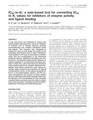
Figure 1. The Ligands tab of the Virtual Screening Workflow panel. 

Identifying Ligands and their States 

In the docking sequence, you can choose to keep all the ionization and tautomeric states of a 

given compound for which one of these states docks well. The ionization and tautomeric states 

that originate from the same compound are identified by their title. It is therefore necessary to 

set the title property. The controls under Create ligand titles to identify unique compounds by 

enable you to set or select the title for the ligands. The controls for setting the title are not 

available until you have specified the ligand files. 

8 



If the structures you have are all unique compounds, you can assign a unique title to each with 

the first option, Giving each structure a unique title. The title that is assigned is an integer. 

If the structures contain different ionization states or tautomers of the same compound, you can 

assign a title by selecting Using property and choosing a property from the option menu. The 

property names are taken from the first structure in each file, and only those properties that 

exist in each file are presented. You should ensure that the property you choose exists for each 

structure in the file, not just the first. The option menu becomes available when a file with valid 

properties is specified. 

When the title is set, a new property is created to store the original title. 

Preparing Ligands with LigPrep 

If your structures are already 3D all-atom structures with the appropriate ionization and tautomeric 

states, you do not need to prepare the ligands, and you can deselect the Prepare ligands 

option. Otherwise, ensure that this option is selected, and choose the desired options for generation 

of states for each ligand. 

You can choose to regularize the input geometries, so that ligands that are identical apart from 

small deviations in the atom positions are always treated the same. To do so, select Regularize 

input geometries. This process is run prior to LigPrep, and uses a conversion to unique 

SMILES to ensure the same atom numbering and geometry. All atom properties are lost when 

you perform this conversion, but entry properties, including the title, are retained. 

To generate ionization (protonation) states that are likely to exist in a given pH range, enter the 

target pH and the range in the Generate states at pH text boxes. You can generate these states 

with either the Ionizer or Epik, by selecting the appropriate option. Epik is licensed separately 

from LigPrep; the Ionizer is included with LigPrep. In addition to varying the ionization state, 

LigPrep generates tautomeric states that are likely in the given pH range. You can remove 

ionization and tautomeric states that have large penalties by selecting Remove high-energy 

ionization/tautomer states. These are states that are likely to have low populations at the 

prevailing conditions. If you select Epik for state generation, you can also generate extra states 

that are appropriate for binding to metals in metalloproteins, by selecting Add Epik metal 

binding states. These states are not normally generated at physiological pH. 

The LigPrep run varies the stereochemistry, if it is not predetermined. Any existing chirality 

information in the input file is preserved, and chemically reasonable chiralities are initially 

assigned for steroids, fused ring systems, and peptides. If you already have 3D structures, you 

can select 3D Geometry for Obtain stereochemical information from to determine the stereochemistry 

from the structure; otherwise select 2D parities to make use of information in 2D 

structure files. For the unspecified stereocenters, up to 32 stereoisomers are generated. These 

are ranked by energy, and only the lowest-energy stereoisomers are returned. You can control 



how many are returned by entering the number to return in the Unspecified stereocenters: 

retain up to N low-energy stereoisomers text box. 

Ring conformations are varied by LigPrep. You can limit the number of ring conformations 

returned by entering the maximum number in the Sample 5/6 membered rings: retain up to N 

conformations per ligand text box. This sampling does not include 7-membered and larger 

rings, which can be sampled with MacroModel after ligand preparation by selecting Enhance 

sampling of large rings using MacroModel. 

Filtering Ligands Prior to Docking 

The Virtual Screening Workflow offers three choices for prefiltering ligands: prefiltering using 

Lipinski’s Rule of 5, removing ligands with reactive functional groups, and prefiltering with a 

custom filter. Ligands that do not meet the specified criteria are removed from the ligand list 

for docking. Both prefiltering choices use ligfilter, which can filter the structures in a 

Maestro file based on any property in the file. 

Filtering by Lipinski’s Rule 

To prefilter the ligands using Lipinski’s Rule of 5, select Prefilter by Lipinski’s Rule. Ligands 

that do not satisfy this rule are not docked. This option requires QikProp properties. If the input 

structure files do not have QikProp properties, select Run QikProp. 

Filtering Out Reactive Functional Groups 

To filter out ligands that have reactive functional groups, select Remove ligands with reactive 

functional groups. The functional groups that are considered reactive are: 

• Acyl halides 

• Sulfonyl halides 

• Sulfinyl halides 

• Sulfenyl halides 

• Alkyl halides without 

fluorine 

• Anhydrides 

• Perhalomethylketones 

• Aldehydes 

• Formates 

• Peroxides 

• R-S-O-R 

• Isothiocyanates 

• Isocyanates 

• Phosphinyl halides 

• Phosphonyl halides 

• Alkali metals 

• Alkaline-earth metals 

• Lanthanide series metals 

• Actinide series metals 

• Transition metals 

• Other metals 

• Toxic nonmetals 

• Noble gases 

• Carbodiimides 

• Silyl enol ethers 

• Nitroalkanes 

• Phosphines 

• Alkyl sulfonates 

• Epoxides 

• Azides 

• Diazonium compounds 

• Isonitriles 

• Halopyrimidines 

• 1,2-Dicarbonyls 

• Michael acceptors 

• Beta-heterosubstituted 

carbonyls 

• Diazo compounds 

• R-N-S-R 

• Disulfides 

10 



Figure 2. The Filtering Options dialog box, showing the General Attributes tab. 

Filtering with Custom Filters 

To set up your own filter, select Retain only ligands matching criteria, then click Criteria to set 

up or read in the filter. The Filter options dialog box opens, which allows you to define the 

filtering criteria or read a file containing filtering criteria. 

Filters are constructed from a combination of criteria set for various Maestro properties, 

certain predefined feature counts, or counts of SMARTS patterns for functional groups. Each 

ligand must meet all of the criteria to pass through the filter. 

The criteria are set by selecting an item from the list in one of the tabs, selecting a relational 

operator, and setting a value, then clicking Add. The criterion is added to the list at the bottom 

of the panel. You can delete a criterion by selecting it and clicking Delete. When you have 

added all the desired criteria, click OK to accept the filter. 

To read a filter, click Read criteria file, and navigate to the desired file in the file chooser that 

opens. The file must have the extension .lff. When you click OK, the file is read and the 

criteria are listed in the Filtering definitions and criteria text area. You can then add criteria to 

the list, or delete criteria from the list. 



Figure 3. The Add definition dialog box 

In the Properties tab, all properties that are defined in the input files for each ligand are listed. 

You can display properties by family (this includes product families, such as QikProp) to limit 

the range of properties available, by choosing the family from the Show family option menu. 

In the Functional Group Counts tab, you can create a new pattern by clicking New and selecting 

or entering patterns in the Add definition dialog box. This dialog box provides tools for 

including or excluding patterns: ligands must match included patterns, but must not match 

excluded patterns. A complex pattern can thus be built up out of simple patterns. You can 

choose from the existing patterns, or enter your own SMARTS pattern either by typing it in the 

text box or by selecting atoms in the Workspace and clicking Get From Selection. Then click 

Include or Exclude to add the pattern to the definition. The pattern is added to the list in the 

lower half of the dialog box. You can delete patterns from this list by selecting them and 

clicking Delete. To view the definition of an existing pattern, select the pattern and click View 

definition. To complete the pattern definition, enter a name in the Name of new functional group 

text box at the top of the dialog box, and click Add. 

When you have finished setting up the filter, you can choose whether to apply the filter before 

preparing the ligands, or afterwards, by selecting Before preparation or After preparation. 

Filtering that depends only on 2D properties, such as functional group counts, can be done 

beforehand, and thus save the preparation time. Filtering that depends on 3D properties of the 

structures can only be done afterwards. 

12 



Setting Up the Receptors 

If you want to dock the ligands that you have prepared and filtered, you must specify one or 

more grids for the receptor. The ligands will be docked to each receptor that you specify. The 

tools for specifying the receptors are in the Receptors tab. This tab provides controls for 

selecting pregenerated grids, for generating grids from the Workspace structure, and for setting 

constraints. The grids are defined in the Receptor options section. They can then be added to 

the Receptors for docking table, by clicking Add. You can also edit the information for a grid 

and save it, or remove the grid from the table. 

Figure 4. The Receptors tab of the Virtual Screening Workflow panel. 



To add a receptor that has existing grids to the list: 

1. Select Use grids from file in the Receptor options section. 

2. Enter the path in the Grid text box, or click Browse and navigate to the grid. 

3. If you want to use constraints, click Constraints and make selections in the Constraints 

dialog box. 

4. Enter a name in the Identifier text box, to name the receptor. 

The default is to use a single letter. 

5. Enter a value in the GlideScore offset text box, if you want to shift the GlideScores for 

this receptor. 

6. Click Add. 

The receptor is added to the Receptors for docking table. 

To add a receptor that does not have existing grids to the list: 

1. Select Generate grids from Workspace in the Receptor options section. 

2. Display the receptor in the Workspace. 

If you want to use a ligand to define the grid, the receptor entry must include a ligand. If 

it does not, create a new entry by merging the receptor and the ligand entry. You cannot 

use multiple entries to define the grid. 

3. If the receptor entry contains a ligand, select Pick ligand to exclude and click on a ligand 

atom. 

4. Choose an option for defining the grid center: 

• Centroid of Workspace ligand—use the ligand centroid to define the grid center. 

• Centroid of selected residues—select the residues to define the grid center, by clicking 

Select and using the Atom Selection dialog box. 

• Supplied X, Y, Z coordinates—enter the coordinates of the grid center. 

5. Enter the maximum ligand size in the Dock ligands with length


8. If you want to use constraints, click Constraints and make selections in the Constraints 

dialog box. 

9. Enter a name in the Identifier text box, to name the receptor. 

The default is to use a numerical index. 

10. Enter a value in the GlideScore offset text box, if you want to shift the GlideScores for 

this receptor. 

11. Click Add. 

The receptor is added to the Receptors for docking table. 

Any receptor that you specify for grid generation must be properly prepared. To prepare a 

receptor, you can use the Protein Preparation Wizard panel, which you open from the Workflows 

menu. For information on protein preparation, see the Protein Preparation Guide. If the 

receptor has not been marked as prepared with the Protein Preparation Wizard, a warning 

dialog box opens when you start the job. This dialog box offers you the choice of marking the 

protein as prepared (if, for example, it was prepared with a previous software release), ignoring 

the indication that the protein is not prepared, or canceling. 

If you want to change any data associated with a receptor, click Edit. The receptor data is 

loaded into the Receptor options section, and you can make changes. When you have finished 

making changes, click Save. 

If you want to remove receptors from the table (and thus not use them), select the receptors and 

click Remove. The maximum number of receptors you can add is 100. 

Setting Constraints 

You can set up constraints for grids that are to be generated, you can request the use of 

constraints for both pregenerated and new grids, and you can set constraints on the ligand core 

position. All of these tasks are performed in the Constraints dialog box, which you open by 

clicking Constraints. Only H-bond and metal receptor constraints can be used, even if others 

are present, and only these constraints can be defined for a new grid. 

To set up a constraint for a new grid: 

1. Select Pick constraint atom. 

2. Pick the receptor atom for the constraint in the Workspace. 

The constraint is added to the table and marked in the Workspace. The type of constraint 

is determined from the type of the atom that you picked. 



Figure 5. The Constraints dialog box 

To request use of constraints in docking: 

1. Select the desired constraints in the Use column of the table. 

2. Select a Must match option. 

3. If you selected At least, enter the number of constraints that must be satisfied in the text 

box. 

To restrict the ligand core to a reference position: 

1. Select Restrict ligand core to reference position. 

2. Enter a tolerance for the RMSD of the ligand from the reference position in the Tolerance 

text box. 

3. Select Pick ligand for core constraint, and pick a ligand atom. 

You must have the receptor and ligand displayed to pick the ligand atom. 

4. Choose an option to define the core atoms in the ligand. 

The choices are All (all atoms in the ligand), All heavy (all nonhydrogen atoms in the 

ligand), and SMARTS. 

16 



5. If you chose SMARTS, enter the SMARTS pattern in the text box, or select the desired 

core atoms in the Workspace, and click Get from selection. 

6. If you want only the ligands that match the core pattern to be docked, select Skip ligands 

that do not match core pattern. 

When you have finished setting constraints, click OK. 

Setting Docking Options 

If you specified grids in the Receptors tab, you can choose which of the three docking accuracy 

levels to include and set various options for docking in the Docking Options tab. The 

docking options are described in detail in Chapter 5 of the Glide User Manual. 

Setting Common Options 

At the top of the Docking Options tab are several options that apply to all docking calculations. 

You can choose the force field from the Force Field option menu, from OPLS2001 and 

OPLS2005. The default is OPLS2001, because many of the parameters in the Glide program 

and the Glide scoring functions were optimized for OPLS_2001. Use of another force field— 

even one that is superior in other respects—can result in a degradation of the results. 

OPLS_2005 is offered as an alternative because it supports a wider range of atom types, 

including boron. 

If you want to minimize the poses after docking, select Perform post-docking minimizations. 

This can result in better poses. 

Glide can also add ionization and tautomerization penalties from Epik to the docking score, 

including those for metal binding if they were calculated. To include these penalties, select Use 

Epik penalties. 

Setting Ligand Scaling Parameters 

Below the common options is a section for scaling of ligand van der Waals radii. You can 

soften the nonpolar part of the ligand potential by scaling the van der Waals radii of ligand 

atoms with small partial charges. To do so, enter the scaling factor and the partial charge cutoff 

in the text boxes in the Scaling of ligand van der Waals radii section. See Section 5.3.4 of the 

Glide User Manual for more information. 



Figure 6. The Docking Options tab of the Virtual Screening Workflow panel. 

Setting Up the Docking Stages 

The lower part of the Docking Options tab allows you to choose which Glide docking runs to 

include in the workflow, and contains options for HTVS, SP, and XP docking runs. To include 

a docking run in the workflow, select the corresponding option. Under each option is a set of 

controls for the docking stage. A common set of controls is provided for each option, which 

are described below. In addition, there are mode-specific options, which are described after the 

common controls. 

18 



Common Controls 

There are two common options for the docking method for all stages: Dock flexibly and Dock 

rigidly. For SP and XP docking, two more options are available: Refine and Score in place. 

To apply constraints for the docking stage, select Use selected constraints for each grid. 

The Amide bonds option menu enables you to specify how to treat non-planar amide bonds. 

The options to choose from are: 

• Vary amide bond conformation—Allow non-planar conformations, without a particular 

penalty. 

• Allow trans conformers only—Only return results for conformations that are trans. 

• Retain original amide bond conformation—No variation of the conformation is permitted. 

• Penalize non-planar conformation—Apply a penalty to nonplanar amide bonds. 

The two Keep options allow you to specify the percentage (upper text box) or number (lower 

text box) of the best compounds to keep. A “compound” may consist of several ionization or 

tautomeric states, as generated by LigPrep. The option menu allows you to choose how many 

ionization or tautomeric states to keep for each compound. 

The options to choose from for HTVS and SP docking are: 

• All states (default for HTVS) 

• All good scoring states (default for SP) 

• Only best scoring states 

For XP docking, there are only two options: 

• All good scoring poses 

• Only best scoring pose (default) 

The rationale for keeping all ionization and tautomeric states is that the actual state that scores 

best can vary with the accuracy level. Keeping all states of a particular compound in the early 

stages ensures that the structures that will score best in later stages are not discarded. 

Specific Controls 

For XP docking there are several additional options: 

• Generate multiple input conformations—Run a MacroModel conformational search job 

on the input structures corresponding to the best poses from the previous stage to locate 

the lowest-energy conformer, using two different force fields. This option generates two 

extra input structures for XP docking, and therefore takes several times as long as an XP 



docking run with a single structure (including the conformational search). The variations 

in the input structures often produce better final results. 

• Write XP descriptor information—This option writes the descriptor information needed 

for the XP Visualizer, and requires a license for this feature. See Section 6.2 of the Glide 

User Manual for information on the XP Visualizer. 

• Compute maximum values by docking fragments—This option is only available if you 

select Write XP descriptor information. It performs an additional XP docking calculation 

of a set of 50 fragments that were chosen to maximize the various XP descriptors. These 

fragments can be used to gain insight into the nature of the binding energetics. You can 

view results for these fragments in the XP Visualizer, and use the results to evaluate how 

close the XP terms for ligands are to the maximum score. If you want to apply constraints 

to the fragments, select Apply constraints. 

• Generate N poses per compound state—This text box allows you to generate more than 

a single pose for each state. 

Postprocessing with Prime MM-GBSA 

At the end of any docking run, you can run a Prime MM-GBSA calculation on the final poses 

to obtain ligand binding energies, by selecting Postprocess with Prime MM-GBSA. This option 

requires a Prime license. 

Running Jobs 

When the general setup and the docking setup has been completed, click Start to open the Start 

dialog box, in which you can set job options and start the job. The run consists of a master (or 

“driver”) job and a set of subjobs. The master job starts all the subjobs for the various stages of 

the workflow, and collects the results. 

You can choose to run the master job on the local host by selecting Run master (driver) job on 

“localhost”, or you can run it on the selected host. The master job must have access to the input 

files and the current directory, but the host for the subjobs does not need access to these files 

and directory. 

Each stage of the workflow can be divided into a set of subjobs, which can be run concurrently. 

You can specify the number of subjobs in the Separate into N subjobs text box. You should 

consider all stages of the workflow when deciding on the number of subjobs. The master job 

may adjust the number of subjobs to better balance the load for each part of the workflow, so 

the number you enter is a target, not a requirement. If you are docking to more than one 

receptor, the workflow for each receptor can be distributed over multiple processors. 

20 



If you run multiple subjobs you can select a multiprocessor host such as a cluster from the 

Subjob host option menu. This host need not be the same as the master job host. You can also 

choose to limit the number of processors allocated to the subjobs by entering the maximum 

number in the Distribute subjobs over n processors text box. The number of processors should 

not be more than the number of subjobs. Otherwise, you can ensure that the maximum number 

of processors available is allocated to the execution of the subjobs by selecting Distribute 

subjobs over maximum available processors. 

Jobs can be monitored and controlled from the Maestro Monitor panel. 

You can also run jobs from the command line by clicking Write to write the input file, then 

running the following command: 

$SCHRODINGER/vsw [options] jobname.inp 

The options are listed in Table 1. The standard Job Control options, which are listed in 

Table 2.1 of the Job Control Guide, are supported. This includes the -HOST option, which is 

used to specify the hosts for the job. The –WAIT option, described in Table 2.2 of the Job 

Control Guide, is also supported. 

Table 1. Options for the vsw command. 

Option 

Description 

-NJOBS n 

Number of subjobs to generate without adjusting. If not specified, the number 

of subjobs is set to the number of processors and the -adjust option is 

set. 

-adjust Adjust the number of subjobs if the estimated job length is less than 10 

minutes or more than 20 hours. 

-host_ligprep hosts 

-host_glide hosts 

-host_prime hosts 

-host_mmod hosts 

-DRIVERHOST host 

-REMOTEDRIVER 

-LOCAL 

Run LigPrep jobs on the specified hosts. Default: run on hosts specified by 

–HOST. 

Run Glide jobs on the specified hosts. Default: run on hosts specified by 

–HOST. 

Run Prime jobs on the specified hosts. Default: run on hosts specified by 

–HOST. 

Run MacroModel jobs on the specified hosts. Default: run on hosts specified 

by –HOST. 

Run the driver job on the specified host. By default, the driver (master) job 

runs on the local host. 

Run the driver job on the first host in the list specified by -HOST. 

Run the driver job in local directory (default if the driver is run on the local 

host). 



Table 1. Options for the vsw command. (Continued) 

Option 

Description 

-NOLOCAL 

-RESTART 

-OVERWRITE 

-local 

-no_cleanup 

-max_retries n 

Restarting Jobs 

To restart a job, run it from the command line with the -RESTART option: 

$SCHRODINGER/vsw -RESTART [options] jobname.inp 

If you omit the -RESTART option, you will be prompted to indicate whether to resume the job 

where it left off, to restart it from the beginning, or to exit without doing anything. You can also 

reset the host and CPU information by setting the appropriate options. 

If you want to rerun a job and overwrite the output from the previous execution of the same 

job, use the -OVERWRITE option: 

$SCHRODINGER/vsw -OVERWRITE [options] jobname.inp 

Output Files 

Run the driver job in the scratch directory (default if he driver is run on a 

remote host). Jobs run with this option cannot be restarted. 

Restart the job. Restarting runs any subjobs that did not finish in the previous 

execution of the job. 

Overwrite any existing files when running the job. 

Do not create a temporary directory for each subjob. 

Do not remove intermediate files. 

Maximum number of times to restart subjobs if they fail. If not specified, 

the value specified by SCHRODINGER_MAX_RETRIES value is used, if 

defined, otherwise the default is 2. 

-v Display the version number and exit. 

-h[elp] 

Print usage message and exit. 

Output files are created in subdirectories of the working directory. The path to the output files 

is given at the end of the log file. For each receptor, a pose viewer file (_pv.mae) is created, 

containing the receptor and the docked ligands. In addition, the docked ligands are merged into 

a single file, with properties resulting from the merge, including the GlideScore offset, the 

receptor used, and the adjusted score. The merge is done by the glide_ensemble_merge 

utility, which is described below. The receptors are also placed in a single file. 

22 



Merging Results of Multiple Jobs 

Although you can include multiple receptors in a single run of the workflow, you may want to 

merge the results of several runs of the workflow into a single Glide pose viewer file. You can 

do this with the utility glide_ensemble_merge. In the process, you can specify a scoring 

offset for calibration of different runs. The results need not be from a single receptor: you can 

merge results for multiple receptors. The script combines sorted Glide pose viewer 

(*_pv.mae) files into an output file, sorted by default by GlideScore. 

The syntax is as follows: 

$SCHRODINGER/utilities/glide_ensemble_merge [options] 

job1_pv.mae[:offset1] job2_pv.mae[:offset2] 

[job3_pv.mae[:offset3] ... ] 

The options are listed in Table 2. The list of files to be merged is a blank-separated list of poseviewer 

file names. Each file name can be followed by a colon and an offset for the GlideScore. 

The default offset is zero. 

Table 2. Options for the glide_ensemble_merge utility. 

Option 

--version 

-h, --help 

-n maxlig, 

--nreport= maxlig 

-j jobname, 

--jobname= jobname 

-m mpl, 

-max_per_lig=mpl 

-f sortfield, 

--field=sortfield 

Description 

Display program version number and exit 

Display usage message and exit 

Maximum number of best ligands to keep after merging. Default: 10000. 

Job name. The output file is named jobname_pv.mae. Default name is 

glide_ensemble_merge. 

Maximum poses per ligand (default 1). Specify 0 (zero) to save all poses. 

Field (property value) by which the input files are sorted. Default is the GlideScore 

(r_i_glide_gscore). 

Citing the Virtual Screening Workflow in Publications 

Schrödinger Suite 2009 Virtual Screening Workflow; Glide version 5.5, Schrödinger, LLC, 

New York, NY, 2006; LigPrep version 2.3, Schrödinger, LLC, New York, NY, 2006; QikProp 

version 3.2, Schrödinger, LLC, New York, NY, 2006. 


24 



Getting Help 

Schrödinger software is distributed with documentation in PDF format. If the documentation is 

not installed in $SCHRODINGER/docs on a computer that you have access to, you should install 

it or ask your system administrator to install it. 

For help installing and setting up licenses for Schrödinger software and installing documentation, 

see the Installation Guide. For information on running jobs, see the Job Control Guide. 

Maestro has automatic, context-sensitive help (Auto-Help and Balloon Help, or tooltips), and 

an online help system. To get help, follow the steps below. 

• Check the Auto-Help text box, which is located at the foot of the main window. If help is 

available for the task you are performing, it is automatically displayed there. Auto-Help 

contains a single line of information. For more detailed information, use the online help. 

• If you want information about a GUI element, such as a button or option, there may be 

Balloon Help for the item. Pause the cursor over the element. If the Balloon Help does 

not appear, check that Show Balloon Help is selected in the Maestro menu of the main 

window. If there is Balloon Help for the element, it appears within a few seconds. 

• For information about a panel or the tab that is displayed in a panel, click the Help button 

in the panel, or press F1. The help topic is displayed in your browser. 

• For other information in the online help, open the default help topic by choosing Online 

Help from the Help menu on the main menu bar or by pressing CTRL+H. This topic is displayed 

in your browser. You can navigate to topics in the navigation bar. 

The Help menu also provides access to the manuals (including a full text search), the FAQ 

pages, the New Features pages, and several other topics. 

If you do not find the information you need in the Maestro help system, check the following 

sources: 

• Maestro User Manual, for detailed information on using Maestro 

• Maestro Command Reference Manual, for information on Maestro commands 

• Maestro Overview, for an overview of the main features of Maestro 

• Maestro Tutorial, for a tutorial introduction to basic Maestro features 

• Glide User Manual, for detailed information on using Glide 

• LigPrep User Manual, for detailed information on using LigPrep 

• QikProp User Manual, for detailed information on using QikProp 


Getting Help 

• Frequently Asked Questions pages, at 

https://www.schrodinger.com/VSW_FAQ.html 

• Known Issues pages, available on the Support Center. 

The manuals are also available in PDF format from the Schrödinger Support Center. Local 

copies of the FAQs and Known Issues pages can be viewed by opening the file 

Suite_2009_Index.html, which is in the docs directory of the software installation, and 

following the links to the relevant index pages. 

Information on available scripts can be found on the Script Center. Information on available 

software updates can be obtained by choosing Check for Updates from the Maestro menu. 

If you have questions that are not answered from any of the above sources, contact Schrödinger 

using the information below. 

E-mail: help@schrodinger.com 

USPS: Schrödinger, 101 SW Main Street, Suite 1300, Portland, OR 97204 

Phone: (503) 299-1150 

Fax: (503) 299-4532 

WWW: http://www.schrodinger.com 

FTP: ftp://ftp.schrodinger.com 

Generally, e-mail correspondence is best because you can send machine output, if necessary. 

When sending e-mail messages, please include the following information: 

• All relevant user input and machine output 

• Virtual Screening Workflow purchaser (company, research institution, or individual) 

• Primary Virtual Screening Workflow user 

• Computer platform type 

• Operating system with version number 

• Version numbers of products installed for Virtual Screening Workflow 

• Maestro version number 

• mmshare version number 

On UNIX you can obtain the machine and system information listed above by entering the 

following command at a shell prompt: 

$SCHRODINGER/utilities/postmortem 

This command generates a file named username-host-schrodinger.tar.gz, which you 

should send to help@schrodinger.com. If you have a job that failed, enter the following 

command: 

$SCHRODINGER/utilities/postmortem jobid 

26 


Getting Help 

where jobid is the job ID of the failed job, which you can find in the Monitor panel. This 

command archives job information as well as the machine and system information, and 

includes input and output files (but not structure files). If you have sensitive data in the job 

launch directory, you should move those files to another location first. The archive is named 

jobid-archive.tar.gz, and should be sent to help@schrodinger.com instead. 

If Maestro fails, an error report that contains the relevant information is written to the current 

working directory. The report is named maestro_error.txt, and should be sent to 

help@schrodinger.com. A message giving the location of this file is written to the terminal 

window. 

More information on the postmortem command can be found in Appendix A of the Job 

Control Guide. 

On Windows, machine and system information is stored on your desktop in the file 

schrodinger_machid.txt. If you have installed software versions for more than one 

release, there will be multiple copies of this file, named schrodinger_machid-N.txt, 

where N is a number. In this case you should check that you send the correct version of the file 

(which will usually be the latest version). 

If Maestro fails to start, send email to help@schrodinger.com describing the circumstances, 

and attach the file maestro_error.txt. If Maestro fails after startup, attach this file and the 

file maestro.EXE.dmp. These files can be found in the following directory: 

%USERPROFILE%\Local Settings\Application Data\Schrodinger\appcrash 


28 


120 West 45th Street, 29th Floor 

New York, NY 10036 

101 SW Main Street, Suite 1300 

Portland, OR 97204 

8910 University Center Lane, Suite 270 

San Diego, CA 92122 

Zeppelinstraße 13 

81669 München, Germany 

Dynamostraße 13 

68165 Mannheim, Germany 

Quatro House, Frimley Road 

Camberley GU16 7ER, United Kingdom 

SCHRÖDINGER ®

Virtual Screening Workflow - ISP

Create successful ePaper yourself

Delete template?

Save as template?