Chapter 8: Relaxation - The James Keeler Group

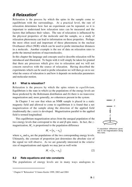
8 Relaxation †
Relaxation is the process by which the spins in the sample come to
equilibrium with the surroundings. At a practical level, the rate of
relaxation determines how fast an experiment can be repeated, so it is
important to understand how relaxation rates can be measured and the
factors that influence their values. The rate of relaxation is influenced by
the physical properties of the molecule and the sample, so a study of
relaxation phenomena can lead to information on these properties. Perhaps
the most often used and important of these phenomena in the nuclear
Overhauser effect (NOE) which can be used to probe internuclear distances
in a molecule. Another example is the use of data on relaxation rates to
probe the internal motions of macromolecules.
In this chapter the language and concepts used to describe relaxation will be
introduced and illustrated. To begin with it will simply be taken for granted
that there are processes which give rise to relaxation and we will not
concern ourselves with the source of relaxation. Having described the
experiments which can be used to probe relaxation we will then go on to see
what the source of relaxation is and how it depends on molecular parameters
and molecular motion.
8.1 What is relaxation
Relaxation is the process by which the spins return to equilibrium.
Equilibrium is the state in which (a) the populations of the energy levels are
those predicted by the Boltzmann distribution and (b) there is no transverse
magnetization and, more generally, no coherences present in the system.
In Chapter 3 we saw that when an NMR sample is placed in a static
magnetic field and allowed to come to equilibrium it is found that a net
magnetization of the sample along the direction of the applied field
(traditionally the z-axis) is developed. Magnetization parallel to the applied
field is termed longitudinal.
This equilibrium magnetization arises from the unequal population of the
two energy levels that correspond to the α and β spin states. In fact, the z-
magnetization, M z
, is proportional to the population difference
M n − n
z ∝
( α β )
where n α
and n β
are the populations of the two corresponding energy levels.
Ultimately, the constant of proportion just determines the absolute size of
the signal we will observe. As we are generally interested in the relative
size of magnetizations and signals we may just as well write
( )
M = z
n − α
nβ [2]
x
z
α
A population difference gives
rise to net magnetization along
the z-axis.
β
y
8.2 Rate equations and rate constants
The populations of energy levels are in many ways analogous to
†
Chapter 8 "Relaxation" © James Keeler 1999, 2002 and 2004
8–1

β
α
W
β
α
W
concentrations in chemical kinetics, and many of the same techniques that
are used to describe the rates of chemical reactions can also be used to
describe the dynamics of populations. This will lead to a description of the
dynamics of the z-magnetization.
Suppose that the populations of the α and β states at time t are n α
and n β
,
respectively. If these are not the equilibrium values, then for the system to
reach equilibrium the population of one level must increase and that of the
other must decrease. This implies that there must be transitions between the
two levels i.e. something must happen which causes a spin to move from the
α state to the β state or vice versa. It is this process which results in
relaxation.
The simplest assumption that we can make about the rate of transitions
from α to β is that it is proportional to the population of state α, n α
, and is a
first order process with rate constant W. With these assumptions the rate of
loss of population from state α is Wn α
. In the same way, the rate of loss of
population of state β is Wn β
.
However, the key thing to realize is that whereas a transition from α to β
causes a loss of population of level α, a transition from β to α causes the
population of state α to increase. So we can write
A transition from state α to
state β decreases the
population of state α , but a
transition from state β to state α
increases the population of
state α.
rate of change of population of state α = – Wn α
+ Wn β
The first term is negative as it represents a loss of population of state α and
in contrast the second term is positive as it represents a gain in the
population of state α. The rate of change of the population can be written
using the language of calculus as dn α
/dt so we have
dnα
=− Wnα
+ Wnβ
.
dt
Similarly we can write for the population of state β:
dnβ
=− Wnβ
+ Wnα
.
dt
These equations are almost correct, but we need to make one
modification. At equilibrium the populations are not changing so dn α
/dt =
0; this immediately implies that at equilibrium n α
= n β
, which simply is not
correct. We know that at equilibrium the population of state α exceeds that
of state β. This defect is easily remedied by replacing the population n α
0
with the deviation of the population from its equilibrium value ( nα
− nα)
,
where n 0 α
is the population of state α at equilibrium. Doing the same with
state β gives us the final, correct, equations:
dn
dn
α
β
= Wn ( β
−n 0 β)−Wn ( α
−n
0 α) = Wn ( α
−n 0 α)−Wn ( β
−n
0
β)
.
dt
dt
You will recognise here that this kind of approach is exactly the same as
that used to analyse the kinetics of a reversible chemical reaction.
Using Eqn. [2], we can use these two equations to work out how the z-
magnetization varies with time:
8–2

dM
dt
where M = n −n
z
( )
d nα
− nβ
=
dt
dn
dn
α β
= −
dt
dt
= Wn ( −n)−Wn ( −n)−Wn ( −n)+ Wn −n
0 0
=−2Wn ( α
−nβ )+ 2Wn ( α
−nβ
)
0
=−2WM−M
( )
0 0 0
z α β
( z z )
( )
0 0 0 0
β β α α α α β β
, the equilibrium z-magnetization.
8.2.1 Consequences of the rate equation
The discussion in the previous section led to a (differential) equation
describing the motion of the z-magnetization
() =− ()−
dMz
t
0
Rz( Mz t Mz
)
[7]
dt
where the rate constant, R z
= 2W and M z
has been written as a function of
time, M z
(t), to remind us that it may change.
What this equations says is that the rate of change of M z
is proportional to
the deviation of M z
from its equilibrium value, M 0 z
. If M z
= M 0 z
, that is the
system is at equilibrium, the right-hand side of Eqn. [7] is zero and hence so
is the rate of change of M z
: nothing happens. On the other hand, if M z
deviates from M 0 z
there will be a rate of change of M z
, and this rate will be
proportional to the deviation of M z
from M 0 z
. The change will also be such
as to return M z
to its equilibrium value, M 0 z
. In summary, Eqn. [7] predicts
that over time M z
will return to M 0 z
; this is exactly what we expect. The rate
at which this happens will depend on R z
.
This equation can easily be integrated:
dMz()
t
∫
Rzdt
( Mz()−
t Mz
) = −
0 ∫
0
ln( Mz()−
t Mz )=− Rt
z
+ const.
If, at time zero, the magnetization is M z
(0), the constant of integration can
0
be determined as ln( Mz( 0)−
Mz
). Hence, with some rearrangement:
or
ln M t M 0
⎡
z()−
⎤
z
⎢
Rt
z
⎣ Mz( )− M
⎥ =− 0
0
z ⎦
[ ] −
[7A]
0 0
Mz()= t Mz( 0)−
Mz exp ( Rt
z )+ Mz
[7B]
0
In words, this says that the z-magnetization returns from M z
(0) to M z
following an exponential law. The time constant of the exponential is 1/R z
,
and this is often called T 1
, the longitudinal or spin-lattice relaxation time.
8.2.2 The inversion recovery experiment
We described this experiment in section 3.10. First, a 180° pulse is applied,
8–3
M z
0
M z
M z (0)
t

thereby inverting the magnetization. Then a delay t is left for the
magnetization to relax. Finally, a 90° pulse is applied so that the size of the
z-magnetization can be measured.
S(t)–S
ln[ 0
–2S ] 0
Plot used to extract a value of
R z from the data from an
inversion recovery experiment.
t
We can now analyse this experiment fully. The starting condition for M z
0
is Mz( 0)=− Mz
, i.e. inversion. With this condition the predicted time
evolution can be found from Eqn. [7A] to be:
ln M t M 0
⎡
z()−
⎤
z
⎢
Rt
z
⎣ − M
⎥ =−
0
2
z ⎦
Recall that the amplitude of the signal we record in this experiment is
proportional to the z-magnetization. So, if this signal is S(t) it follows that
()−
⎡
ln⎢
St S
0
⎣ −2S
0
⎤
⎥
⎦
=−
Rt z
[7C]
where S 0 is the signal intensity from equilibrium magnetization; we would
find this from a simple 90° – acquire experiment.
Equation [7C] implies that a plot of ln[ ( St ()− S 0 ) −2 S
0
] against t should
be a straight line of slope –R z
. This, then, is the basis of a method of
determining the relaxation rate constant.
8.2.3 A quick estimate for R z
(or T 1
)
Often we want to obtain a quick estimate for the relaxation rate constant (or,
equivalently, the relaxation time). One way to do this is to do an inversion
recovery experiment but rather than varying t systematically we look for the
value of t which results in no signal i.e. a null. If the time when S(t) is zero
is t null
it follows immediately from Eqn. [7C] that:
ln
ln
⎡1
2
1
⎣⎢ ⎤ 2⎦ ⎥ =− Rt R = = tnull
z null
or
z
or T
tnull
ln 2
Probably the most useful relationship is the last, which is T 1
≈ 1.4 t null
.
This method is rather crude, but it good enough for estimating T 1
. Armed
with this estimate we can then, for example, decide on the time to leave
between transients (typically three to five times T 1
).
8.2.4 Writing relaxation in terms of operators
As we saw in Chapter 6, in quantum mechanics z-magnetization is
represented by the operator I z
. It is therefore common to write Eqn. [7] in
terms of operators rather then magnetizations, to give:
dIz() t =− Rz Iz ()−
0
( t Iz
)
[8]
dt
where I z
(t) represents the z-magnetization at time t and I 0
z
represents the
equilibrium z-magnetization. As it stands this last equation seems to imply
that the operators change with time, which is not what is meant. What are
changing are the populations of the energy levels and these in turn lead to
changes in the z-magnetization represented by the operator. We will use
this notation from now on.
8–4

8.3 Solomon equations
The idea of writing differential equations for the populations, and then
transcribing these into magnetizations, is a particularly convenient way of
describing relaxation, especially in more complex system. This will be
illustrated in this section.
Consider a sample consisting of molecules which contain two spins, I
and S; the spins are not coupled. As was seen in section 2.4, the two spins
have between them four energy levels, which can be labelled according to
the spin states of the two spins.
4
|ββ>
W I
(2)
4
|ββ>
W 2
W 0
W S
(2)
2
|αβ>
|βα>
3
2
|αβ>
|βα>
3
1
|αα>
W S
(1)
1
|αα>
W I
(1)
(a)
(b)
Diagram (a) shows the energy levels of a two spin system; the levels are labelled with the spin of I first
and the spin of S second. The dashed arrows indicate allowed transitions of the I spin, and the solid
arrows indicate allowed transitions of the S spin. Diagram (b) shows the relaxation induced transitions
which are possible amongst the same set of levels.
It turns out that in such a system it is possible to have relaxation induced
transitions between all possible pairs of energy levels, even those transitions
which are forbidden in normal spectroscopy; why this is so will be seen in
detail below. The rate constants for the two allowed I spin transitions will
be denoted W () 1
( 2
I
and W ) I
, and likewise for the spin S transitions. The rate
constant for the transition between the αα and ββ states is denoted W 2
, the
"2" indicating that it is a double quantum transition. Finally, the rate
constant for the transition between the αβ and βα states is denoted W 0
, the
"0" indicating that it is a zero quantum transition.
Just in the same was as was done in Section 8.2, rate equations can be
written for the flow of population from any of the levels. For example, for
level 1
dn1 () 1 () 1
() 1
() 1
=−WS n1
−WI n1 − Wn
2 1
+ WS n2
+ WI
n3 + Wn
2 4
dt
The negative terms are rates which lead to a loss of population of level 1
and the positive terms are ones that lead to a gain in its population. As was
discussed in section 8.2 the populations ought to be written as deviations
from their equilibrium values, ( ni
− n
0 i ). However, to do this results in
unnecessary complexity; rather, the calculation will be carried forward as
written and then at the last stage the populations will be replaced by their
deviations from equilibrium.
The corresponding equations for the other populations are
8–5

dn2 () 1
( 2) () 1 ( 2)
=−WS n2
−WI n2 − Wn
0 2
+ WS n1
+ WI
n4 + Wn
0 3
dt
dn3 () 1
( 2) () 1 ( 2)
=−WI n3
−WS n3 − Wn
0 3
+ WI n1
+ WS
n4 + Wn
0 2
dt
dn4 ( 2) ( 2)
( 2) ( 2)
=−WS
n4
−WI
n4 − Wn
2 4
+ WS
n3
+ WI
n2 + Wn
2 1
dt
All of this can be expressed in a more compact way if we introduce the I
and S spin z-magnetizations. The I spin magnetization is equal to the
population difference across the two I spin transitions, 1–3 and 2–4
I = n − z
n + n −
1 3 2
n4 [9]
As discussed above, the magnetization has been represented as the
corresponding operator, I z
. Likewise for the S-spin magnetization
S = n − z
n + n −
1 2 3
n4 [10]
A third combination of populations will be needed, which is represented by
the operator 2I z
S z
2IS = n − 1
n − z z 3
n + 2
n
[11]
4
Comparing this with Eq. [9] reveals that 2I z
S z
represents the difference in
population differences across the two I-spin transitions; likewise,
comparison with Eq. [10] shows that the same operator also represents the
difference in population differences across the two S-spin transitions.
Taking the derivative of Eq. [9] and then substituting for the derivatives
of the populations gives
dI z
dn1 dn3 dn2 dn4
= − + −
dt
dt
dt
dt
dt
() 1 () 1
() 1
() 1
=−W n −W n − Wn + W n + W n + Wn
8–6
S 1 I 1 2 1 S 2 I 3 2 4
() ( ) () ( )
4 0 2
1
2
1
2
+ WI n3
+ WS n3 + Wn
0 3
−WI n1
−WS
n −Wn
() 1
( 2) () 1 ( 2)
−W
n −W n − Wn + W n + W n + Wn
S 2 I 2 0 2 S 1 I 4 0 3
( 2) ( 2) ( 2) ( 2)
S 4 I 4 2 4 S 3 I 2 2 1
+ W n + W n + Wn −W n −W n −Wn
[12]
This unpromising looking equation can be expressed in terms of I z
, S z
etc. by
first introducing one more operator E, which is essentially the identity or
unit operator
E = n1 + n2 + n3 + n4 [13]
and then realizing that the populations, n i
, can be written in terms of E, I z
, S z
,
and 2I z
S z
:
1
n = E+ I + S + 2I S
1
4
1
n = E+ I −S −2I S
2
4
1
n = E− I + S −2I S
3
4
1
n = E− I − S + 2I S
4
4
( z z z z)
( z z z z)
( z z z z)
( )
z z z z
where these relationships can easily be verified by substituting back in the
definitions of the operators in terms of populations, Eqs. [9] – [13].
After some tedious algebra, the following differential equation is found

for I z
dIz
dt
() ( )
( I I 2 0)
1 2
=− W + W + W + W I
( ) − −
() ( )
z I I z z
1 2
− W −W S W W 2I S
2 0
z
( )
[14]
Similar algebra gives the following differential equations for the other
operators
dSz
() 1 ( 2) () 1 ( 2)
=−( W2 −W0) Iz − ( WS + WS + W2 + W0) Sz
−( WS −WS ) 2IzSz
dt
d2IS
z z
() 1 ( 2) () 1 ( 2)
=−( WI −WI ) Iz −( WS −WS
) Sz
dt
() 1 ( 2) () 1 ( )
− W + W + W + W
2
2I S
( I I S S ) z z
As expected, the total population, represented by E, does not change with
time. These three differential equations are known as the Solomon
equations.
It must be remembered that the populations used to derive these
equations are really the deviation of the populations from their equilibrium
values. As a result, the I and S spin magnetizations should properly be their
deviations from their equilibrium values, I 0
z
and S 0 z
; the equilibrium value
of 2I z
S z
is easily shown, from its definition, to be zero. For example, Eq.
[14] becomes
d
0
( z ) =−
() 1
WI +
( 2)
WI + W +
0
2
W0
Iz
Iz
Iz
− I
dt
( )( − )
( 2 0) − ( )
0 () 1 ( 2)
( z z )−
I
−
I
2
z z
− W −W S S W W I S
8.3.1 Interpreting the Solomon equations
What the Solomon equations predict is, for example, that the rate of change
of I z
depends not only on I z
− I 0 z
, but also on S z
− S 0 z
and 2I z
S z
. In other
words the way in which the magnetization on the I spin varies with time
depends on what is happening to the S spin – the two magnetizations are
connected. This phenomena, by which the magnetizations of the two
different spins are connected, is called cross relaxation.
The rate at which S magnetization is transferred to I magnetization is
given by the term
( )( − )
0
W 2
− W 0
Sz
S z
in Eq. [14]; (W 2
–W 0
) is called the cross-relaxation rate constant, and is
sometimes given the symbol σ IS
. It is clear that in the absence of the
relaxation pathways between the αα and ββ states (W 2
), or between the αβ
and βα states (W 0
), there will be no cross relaxation. This term is described
as giving rise to transfer from S to I as it says that the rate of change of the I
spin magnetization is proportional to the deviation of the S spin
magnetization from its equilibrium value. Thus, if the S spin is not at
equilibrium the I spin magnetization is perturbed.
In Eq. [14] the term
8–7

() 1 ( 2)
0
( WI + WI + W2 + W0) ( Iz
− Iz
)
describes the relaxation of I spin magnetization on its own; this is
sometimes called the self relaxation. Even if W 2
and W 0
are absent, self
relaxation still occurs. The self relaxation rate constant, given in the
previous equation as a sum of W values, is sometimes given the symbol R I
or ρ I
.
Finally, the term
( )
() ( )
I I z z
1 2
W − W 2I S
in Eq. [14] describes the transfer of I z
S z
into I spin magnetization. Recall
() 1
( 2)
that W I
and W I
are the relaxation induced rate constants for the two
allowed transitions of the I spin (1–3 and 2–4). Only if these two rate
constants are different will there be transfer from 2I z
S z
into I spin
magnetization. This situation arises when there is cross-correlation between
different relaxation mechanisms; a further discussion of this is beyond the
scope of these lectures. The rate constants for this transfer will be written
( ) = ( − )
() 1 ( 2) () 1 ( 2)
I I I S S S
∆ = W −W ∆ W W
According to the final Solomon equation, the operator 2I z
S z
shows self
relaxation with a rate constant
( )
() ( ) () ( )
IS I I S S
R = W + W + W + W
Note that the W 2
and W 0
pathways do not contribute to this. This rate
combined constant will be denoted R IS
.
Using these combined rate constants, the Solomon equations can be
written
I z
∆ I
σ IS
2I z S z
∆ S
S z
( ) =− −
0
d Iz
− Iz
0 0
RI( Iz
Iz )−σ
IS( Sz
−Sz )− ∆I2IzSz
dt
0
d( Sz
− Sz
) =−
IS
Iz
−
0 0
σ ( Iz )− RS ( Sz
−Sz )− ∆S2IzSz
[15]
dt
d2IS
z z
0 0
=−∆I( Iz
−Iz )−∆S( Sz
−Sz )− RIS2I z
S z
dt
The pathways between the different magnetization are visualized in the
0
diagram opposite. Note that as dIz
dt
= 0 (the equilibrium magnetization is
a constant), the derivatives on the left-hand side of these equations can
equally well be written dIz dt
and dSz dt.
It is important to realize that in such a system I z
and S z
do not relax with a
simple exponentials. They only do this if the differential equation is of the
form
dIz
0
=−RI( Iz −Iz
)
dt
which is plainly not the case here. For such a two-spin system, therefore, it
is not proper to talk of a "T 1
" relaxation time constant.
8–8

8.4 Nuclear Overhauser effect
The Solomon equations are an excellent way of understanding and
analysing experiments used to measure the nuclear Overhauser effect.
Before embarking on this discussion it is important to realize that although
the states represented by operators such as I z
and S z
cannot be observed
directly, they can be made observable by the application of a radiofrequency
pulse, ideally a 90° pulse
aI
z
( π 2)
I
x
⎯⎯⎯→−
aI
The subsequent recording of the free induction signal due to the evolution of
the operator I y
will give, after Fourier transformation, a spectrum with a
peak of size –a at frequency Ω I
. In effect, by computing the value of the
coefficient a, the appearance of the subsequently observed spectrum is
predicted.
The basis of the nuclear Overhauser effect can readily be seen from the
Solomon equation (for simplicity, it is assumed in this section that ∆ I
= ∆ S
=
0)
( ) =− −
0
d Iz
− Iz
0 0
RI ( Iz
Iz )−σ
IS( Sz
−Sz
)
dt
What this says is that if the S spin magnetization deviates from equilibrium
there will be a change in the I spin magnetization at a rate proportional to
(a) the cross-relaxation rate, σ IS
and (b) the extent of the deviation of the S
spin from equilibrium. This change in the I spin magnetization will
manifest itself as a change in the intensity in the corresponding spectrum,
and it is this change in intensity of the I spin when the S spin is perturbed
which is termed the nuclear Overhauser effect.
Plainly, there will be no such effect unless σ IS
is non-zero, which requires
the presence of the W 2
and W 0
relaxation pathways. It will be seen later on
that such pathways are only present when there is dipolar relaxation
between the two spins and that the resulting cross-relaxation rate constants
have a strong dependence on the distance between the two spins. The
observation of a nuclear Overhauser effect is therefore diagnostic of dipolar
relaxation and hence the proximity of pairs of spins. The effect is of
enormous value, therefore, in structure determination by NMR.
y
8–9

(a)
(b)
180°
S
τ m
90°
90°
Pulse sequence for recording
transient NOE enhancements.
Sequence (a) involves selective
inversion of the S spin – shown
here using a shaped pulse.
Sequence (b) is used to record
the reference spectrum in
which the intensities are
unperturbed.
8.4.1 Transient experiments
A simple experiment which reveals the NOE is to invert just the S spin by
applying a selective 180° pulse to its resonance. The S spin is then not at
equilibrium so magnetization is transferred to the I spin by cross-relaxation.
After a suitable period, called the mixing time, τ m
, a non-selective 90° pulse
is applied and the spectrum recorded.
After the selective pulse the situation is
( )= ( )=− [16]
0 0
Iz
0 Iz
Sz
0 Sz
where I z
has been written as I z
(t) to emphasize that it depends on time and
likewise for S. To work out what will happen during the mixing time the
differential equations
dIz() t =− RI Iz
()−
0 0
( t Iz )− σ
IS( Sz()−
t Sz
)
dt
dSz
() t =−
IS
Iz
()−
0 0
σ ( t Iz )− RS ( Sz()−
t Sz
)
dt
need to be solved (integrated) with this initial condition. One simple way to
do this is to use the initial rate approximation. This involves assuming that
the mixing time is sufficiently short that, on the right-hand side of the
equations, it can be assumed that the initial conditions set out in Eq. [16]
apply, so, for the first equation
dIz()
t
0 0 0 0
=−RI( Iz −Iz )−σ
IS( −Sz −Sz
)
dt
init
0
= 2σ
ISSz
This is now easy to integrate as the right-hand side has no dependence on
I z
(t)
τ
m
∫
0
0
dI t 2σ
S dt
z
()=
( )− ( )=
0
Iz τm Iz 0 2σISτmSz
I ( τ )= 2σ τ S + I
τ
m
∫
0
IS
0 0
z m IS m z z
This says that for zero mixing time the I magnetization is equal to its
equilibrium value, but that as the mixing time increases the I magnetization
has an additional contribution which is proportional to the mixing time and
the cross-relaxation rate, σ IS
. This latter term results in a change in the
intensity of the I spin signal, and this change is called an NOE enhancement.
z
8–10

The normal procedure for visualizing these enhancements is to record a
reference spectrum in which the intensities are unperturbed. In terms of z-
magnetizations this means that Iz,ref = I
0 z
. The difference spectrum, defined
as (perturbed spectrum – unperturbed spectrum) corresponds to the
difference
0 0 0
Iz( τm)− Iz, ref
= 2σISτmSz + Iz − Iz
0
= 2σ τ S
The NOE enhancement factor, η, is defined as
intensity in enhanced spectrum - intensity in reference spectrum
η =
intensity in reference spectrum
so in this case η is
z
τ
m ref σ τm
ητ ( m)= ( )− 0
I Iz,
2
IS
Sz
=
0
Iz,
ref
Iz
and if I and S are of the same nuclear species (e.g. both proton), their
equilibrium magnetizations are equal so that
ητ ( m)= 2σ IS
τm
Hence a plot of η against mixing time will give a straight line of slope σ IS
;
this is a method used for measuring the cross-relaxation rate constant. A
single experiment for one value of the mixing time will reveal the presence
of NOE enhancements.
This initial rate approximation is valid provided that
σISτm

These definitions ensure that λ 1
> λ 2
. If R I
and R S
are not too dissimilar, R is
of the order of σ IS
, and so the two rate constants λ 1
and λ 2
differ by a
quantity of the order of σ IS
.
As expected for these two coupled differential equations, integration
gives a time dependence which is the sum of two exponentials with different
time constants.
The figure below shows the typical behaviour predicted by these
equations (the parameters are R I
= R S
= 5σ IS
)
1.5
1.0
10 × (I z
–I z0
)/I z
0
(I z
/I z0
)
0.5
0
0.0
(S z
/I z0
)
time
-0.5
-1.0
The S spin magnetization returns to its equilibrium value with what appears
to be an exponential curve; in fact it is the sum of two exponentials but their
time constants are not sufficiently different for this to be discerned. The I
spin magnetization grows towards a maximum and then drops off back
towards the equilibrium value. The NOE enhancement is more easily
visualized by plotting the difference magnetization, (I z
– I 0 z
)/I 0 z
, on an
expanded scale; the plot now shows the positive NOE enhancement
reaching a maximum of about 15%.
Differentiation of the expression for I z
as a function of τ m
shows that the
maximum enhancement is reached at time
τ = 1 λ1
m,max
ln
λ1 − λ2
λ2
and that the maximum enhancement is
−λ1 −λ
Iz( τ I
R
R
m,max)−
z σ ⎛
IS
λ ⎞ λ
= ⎜ ⎟ − ⎛ 2
0 ⎡
⎤
2 ⎢
Iz
R ⎝ λ ⎠ ⎝ ⎜ ⎞
1
1 ⎥
0
⎢
⎟
λ ⎠ ⎥
2
2
⎣⎢
⎦⎥
8.4.2 The DPFGSE NOE experiment
From the point of view of the relaxation behaviour the DPFGSE experiment
is essentially identical to the transient NOE experiment. The only
difference is that the I spin starts out saturated rather than at equilibrium.
This does not influence the build up of the NOE enhancement on I. It does,
however, have the advantage of reducing the size of the I spin signal which
has to be removed in the difference experiment. Further discussion of this
experiment is deferred to Chapter 9.
8–12

8.4.3 Steady state experiments
The steady-state NOE experiment involves irradiating the S spin with a
radiofrequency field which is sufficiently weak that the I spin is not
affected. The irradiation is applied for long enough that the S spin is
saturated, meaning S z
= 0, and that the steady state has been reached, which
means that none of the magnetizations are changing, i.e. ( dIz
dt)= 0.
Under these conditions the first of Eqs. [15] can be written
therefore
d
0
( z )
Iz
− I
dt
SS
0 0
=−RI ( Iz,SS
−Iz )−σ
IS( 0−Sz
)= 0
σ 0 0
z
I
I = IS
R S + I
z,SS z
As in the transient experiment, the NOE enhancement is revealed by
subtracting a reference spectrum which has equilibrium intensities. The
NOE enhancement, as defined above, will be
0
Iz,SS
− Iz,
ref σ
IS
Sz
ηSS
= =
0
Iz,
ref
RI
Iz
In contrast to the transient experiment, the steady state enhancement only
depends on the relaxation of the receiving spin (here I); the relaxation rate
of the S spin does not enter into the relationship simply because this spin is
held saturated during the experiment.
It is important to realise that the value of the steady-state NOE
enhancement depends on the ratio of cross-relaxation rate constant to the
self relaxation rate constant for the spin which is receiving the enhancement.
If this spin is relaxing quickly, for example as a result of interaction with
many other spins, the size of the NOE enhancement will be reduced. So,
although the size of the enhancement does depend on the cross-relaxation
rate constant the size of the enhancement cannot be interpreted in terms of
this rate constant alone. This point is illustrated by the example in the
margin.
8.4.4 Advanced topic: NOESY
The dynamics of the NOE in NOESY are very similar to those for the
transient NOE experiment. The key difference is that instead of the
magnetization of the S spin being inverted at the start of the mixing time,
the magnetization has an amplitude label which depends on the evolution
during t l
.
Starting with equilibrium magnetization on the I and S spins, the z-
magnetizations present at the start of the mixing time are (other
magnetization will be rejected by appropriate phase cycling)
( )=− ( )=−
0
S 0 cosΩ
t1S I 0 cosΩ
t1I
The equation of motion for S z
is
0
z S z z I z
(a)
(b)
S
90°
90°
Pulse sequence for recording
steady state NOE
enhancements. Sequence (a)
involves selective irradiation of
the S spin leading to saturation.
Sequence (b) is used to record
the reference spectrum in
which the intensities are
unperturbed.
H B
H A
Y
H C
H D
X
Irradiation of proton B gives a
much larger enhancement on
proton A than on C despite the
fact that the distances to the
two spins are equal. The
smaller enhancement on C is
due to the fact that it is relaxing
more quickly than A, due to the
interaction with proton D.
t
t 2
1 τmix
Pulse sequence for NOESY.
8–13

() =− ()−
dSz
t
0 0
σ
IS( Iz
t Iz )− RS ( Sz()−
t Sz
)
dt
As before, the initial rate approximation will be used:
dSz( τ
m)
0 0
=−σ
( −cosΩ
tI
1
−I )− R −cosΩ
tS
1
−S
dt
init
0
0
= σ cosΩ
t + 1 I R cosΩ
t 1 S
( )
0 0
IS I z z S S z z
( ) + ( + )
IS I 1 z S S 1 z
Integrating gives
F 1
0
Ω I
{c}
{a}
{b}
F 2
Ω S
Ω S
Ω I
τ
m
∫
0
0
0
dS t σ cosΩ
t 1 I R cosΩ
t 1 S dt
z
τm
∫[ IS( I 1 ) z
+
S( S 1
+ ) z ]
0
()= +
( )− ( )= +
( ) + ( + )
0
0
Sz τm Sz 0 σISτm cosΩIt1
1 Iz RSτm
cosΩSt1
1 Sz
0
0
Sz( τm)= σISτm( cosΩIt1
+ 1)
Iz
+ Rτ
m( cosΩ
t1
+ 1) S − cosΩ
t1S
0 0
= σISτmIz + RSτmSz
{a}
0
cosΩ
t σ τ I
{b}
+
I 1[ IS m]
z
[ ]
+ cosΩ
t Rτ
−1
S
0
S 1 S m z
0
S S z S z
After the end of the mixing time, this z-magnetization on spin S is rendered
observable by the final 90° pulse; the magnetization is on spin S, and so will
precess at Ω S
during t 2
.
The three terms {a}, {b} and {c} all represent different peaks in the
NOESY spectrum.
Term {a} has no evolution as a function of t 1
and so will appear at F 1
= 0;
in t 2
it evolves at Ω S
. This is therefore an axial peak at {F 1
,F 2
} = {0, Ω S
}.
This peak arises from z-magnetization which has recovered during the
mixing time. In this initial rate limit, it is seen that the axial peak is zero for
zero mixing time and then grows linearly depending on R S
and σ IS
.
Term {b} evolves at Ω I
during t 1
and Ω S
during t 2
; it is therefore a cross
peak at {Ω I
, Ω S
}. The intensity of the cross peak grows linearly with the
mixing time and also depends on σ IS
; this is analogous to the transient NOE
experiment.
Term {c} evolves at Ω S
during t 1
and Ω S
during t 2
; it is therefore a
diagonal peak at {Ω S
, Ω S
} and as R s
τ m

8.4.5 Sign of the NOE enhancement
We see that the time dependence and size of the NOE enhancement depends
on the relative sizes of the cross-relaxation rate constant σ IS
and the self
relaxation rate constants R I
and R S
. It turns out that these self-rates are
always positive, but the cross-relaxation rate constant can be positive or
negative. The reason for this is that σ IS
= (W 2
– W 0
) and it is quite possible
for W 0
to be greater or less than W 2
.
A positive cross-relaxation rate constant means that if spin S deviates
from equilibrium cross-relaxation will increase the magnetization on spin I.
This leads to an increase in the signal from I, and hence a positive NOE
enhancement. This situation is typical for small molecules is non-viscous
solvents.
A negative cross-relaxation rate constant means that if spin S deviates
from equilibrium cross-relaxation will decrease the magnetization on spin I.
This leads to a negative NOE enhancement, a situation typical for large
molecules in viscous solvents. Under some conditions W 0
and W 2
can
become equal and then the NOE enhancement goes to zero.
8.5 Origins of relaxation
We now turn to the question as to what causes relaxation. Recall from
section 8.1 that relaxation involves transitions between energy levels, so
what we seek is the origin of these transitions. We already know from
Chapter 3 that transitions are caused by transverse magnetic fields (i.e. in
the xy-plane) which are oscillating close to the Larmor frequency. An RF
pulse gives rise to just such a field.
However, there is an important distinction between the kind of transitions
caused by RF pulses and those which lead to relaxation. When an RF pulse
is applied all of the spins experience the same oscillating field. The kind of
transitions which lead to relaxation are different in that the transverse fields
are local, meaning that they only affect a few spins and not the whole
sample. In addition, these fields vary randomly in direction and amplitude.
In fact, it is precisely their random nature which drives the sample to
equilibrium.
The fields which are responsible for relaxation are generated within the
sample, often due to interactions of spins with one another or with their
environment in some way. They are made time varying by the random
motions (rotations, in particular) which result from the thermal agitation of
the molecules and the collisions between them. Thus we will see that NMR
relaxation rate constants are particularly sensitive to molecular motion.
If the spins need to lose energy to return to equilibrium they give this up
to the motion of the molecules. Of course, the amounts of energy given up
by the spins are tiny compared to the kinetic energies that molecules have,
so they are hardly affected. Likewise, if the spins need to increase their
energy to go to equilibrium, for example if the population of the β state has
to be increased, this energy comes from the motion of the molecules.
Relaxation is essentially the process by which energy is allowed to flow
8–15

etween the spins and molecular motion. This is the origin of the original
name for longitudinal relaxation: spin-lattice relaxation. The lattice does
not refer to a solid, but to the motion of the molecules with which energy
can be exchanged.
8.5.1 Factors influencing the relaxation rate constant
The detailed theory of the calculation of relaxation rate constants is beyond
the scope of this course. However, we are in a position to discuss the kinds
of factors which influence these rate constants.
Let us consider the rate constant W ij
for transitions between levels i and j;
this turns out to depend on three factors:
We will consider each in turn.
W A Y J ω
= × × ( )
ij ij ij
The spin factor, A ij
This factor depends on the quantum mechanical details of the interaction.
For example, not all oscillating fields can cause transitions between all
levels. In a two spin system the transition between the αα and ββ cannot be
brought about by a simple oscillating field in the transverse plane; in fact it
needs a more complex interaction that is only present in the dipolar
mechanism (section 8.6.2). We can think of A ij
as representing a kind of
selection rule for the process – like a selection rule it may be zero for some
transitions.
The size factor, Y
This is just a measure of how large the interaction causing the relaxation is.
Its size depends on the detailed origin of the random fields and often it is
related to molecular geometry.
The spectral density, J(ω ij )
This is a measure of the amount of molecular motion which is at the correct
frequency, ω ij
, to cause the transitions. Recall that molecular motion is the
effect which makes the random fields vary with time. However, as we saw
with RF pulses, the field will only have an effect on the spins if it is
oscillating at the correct frequency. The spectral density is a measure of
how much of the motion is present at the correct frequency.
8.5.2 Spectral densities and correlation functions
The value of the spectral density, J(ω), has a large effect on relaxation rate
constants, so it is well worthwhile spending some time in understanding the
form that this function takes.
Correlation functions
8–16

To make the discussion concrete, suppose that a spin in a sample
experiences a magnetic field due to a dissolved paramagnetic species. The
size of the magnetic field will depend on the relative orientation of the spin
and the paramagnetic species, and as both are subject to random thermal
motion, this orientation will vary randomly with time (it is said to be a
random function of time), and so the magnetic field will be a random
function of time. Let the field experienced by this first spin be F 1
(t).
Now consider a second spin in the sample. This also experiences a
random magnetic field, F 2
(t), due to the interaction with the paramagnetic
species. At any instant, this random field will not be the same as that
experienced by the first spin.
For a macroscopic sample, each spin experiences a different random
field, F i
(t). There is no way that a detailed knowledge of each of these
random fields can be obtained, but in some cases it is possible to
characterise the overall behaviour of the system quite simply.
The average field experienced by the spins is found by taking the
ensemble average – that is adding up the fields for all members of the
ensemble (i.e. all spins in the system)
Ft ()= Ft
1()+ F2()+ t F3()+
t K
For random thermal motion, this ensemble average turns out to be
independent of the time; this is a property of stationary random functions.
Typically, the F i
(t) are signed quantities, randomly distributed about zero,
so this ensemble average will be zero.
An important property of random functions is the correlation function,
G(t,τ), defined as
* * *
G( t,
τ)= F() t F ( t + τ)+ F() t F ( t + τ)+ F() t F ( t + τ)+
1 1 2 2 3 3
K
( )
*
= FtF () t+
τ
F 1
(t) is the field experienced by spin 1 at time t, and F 1
(t+τ) is the field
experienced at a time τ later; the star indicates the complex conjugate,
which allows for the possibility that F(t) may be complex. If the time τ is
short the spins will not have moved very much and so F 1
(t+τ) will be very
*
little different from F 1
(t). As a result, the product FtF
1() 1 ( t+
τ ) will be
positive. This is illustrated in the figure below, plot (b).
(a) (b) (c)
F(t) F(t)F(t+1) F(t)F(t+15)
-1.2 5
-1.2 5
-1.2 5
(a) is a plot of the random function F(t) against time; there are about 100 separate time points. (b) is a
plot of the value of F multiplied by its value one data point later – i.e. one data point to the right; all
possible pairs are plotted. (c) is the same as (b) but for a time interval of 15 data points. The two
arrows indicate the spacing over which the correlation is calculated.
The same is true for all of the other members of then ensemble, so when the
*
FtF t τ are added together for a particular time, t, – that is, the
i
() ( + )
i
Paramagnetic species have
unpaired electrons. These
generate magnetic fields which
can interact with nearby nuclei.
On account of the large
gyromagnetic ratio of the
electron (when compared to the
nucleus) such paramagnetic
species are often a significant
source of relaxation.
a
b
c
d
Visualization of the different
timescales for random motion.
(a) is the starting position: the
black dots are spins and the
open circle represents a
paramagnetic species. (b) is a
snap shot a very short time
after (a); hardly any of the spins
have moved. (c) is a snapshot
at a longer time; more spins
have moved, but part of the
original pattern is still
discernible. (d) is after a long
time, all the spins have moved
and the original pattern is lost.
8–17

ensemble average is taken – the result will be for them to reinforce one
another and hence give a finite value for G(t,τ).
G( τ )
0
0
0
G(0)
τc
τ
As τ gets longer, the spin will have had more chance of moving and so
*
F 1
(t+τ) will differ more and more from F 1
(t); the product FtF
1() 1 ( t+
τ )
need not necessarily be positive. This is illustrated in plot (c) above. The
*
ensemble average of all these FtF
i() i ( t+
τ ) is thus less than it was when τ
was shorter. In the limit, once τ becomes sufficiently long, the
*
FtF
i() i ( t+
τ ) are randomly distributed and their ensemble average, G(t,τ),
goes to zero. G(t,τ) thus has its maximum value at τ = 0 and then decays to
zero at long times. For stationary random functions, the correlation function
is independent of the time t; it will therefore be written G(τ).
The correlation function, G(τ), is thus a function which characterises the
memory that the system has of a particular arrangement of spins in the
sample. For times τ which are much less than the time it takes for the
system to rearrange itself G(τ) will be close to its maximum value. As time
proceeds, the initial arrangement becomes more and more disturbed, and
G(τ) falls. For sufficiently long times, G(τ) tends to zero.
The simplest form for G(τ) is
( )
G( τ)= G( 0) exp − τ τc [18]
the variable τ appears as the modulus, resulting in the same value of G(τ)
for positive and negative values of τ. This means that the correlation is the
same with time τ before and time τ after the present time.
τ c
is called the correlation time. For times much less than the correlation
time the spins have not moved much and the correlation function is close to
its original value; when the time is of the order of τ c
significant
rearrangements have taken place and the correlation function has fallen to
about half its initial value. For times much longer than τ c
the spins have
moved to completely new positions and the correlation function has fallen
close to zero.
Spectral densities
The correlation function is a function of time, just like a free induction
decay. So, it can be Fourier transformed to give a function of frequency.
The resulting frequency domain function is called the spectral density; as
the name implies, the spectral density gives a measure of the amount of
motion present at different frequencies. The spectral density is usually
denoted J(ω)
Fourier Transform
G( τ)⎯ →J
ω
⎯⎯⎯⎯ ( )
8–18

If the spins were executing a well ordered motion, such as oscillating
back and forth about a mean position, the spectral density would show a
peak at that frequency. However, the spins are subject to random motions
with a range of different periods, so the spectral density shows a range of
frequencies rather than having peaks at discreet frequencies.
Generally, for random motion characterised by a correlation time τ c
,
frequencies from zero up to about 1/τ c
are present. The amount at
frequencies higher that 1/τ c
tails off quite rapidly as the frequency increases.
For a simple exponential correlation function, given in Eq. [18], the
corresponding spectral density is a Lorentzian
Fourier Transform 2τ
c
exp( −τ τc)⎯⎯⎯⎯⎯ → +
2 2
1 ωτc
This function is plotted in the margin; note how it drops off significantly
once the product ωτ c
begins to exceed ~1.
The plot opposite compares the spectral densities for three different
correlation times; curve a is the longest, b an intermediate value and c the
shortest. Note that as the correlation time decreases the spectral density
moves out to higher frequencies. However, the area under the plot remains
the same, so the contribution at lower frequencies is decreased. In
particular, at the frequency indicated by the dashed line the contribution at
correlation time b is greater than that for either correlation times a or c.
For this spectral density function, the maximum contribution at
frequency ω is found when τ c
is 1/ω; this has important consequences which
are described in the next section.
0
J( ω)
0 1 2 3 4 5
ωτ c
Plot of the spectral density as a
function of the dimensionless
variable ωτ c . The curve is a
lorentzian
J( ω)
a
b
c
0
ω
8.5.3 The "T 1
minimum"
In the case of relaxation of a single spin by a random field (such as that
generated by a paramagnetic species), the only relevant spectral density is
that at the Larmor frequency, ω 0
. This is hardly surprising as to cause
relaxation – that is to cause transitions – the field needs to have components
oscillating at the Larmor frequency.
We have just seen that for a given frequency, ω 0
, the spectral density is a
maximum when τ c
is 1/ω 0
, so to have the most rapid relaxation the
correlation time should be 1/ω 0
. This is illustrated in the plots below which
show the relaxation rate constant, W, and the corresponding relaxation time
(T 1
= 1/W) plotted as a function of the correlation time.
(a)
(b)
τ c
1/ω 0
τ c
W T 1
1/ω 0
Plot (a) shows how the relaxation rate constant, W, varies with the correlation time, τ c , for a given
Larmor frequency; there is a maximum in the rate constant when τ c = 1/ω 0 . Plot (b) shows the same
effect, but here we have plotted the relaxation time constant, T 1 ; this shows a minimum.
8–19

At very short correlation times (τ c
1. Clearly, which limit we are in depends on the Larmor frequency,
which in turn depends on the nucleus and the magnetic field.
For a Larmor frequency of 400 MHz we would expect the fastest
relaxation when the correlation time is 0.4 ns. Small molecules have
correlation times significantly shorter than this (say tens of ps), so such
molecules are clearly in the fast motion limit. Large molecules, such as
proteins, can easily have correlation times of the order of a few ns, and these
clearly fall in the slow motion limit.
Somewhat strangely, therefore, both very small and very large molecules
tend to relax more slowly than medium-sized molecules.
8.6 Relaxation mechanisms
So far, the source of the magnetic fields which give rise to relaxation and
the origin of their time dependence have not been considered. Each such
source is referred to as a relaxation mechanism. There are quite a range of
different mechanisms that can act, but of these only a few are really
important for spin half nuclei.
8.6.1 Paramagnetic species
We have already mentioned this source of varying fields several times. The
large magnetic moment of the electron means that paramagnetic species in
solution are particularly effective at promoting relaxation. Such species
include dissolved oxygen and certain transition metal compounds.
8.6.2 The dipolar mechanism
Each spin has associated with it a magnetic moment, and this is turn gives
rise to a magnetic field which can interact with other spins. Two spins are
thus required for this interaction, one to "create" the field and one to
"experience" it. However, their roles are reversible, in the sense that the
second spin creates a field which is experienced by the first. So, the overall
interaction is a property of the pair of nuclei.
8–20

The size of the interaction depends on the inverse cube of the distance
between the two nuclei and the direction of the vector joining the two
nuclei, measured relative to that of the applied magnetic field. As a
molecule tumbles in solution the direction of this vector changes and so the
magnetic field changes. Changes in the distance between the nuclei also
result in a change in the magnetic field. However, molecular vibrations,
which do give such changes, are generally at far too high frequencies to give
significant spectral density at the Larmor frequency. As a result, it is
generally changes in orientation which are responsible for relaxation.
The pair of interacting nuclei can be in the same or different molecules,
leading to intra- and inter-molecular relaxation. Generally, however, nuclei
in the same molecule can approach much more closely than those in
different molecules so that intra-molecular relaxation is dominant.
The relaxation induced by the dipolar coupling is proportional to the
square of the coupling. Thus it goes as
γ γ
1
2
1
2
2 6
r12
where γ 1
and γ 2
are the gyromagnetic ratios of the two nuclei involved and
r 12
is the distance between them.
As the size of the dipolar interaction depends on the product of the
gyromagnetic ratios of the two nuclei involved, and the resulting relaxation
rate constants depends on the square of this. Thus, pairs of nuclei with high
gyromagnetic ratios are most efficient at promoting relaxation. For
example, every thing else being equal, a proton-proton pair will relax 16
times faster than a carbon-13 proton pair.
It is important to realize that in dipolar relaxation the effect is not
primarily to distribute the energy from one of the spins to the other. This
would not, on its own, bring the spins to equilibrium. Rather, the dipolar
interaction provides a path by which energy can be transferred between the
lattice and the spins. In this case, the lattice is the molecular motion.
Essentially, the dipole-dipole interaction turns molecular motion into an
oscillating magnetic field which can cause transitions of the spins.
Relation to the NOE
The dipolar mechanism is the only common relaxation mechanism which
can cause transitions in which more than one spin flips. Specifically, with
reference to section 8.3, the dipolar mechanism gives rise to transitions
between the αα and ββ states (W 2
) and between the αβ and βα states (W 0
).
The rate constant W 2
corresponds to transitions which are at the sum of
the Larmor frequencies of the two spins, (ω 0,I
+ ω 0,S
) and so it is the spectral
density at this sum frequency which is relevant. In contrast, W 0
corresponds
to transitions at (ω 0,I
– ω 0,S
) and so for these it is the spectral density at this
difference frequency which is relevant.
In the case where the two spins are the same (e.g. two protons) the two
relevant spectral densities are J(2ω 0
) and J(0). In the fast motion limit (ω 0
τ c

calculation shows that W 2
> W 0
and so we expect to see positive NOE
enhancements (section 8.4.5). In contrast, in the slow motion limit (ω 0
τ c
>>
1) J(2ω 0
) is all but zero and so J(0) >> J(2ω 0
); not surprisingly it follows
that W 0
> W 2
and a negative NOE enhancement is seen.
8.6.3 The chemical shift anisotropy mechanism
The chemical shift arises because, due to the effect of the electrons in a
molecule, the magnetic field experienced by a nucleus is different to that
applied to the sample. In liquids, all that is observable is the average
chemical shift, which results from the molecule rapidly experiencing all
possible orientations by rapid molecular tumbling.
At a more detailed level, the magnetic field experienced by the nucleus
depends on the orientation of the molecule relative to the applied magnetic
field. This is called chemical shift anisotropy (CSA). In addition, it is not
only the magnitude of the field which is altered but also its direction. The
changes are very small, but sufficient to be detectable in the spectrum and to
give rise to relaxation.
One convenient way of imagining the effect of CSA is to say that due to
it there are small additional fields created at the nucleus – in general in all
three directions. These fields vary in size as the molecule reorients, and so
they have the necessary time variation to cause relaxation. As has already
been discussed, it is the transverse fields which will give rise to changes in
population.
The size of the CSA is specified by a tensor, which is a mathematical
object represented by a three by three matrix.
⎛σ σ σ ⎞
xx xy xz
σ = ⎜σ σ σ ⎟
yx yy yz
⎜
⎝σ σ σ ⎟
zx zy zz ⎠
The element σ xz
gives the size of the extra field in the x-direction which
results from a field being applied in the z-direction; likewise, σ yz
gives the
extra field in the y-direction and σ zz
that in the z-direction. These elements
depend on the electronic properties of the molecule and the orientation of
the molecule with respect to the magnetic field.
Detailed calculations show that the relaxation induced by CSA goes as
the square of the field strength and is also proportional to the shift
anisotropy. A rough estimate of the size of this anisotropy is that it is equal
to the typical shift range. So, CSA relaxation is expected to be significant
for nuclei with large shift ranges observed at high fields. It is usually
insignificant for protons.
8.7 Transverse relaxation
Right at the start of this section we mentioned that relaxation involved two
processes: the populations returning to equilibrium and the transverse
magnetization decaying to zero. So far, we have only discussed the fist of
these two. The second, in which the transverse magnetization decays, is
called transverse (or spin-spin) relaxation.
8–22

(a)
(b)
(c)
Depiction of how the individual contributions from different spins (shown on the left) add up to give the
net transverse magnetization (on the right). See text for details.
Each spin in the sample can be thought of as giving rise to a small
contribution to the magnetization; these contributions can be in any
direction, and in general have a component along x, y and z. The individual
contributions along z add up to give the net z-magnetization of the sample.
The transverse contributions behave in a more complex way as, just like
the net transverse magnetization, these contributions are precessing at the
Larmor frequency in the transverse plane. We can represent each of these
contributions by a vector precessing in the transverse plane.
The direction in which these vectors point can be specified by giving
each a phase – arbitrarily the angle measured around from the x-axis. It is
immediately clear that if these phases are random the net transverse
magnetization of the sample will be zero as all the individual contributions
will cancel. This is the situation that pertains at equilibrium and is shown in
(a) in the figure above.
For there to be net magnetization, the phases must not be random, rather
there has to be a preference for one direction; this is shown in (b) in the
figure above. In quantum mechanics this is described as a coherence. An
RF pulse applied to equilibrium magnetization generates transverse
magnetization, or in other words the pulse generates a coherence.
Transverse relaxation destroys this coherence by destroying the alignment
of the individual contributions, as shown in (c) above.
Our picture indicates that there are two ways in which the coherence
could be destroyed. The first is to make the vectors jump to new positions,
8–23

at random. Drawing on our analogy between these vectors and the
behaviour of the bulk magnetization, we can see that these jumps could be
brought about by local oscillating fields which have the same effect as
pulses.
This is exactly what causes longitudinal relaxation, in which we imagine
the local fields causing the spins to flip. So, anything that causes
longitudinal relaxation will also cause transverse relaxation.
The second way of destroying the coherence is to make the vectors get
out of step with one another as a result of them precessing at different
Larmor frequencies. Again, a local field plays the part we need but this
time we do not need it to oscillate; rather, all we need for it to do is to be
different at different locations in the sample.
This latter contribution is called the secular part of transverse relaxation;
the part which has the same origin as longitudinal relaxation is called the
non-secular part.
It turns out that the secular part depends on the spectral density at zero
frequency, J(0). We can see that this makes sense as this part of transverse
relaxation requires no transitions, just a field to cause a local variation in the
magnetic field. Looking at the result from section 8.5.2 we see that J(0) =
2τ c
, and so as the correlation time gets longer and longer, so too does the
relaxation rate constant. Thus large molecules in the slow motion limit are
characterised by very rapid transverse relaxation; this is in contrast to
longitudinal relaxation is most rapid for a particular value of the correlation
time.
The plot below compares the behaviour of the longitudinal and transverse
relaxation rate constants. As the correlation time increases the longitudinal
rate constant goes through a maximum. However, the transverse rate
constant carries on increasing and shows no such maximum. We can
attribute this to the secular part of transverse relaxation which depends on
J(0) and which simply goes on increasing as the correlation time increases.
Detailed calculations show that in the fast motion limit the two relaxation
rate constants are equal.
W
transverse
longitudinal
τ c
1/ω 0
Comparison of the longitudinal and transverse relaxation rate constants as a function of the correlation
time for the fixed Larmor frequency. The longitudinal rate constant shows a maximum, but the
transverse rate constant simply goes on increasing.
8–24