A spatially resolved study of ionized regions in galaxies at different ...
A spatially resolved study of ionized regions in galaxies at different ...
A spatially resolved study of ionized regions in galaxies at different ...

Create successful ePaper yourself
Turn your PDF publications into a flip-book with our unique Google optimized e-Paper software.
112 4 • Long-slit spectrophotometry <strong>of</strong> multiple knots <strong>of</strong> Hii <strong>galaxies</strong><br />
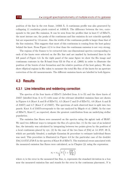
position <strong>of</strong> the l<strong>in</strong>e <strong>in</strong> the rest frame, λ 6563 Å. A cont<strong>in</strong>uum pr<strong>of</strong>ile was also gener<strong>at</strong>ed by<br />
collaps<strong>in</strong>g 11 resolution pixels centred <strong>at</strong> λ 6593 Å. The difference between the two, corresponds<br />
to the pure Hα emission. It can be seen from the pr<strong>of</strong>iles th<strong>at</strong> <strong>in</strong> knot C <strong>of</strong> IIZw71,<br />
the most <strong>in</strong>tense one, the peaks <strong>of</strong> the cont<strong>in</strong>uum and l<strong>in</strong>e emission do not co<strong>in</strong>cide <strong>sp<strong>at</strong>ially</strong><br />
but are separ<strong>at</strong>ed by 1.6 arcsec. Also the width <strong>of</strong> the cont<strong>in</strong>uum pr<strong>of</strong>ile is larger than th<strong>at</strong> <strong>of</strong><br />
the l<strong>in</strong>e emission. This suggests th<strong>at</strong> most <strong>of</strong> this cont<strong>in</strong>uum is com<strong>in</strong>g from the host galaxy<br />
beh<strong>in</strong>d the knot. From Figure 4.2 it is clear than the cont<strong>in</strong>uum emission is not very strong.<br />
The <strong>regions</strong> <strong>of</strong> the frames to be extracted <strong>in</strong>to one-dimensional spectra correspond<strong>in</strong>g to<br />
each <strong>of</strong> the knots were selected on the Hα l<strong>in</strong>e and are marked by horizontal l<strong>in</strong>es <strong>in</strong> the<br />
left panel <strong>of</strong> Figure 4.3. In the right panel <strong>of</strong> the same figure we show the Hα image and<br />
cont<strong>in</strong>uum contours <strong>in</strong> the R-band from Gil de Paz et al. (2003) <strong>in</strong> order to illustr<strong>at</strong>e the<br />
position <strong>of</strong> the bursts <strong>of</strong> star form<strong>at</strong>ion and the rel<strong>at</strong>ive position <strong>of</strong> the host galaxy. We also<br />
show elliptical <strong>regions</strong> <strong>in</strong> Hα taken to measure the total Hα flux <strong>of</strong> the knots for an aperture<br />
correction <strong>of</strong> the slit measurements. The <strong>different</strong> emission knots are labelled <strong>in</strong> both figures.<br />
4.3 Results<br />
4.3.1 L<strong>in</strong>e <strong>in</strong>tensities and redden<strong>in</strong>g correction<br />
The spectra <strong>of</strong> the four knots <strong>of</strong> IIZw71 (labelled from A to D) and the three knots <strong>of</strong><br />
J1657 (labelled from A to C) with some <strong>of</strong> the relevant identified emission l<strong>in</strong>es are shown<br />
<strong>in</strong> Figures 4.4 (Knot A and B <strong>of</strong> IIZw71), 4.5 (Knot C and D <strong>of</strong> IIZw71), 4.6 (Knot A and B<br />
<strong>of</strong> J1657) and 4.7 (Knot C <strong>of</strong> J1657). The spectrum <strong>of</strong> each observed knot is split <strong>in</strong>to two<br />
panels. Knot A <strong>of</strong> J1657corresponds to the one analyzed by Hägele et al. (2008). In the case<br />
<strong>of</strong> IIZw71, Knot C, as expected, shows the gre<strong>at</strong>est contribution from an underly<strong>in</strong>g stellar<br />
popul<strong>at</strong>ion.<br />
The emission l<strong>in</strong>e fluxes were measured on the spectra us<strong>in</strong>g the splot task <strong>of</strong> IRAF.<br />
We used two <strong>different</strong> ways to <strong>in</strong>tegr<strong>at</strong>e the flux <strong>of</strong> a given l<strong>in</strong>e. (1) In the case <strong>of</strong> an isol<strong>at</strong>ed<br />
l<strong>in</strong>e, the <strong>in</strong>tensity was calcul<strong>at</strong>ed by <strong>in</strong>tegr<strong>at</strong><strong>in</strong>g between two po<strong>in</strong>ts given by the position <strong>of</strong><br />
a local cont<strong>in</strong>uum placed by eye. (2) In the case <strong>of</strong> the two l<strong>in</strong>es <strong>of</strong> [Oii] <strong>at</strong> λλ 3727, 29 Å,<br />
which are partially blended, a multiple Gaussian fit procedure to estim<strong>at</strong>e <strong>in</strong>dividual fluxes<br />
was used. This procedure is illustr<strong>at</strong>ed <strong>in</strong> Figure 4.8 for the particular case <strong>of</strong> the doublet<br />
[Oii] λλ 3727,2729 Å <strong>in</strong> the spectra <strong>of</strong> Knot B <strong>of</strong> IIZw71. The st<strong>at</strong>istical errors associ<strong>at</strong>ed with<br />
the measured emission l<strong>in</strong>e fluxes were calcul<strong>at</strong>ed, as <strong>in</strong> Chapter §3, us<strong>in</strong>g the expression:<br />
σ l = σ c<br />
√N<br />
(<br />
1 + EW )<br />
N∆<br />
where σ l is the error <strong>in</strong> the measured l<strong>in</strong>e flux, σ c represents the standard devi<strong>at</strong>ion <strong>in</strong> a box<br />
near the measured emission l<strong>in</strong>e and stands for the error <strong>in</strong> the cont<strong>in</strong>uum placement, N is