A spatially resolved study of ionized regions in galaxies at different ...
A spatially resolved study of ionized regions in galaxies at different ...
A spatially resolved study of ionized regions in galaxies at different ...

You also want an ePaper? Increase the reach of your titles
YUMPU automatically turns print PDFs into web optimized ePapers that Google loves.
Facultad de Ciencias<br />
Departamento de<br />
Física Teórica<br />
Tesis Doctoral<br />
Universidad<br />
Autónoma<br />
de Madrid<br />
A<br />
<strong>sp<strong>at</strong>ially</strong> <strong>resolved</strong> <strong>study</strong><br />
<strong>of</strong><br />
<strong>ionized</strong> <strong>regions</strong> <strong>in</strong> <strong>galaxies</strong><br />
<strong>at</strong> <strong>different</strong> scales<br />
Rubén García Benito<br />
Rubén García Benito<br />
Directores:<br />
Ángeles I. Díaz Beltrán<br />
&<br />
Enrique Pérez Jiménez
Universidad Autónoma de Madrid<br />
Facultad de Ciencias<br />
Departamento de Física Teórica<br />
Grupo de Astr<strong>of</strong>ísica<br />
A <strong>sp<strong>at</strong>ially</strong> <strong>resolved</strong> <strong>study</strong> <strong>of</strong><br />
<strong>ionized</strong> <strong>regions</strong> <strong>in</strong> <strong>galaxies</strong><br />
<strong>at</strong> <strong>different</strong> scales<br />
Rubén García Benito<br />
Supervisors:<br />
Ángeles I. Díaz Beltrán<br />
&<br />
Enrique Pérez Jiménez<br />
A thesis submitted for the admission to the degree <strong>of</strong><br />
Doctor en Ciencias Físicas
A Abigaíl, mi ut<br />
A mi familia, por su apoyo
AGRADECIMIENTOS<br />
La trayectoria de una persona es la suma de las <strong>in</strong>fluencias de muchas otras en su vida.<br />
La mayoría de las veces son más los que no son recordados que los que una persona puede<br />
enumerar. Intentaré reflejar todas esas <strong>in</strong>fluencias en estas breves líneas.<br />
En primer lugar, tengo que agradecer mucho a mi directora de tesis, Ángeles. Lo primero<br />
es por darme la oportunidad de trabajar en el Observ<strong>at</strong>orio Astronómico de la Universidad<br />
Autónoma de Madrid, donde tuve mi primer contacto con el mundo de la astronomía observacional<br />
y pude disfrutar de “cacharrear” con telescopios, CCDs, filtros y demás cachivaches<br />
del observ<strong>at</strong>orio. Esta, s<strong>in</strong> duda, fue una etapa importante en mi formación <strong>in</strong>icial y gracias<br />
a ella pude aprender muchas cosas que de otro modo sólo hubieran formado parte de la experiencia<br />
a través del papel. En segundo lugar, y no por ello menos importante, por acogerme<br />
en su grupo de trabajo y por su confianza, tiempo, dedicación, y guía <strong>in</strong>cluso cuando me<br />
encontraba a 10000 kilómetros de distancia. S<strong>in</strong> ella, este trabajo no hubiera sido escrito.<br />
Otra persona que merece mi más s<strong>in</strong>cera gr<strong>at</strong>itud es mi codirector ES. Enrique. Gracias<br />
por confiar en mí y presentarme a NGC 5471. Gracias por acogerme repetidas veces en su<br />
despacho, por “pythonizarme”, por <strong>in</strong>f<strong>in</strong>idad de consejos, charlas sobre ciencia, divulgación,<br />
filos<strong>of</strong>ía, meditación y un s<strong>in</strong>fín de experiencias que han llenado la parte más humana del<br />
trabajo científico, el contacto con las personas. Muchas gracias, Enrique, he aprendido y<br />
disfrutado mucho contigo, y espero seguir haciéndolo.<br />
Otra persona que también es parte relevante en la creación de este trabajo y en mi<br />
formación es Enrique P. Montero. Un buen amigo que siempre ha estado ahí cuando lo<br />
necesitaba, me ha enseñado los secretos del cálculo de abundancias y de CLOUDY, me<br />
ha dado siempre su s<strong>in</strong>cera op<strong>in</strong>ión y ha compartido s<strong>in</strong> rechistar las habitaciones dobles<br />
cuando íbamos de congreso. Gracias por llevarme a observar al WHT, mi primera experiencia<br />
observacional. Espero que sigamos compartiendo trabajos científicos (y habitación).<br />
Tampoco quisiera olvidar a otras muchas personas que han aportado su granito de arena<br />
a estas pág<strong>in</strong>as, como Guillermo Hägele, Jesús Maíz, Miguel Cerviño, Pepe Vílchez (por<br />
su carta a Liu), Rosa González, Fabián Rosales, Elena y Roberto Terlevich, Jesús López,<br />
Sebastián Sánchez, Víctor Muñoz y tantos otros.
La gente del grupo de Astr<strong>of</strong>ísica ha compartido muchos momentos y, de una u otra<br />
manera, ha compartido conmigo sus conocimientos: Raúl, Alcione, Mónica (y Vale, por sus<br />
sonrisitas), Marta (que sigue s<strong>in</strong> perdonarme que me fuera del observ<strong>at</strong>orio), Jesús, Mariluz,<br />
José, Yago, Néstor, Jairo, Manuel, Carlos, Héctor, Alejandro, Marcelo y Alfredo.<br />
Mi estancia en Beij<strong>in</strong>g no hubiera sido la misma s<strong>in</strong> la fantástica acogida en el KIAA por<br />
Liu Xiaowei, Zhang N<strong>in</strong>g, Fang Xuan, Yuan Haibo, Bob Rub<strong>in</strong>, Herbert Lau, Huo Zhiy<strong>in</strong>g,<br />
Li Shul<strong>in</strong>, Pei Yu, Clement Baruteau, Douglas L<strong>in</strong>, Xiaoy<strong>in</strong> y muchos otros.<br />
De los amigos que han pasado por mi vida, s<strong>in</strong> lugar a dudas parte de mí no sería lo que<br />
es hoy s<strong>in</strong> la amistad de Alberto y Jorge, amigos con mayúsculas. A pesar de la distancia,<br />
siempre están presentes en mi corazón. También a Raúl, amigo de la <strong>in</strong>fancia, a Roberto y<br />
Ernesto, por su avidez por la ciencia, a Jaime, por sus aventuras, y a David y Francisco, por<br />
su amor por la música (¡aúpa el “Trío Castilla”!).<br />
Mi familia ha sido la fuerza <strong>in</strong>icial y origen de todo este trabajo. Gracias a mis padres,<br />
Begoña y Lorenzo, por darme la libertad de elegir mi cam<strong>in</strong>o, por la multitud de oportunidades<br />
que me han <strong>of</strong>recido, por su más que <strong>in</strong>f<strong>at</strong>igable apoyo, sacrificio y amor <strong>in</strong>condicional,<br />
por enseñarnos a mi hermana y a mí “la osa y el osito pequeño” en la terraza junto<br />
a una lámpara de queroseno, y por llevarnos a <strong>in</strong>f<strong>in</strong>idad de lugares. A mi hermana Nagore,<br />
por su confianza, su compañía (mi único “compañero” de universidad cuando estudiaba en<br />
la UNED) y porque siempre vela por mi salud, física o mental. Muchas gracias, familia.<br />
Y por último, a la persona que me ha acompañado realmente en este viaje de pr<strong>in</strong>cipio a<br />
f<strong>in</strong>, a la que he quitado más tiempo del que me hubiera gustado, la que me ha apoyado en todo<br />
momento, la que ha llenado de <strong>in</strong>strumentos y música mi vida. Gracias por acompañarme a<br />
lugares muy muy lejanos, por la paciencia que ha mostrado en todo momento (sobre todo con<br />
la maquetación del trabajo . . .), y por un s<strong>in</strong>fín de cosas de las que sólo ella es capaz. Gracias<br />
por su valor (¡ese día al volver de Tabarca!), pues ella es la que ha apostado verdaderamente<br />
por mí. Gracias por todo, Abi.
ABSTRACT<br />
In this thesis we have studied star form<strong>at</strong>ion processes <strong>in</strong> <strong>galaxies</strong> <strong>at</strong><br />
<strong>different</strong> scales: giant Hii <strong>regions</strong> <strong>in</strong> spiral discs and <strong>in</strong>dividual starburst<br />
knots <strong>in</strong> Hii <strong>galaxies</strong>.<br />
The first has revealed th<strong>at</strong> star form<strong>at</strong>ion <strong>in</strong> these <strong>regions</strong> is complex<br />
and, <strong>at</strong> least <strong>in</strong> NGC 5471, has proceeded <strong>in</strong> a general sp<strong>at</strong>io-temporal<br />
sequence from the halo <strong>in</strong>wards to the core. A remarkable abundance<br />
uniformity is found confirm<strong>in</strong>g previous results from classical works and<br />
valid<strong>at</strong><strong>in</strong>g the use <strong>of</strong> <strong>in</strong>tegr<strong>at</strong>ed spectroscopy to obta<strong>in</strong> abundances <strong>in</strong><br />
distant objects.<br />
The second has allowed a detailed abundance analysis <strong>of</strong> several<br />
star form<strong>in</strong>g knots <strong>in</strong> two Hii <strong>galaxies</strong> which shows no conclusive sp<strong>at</strong>ial<br />
vari<strong>at</strong>ions <strong>of</strong> the total abundances. S<strong>in</strong>ce there are stellar popul<strong>at</strong>ions<br />
old enough as to have produced supernovae, this implies either a very<br />
fast and effective mix<strong>in</strong>g with the surround<strong>in</strong>gs or th<strong>at</strong> the metals whose<br />
abundances are <strong>in</strong>ferred proceed from previous star form<strong>at</strong>ion events.<br />
RESUMEN<br />
En esta tesis presentamos un estudio de los procesos de formación<br />
estelar en galaxias a dos escalas diferentes: regiones Hii gigantes en<br />
discos de espirales y brotes <strong>in</strong>dividuales en galaxias Hii.<br />
La primera parte ha mostrado que la formación estelar en ese tipo<br />
de regiones es compleja y, al menos en NGC 5471, ha procedido en<br />
una secuencia general espacio-temporal desde el halo hacia el núcleo.<br />
También se ha hallado una abundancia uniforme confirmando resultados<br />
anteriores de trabajos clásicos, validando el uso de la espectroscopía<br />
<strong>in</strong>tegrada para obtener abundancias en objetos más distantes.<br />
En la segunda parte se ha llevado a cabo un análisis detallado de<br />
varios nodos de formación estelar en dos galaxias Hii. De los resultados<br />
no se concluye que haya variaciones espaciales de las abundancias<br />
totales. Ya que se encuentran poblaciones lo suficientemente<br />
viejas como para producir supernovas, esto implica que, o se produce<br />
un mezclado rápido y efectivo con el entorno, o los metales de los que<br />
se derivan las abundancias proceden de episodios anteriores de formación<br />
estelar.
Contents<br />
List <strong>of</strong> Figures<br />
List <strong>of</strong> Tables<br />
v<br />
ix<br />
1 • Introduction 1<br />
1.1 Overview . . . . . . . . . . . . . . . . . . . . . . . . . . . . . . . . . . . . . . 1<br />
1.1.1 Giant Extragalactic Hii <strong>regions</strong> . . . . . . . . . . . . . . . . . . . . . . 2<br />
1.1.2 Hii Galaxies . . . . . . . . . . . . . . . . . . . . . . . . . . . . . . . . 5<br />
1.2 Aims and structure <strong>of</strong> this work . . . . . . . . . . . . . . . . . . . . . . . . . . 8<br />
2 • The star form<strong>at</strong>ion history <strong>of</strong> NGC 5471 from cluster and <strong>resolved</strong><br />
stellar photometry 11<br />
2.1 Introduction . . . . . . . . . . . . . . . . . . . . . . . . . . . . . . . . . . . . . 11<br />
2.2 Observ<strong>at</strong>ions and D<strong>at</strong>a Reduction . . . . . . . . . . . . . . . . . . . . . . . . 13<br />
2.2.1 GALEX d<strong>at</strong>a . . . . . . . . . . . . . . . . . . . . . . . . . . . . . . . . 13<br />
2.2.2 HST/WFPC2 Imag<strong>in</strong>g . . . . . . . . . . . . . . . . . . . . . . . . . . . 14<br />
2.2.3 Near-<strong>in</strong>frared photometry . . . . . . . . . . . . . . . . . . . . . . . . . 17<br />
2.3 Results . . . . . . . . . . . . . . . . . . . . . . . . . . . . . . . . . . . . . . . 19<br />
2.3.1 Cluster Photometry . . . . . . . . . . . . . . . . . . . . . . . . . . . . 19<br />
2.3.2 Resolved Stellar Photometry . . . . . . . . . . . . . . . . . . . . . . . 24<br />
2.4 Discussion . . . . . . . . . . . . . . . . . . . . . . . . . . . . . . . . . . . . . 29<br />
2.4.1 Cluster Analysis . . . . . . . . . . . . . . . . . . . . . . . . . . . . . . 30<br />
2.4.2 CMD . . . . . . . . . . . . . . . . . . . . . . . . . . . . . . . . . . . . . 33<br />
3 • Integral Field Spectroscopy <strong>of</strong> Hii region complexes. The outer<br />
disk <strong>of</strong> NGC 6946 39<br />
3.1 Introduction . . . . . . . . . . . . . . . . . . . . . . . . . . . . . . . . . . . . . 39<br />
3.2 Observ<strong>at</strong>ions . . . . . . . . . . . . . . . . . . . . . . . . . . . . . . . . . . . . 42<br />
3.3 D<strong>at</strong>a Reduction . . . . . . . . . . . . . . . . . . . . . . . . . . . . . . . . . . . 44<br />
3.3.1 Pre-reduction . . . . . . . . . . . . . . . . . . . . . . . . . . . . . . . . 46<br />
i
ii<br />
CONTENTS<br />
3.3.2 Identific<strong>at</strong>ion <strong>of</strong> the position <strong>of</strong> the spectra . . . . . . . . . . . . . . . . 47<br />
3.3.3 Spectra extraction . . . . . . . . . . . . . . . . . . . . . . . . . . . . . 48<br />
3.3.4 Wavelength solution (dispersion correction) . . . . . . . . . . . . . . . 50<br />
3.3.5 Fiber-to-fiber response correction . . . . . . . . . . . . . . . . . . . . 51<br />
3.3.6 Flux-calibr<strong>at</strong>ion . . . . . . . . . . . . . . . . . . . . . . . . . . . . . . . 52<br />
3.3.7 Sky-subtraction . . . . . . . . . . . . . . . . . . . . . . . . . . . . . . . 57<br />
3.3.8 Mosaics . . . . . . . . . . . . . . . . . . . . . . . . . . . . . . . . . . . 58<br />
3.3.9 Correction for <strong>at</strong>mospheric absorption . . . . . . . . . . . . . . . . . . 59<br />
3.3.10 Correction for <strong>different</strong>ial <strong>at</strong>mospheric refraction . . . . . . . . . . . . 61<br />
3.4 Results . . . . . . . . . . . . . . . . . . . . . . . . . . . . . . . . . . . . . . . 63<br />
3.4.1 Subtraction <strong>of</strong> the underly<strong>in</strong>g popul<strong>at</strong>ion . . . . . . . . . . . . . . . . . 63<br />
3.4.2 L<strong>in</strong>e <strong>in</strong>tensities . . . . . . . . . . . . . . . . . . . . . . . . . . . . . . . 66<br />
3.4.3 Hα maps and morphology . . . . . . . . . . . . . . . . . . . . . . . . . 68<br />
3.4.4 Redden<strong>in</strong>g correction and c(Hβ) map . . . . . . . . . . . . . . . . . . 72<br />
3.4.5 Electron density . . . . . . . . . . . . . . . . . . . . . . . . . . . . . . 74<br />
3.4.6 Ioniz<strong>at</strong>ion structure and excit<strong>at</strong>ion . . . . . . . . . . . . . . . . . . . . 75<br />
3.4.7 Wolf-Rayet stellar popul<strong>at</strong>ion . . . . . . . . . . . . . . . . . . . . . . . 78<br />
3.4.8 Physical properties and chemical abundances from the <strong>in</strong>tegr<strong>at</strong>ed<br />
spectra . . . . . . . . . . . . . . . . . . . . . . . . . . . . . . . . . . . 81<br />
3.5 Discussion . . . . . . . . . . . . . . . . . . . . . . . . . . . . . . . . . . . . . 92<br />
3.5.1 Mass <strong>of</strong> the <strong>ionized</strong> gas . . . . . . . . . . . . . . . . . . . . . . . . . . 92<br />
3.5.2 Derived properties <strong>of</strong> the WR popul<strong>at</strong>ion . . . . . . . . . . . . . . . . 94<br />
3.5.3 Metal content . . . . . . . . . . . . . . . . . . . . . . . . . . . . . . . . 96<br />
3.5.4 Ioniz<strong>at</strong>ion structure . . . . . . . . . . . . . . . . . . . . . . . . . . . . . 99<br />
4 • Long-slit spectrophotometry <strong>of</strong> multiple knots <strong>of</strong> Hii <strong>galaxies</strong> 105<br />
4.1 Introduction . . . . . . . . . . . . . . . . . . . . . . . . . . . . . . . . . . . . . 105<br />
4.2 Observ<strong>at</strong>ions and reduction . . . . . . . . . . . . . . . . . . . . . . . . . . . . 107<br />
4.2.1 CAHA observ<strong>at</strong>ions . . . . . . . . . . . . . . . . . . . . . . . . . . . . 107<br />
4.2.2 WHT observ<strong>at</strong>ions . . . . . . . . . . . . . . . . . . . . . . . . . . . . . 108<br />
4.2.3 D<strong>at</strong>a reduction . . . . . . . . . . . . . . . . . . . . . . . . . . . . . . . 109<br />
4.3 Results . . . . . . . . . . . . . . . . . . . . . . . . . . . . . . . . . . . . . . . 112<br />
4.3.1 L<strong>in</strong>e <strong>in</strong>tensities and redden<strong>in</strong>g correction . . . . . . . . . . . . . . . . 112<br />
4.3.2 Physical conditions <strong>of</strong> the gas . . . . . . . . . . . . . . . . . . . . . . . 121<br />
4.3.3 Chemical abundance deriv<strong>at</strong>ion . . . . . . . . . . . . . . . . . . . . . 127<br />
4.4 Discussion . . . . . . . . . . . . . . . . . . . . . . . . . . . . . . . . . . . . . 131<br />
4.4.1 Gaseous physical conditions and element abundances . . . . . . . . 131<br />
4.4.2 Chemical abundances from empirical calibr<strong>at</strong>ors for Knots A and D <strong>of</strong><br />
IIZw71 . . . . . . . . . . . . . . . . . . . . . . . . . . . . . . . . . . . . 136<br />
4.4.3 The stellar popul<strong>at</strong>ion . . . . . . . . . . . . . . . . . . . . . . . . . . . 142<br />
4.4.4 Ionis<strong>in</strong>g stellar popul<strong>at</strong>ions . . . . . . . . . . . . . . . . . . . . . . . . 146<br />
4.4.5 K<strong>in</strong>em<strong>at</strong>ics and dynamics <strong>of</strong> the polar r<strong>in</strong>g . . . . . . . . . . . . . . . . 147<br />
5 • Conclusions and future work 149<br />
A •Interstellar Redden<strong>in</strong>g Corrections 159
CONTENTS<br />
iii<br />
B •Physical conditions <strong>of</strong> the gas and abundances 161<br />
B.1 Physical conditions <strong>of</strong> the gas . . . . . . . . . . . . . . . . . . . . . . . . . . . 161<br />
B.1.1 Density . . . . . . . . . . . . . . . . . . . . . . . . . . . . . . . . . . . 161<br />
B.1.2 Temper<strong>at</strong>ure . . . . . . . . . . . . . . . . . . . . . . . . . . . . . . . . 163<br />
B.2 Ionic abundances . . . . . . . . . . . . . . . . . . . . . . . . . . . . . . . . . . 164<br />
C •Empirical calibr<strong>at</strong>ors 169<br />
D •Stellar photometry results <strong>of</strong> NGC 5471 173<br />
References 189
List <strong>of</strong> Figures<br />
1.1 Sample <strong>of</strong> <strong>different</strong> scale and morphology Hii <strong>regions</strong> . . . . . . . . . . . . . 3<br />
1.2 Comparison <strong>of</strong> morphology <strong>of</strong> a GEHR and a BCD . . . . . . . . . . . . . . . 6<br />
1.3 Color-magnitude diagram <strong>of</strong> IZw18 . . . . . . . . . . . . . . . . . . . . . . . . 7<br />
2.1 Large scale image <strong>of</strong> M101 . . . . . . . . . . . . . . . . . . . . . . . . . . . . 12<br />
2.2 HST WFPC2 images <strong>of</strong> NGC 5471 . . . . . . . . . . . . . . . . . . . . . . . . 15<br />
2.3 Color composite <strong>of</strong> HST WFPC2 images <strong>of</strong> NGC 5471 . . . . . . . . . . . . . 16<br />
2.4 JHK s grayscale images and contour plots <strong>of</strong> NGC 5471 . . . . . . . . . . . . 18<br />
2.5 Plot <strong>of</strong> the def<strong>in</strong>ed eleven polygons . . . . . . . . . . . . . . . . . . . . . . . . 20<br />
2.6 Circular aperture <strong>of</strong> 15 ′′ overplotted on the Hα image . . . . . . . . . . . . . 22<br />
2.7 Decontam<strong>in</strong><strong>at</strong>ion <strong>of</strong> the NGC 5471 observed CMD . . . . . . . . . . . . . . . 27<br />
2.8 F<strong>in</strong>al CMD <strong>of</strong> NGC 5471 with isochrones . . . . . . . . . . . . . . . . . . . . 29<br />
2.9 Hα and J-V versus J-H plot . . . . . . . . . . . . . . . . . . . . . . . . . . . . 31<br />
2.10 F<strong>in</strong>al CMD with isochrones divided <strong>in</strong> b<strong>in</strong>s and lum<strong>in</strong>osity function . . . . . . 34<br />
2.11 Sp<strong>at</strong>ial distribution <strong>of</strong> the star form<strong>at</strong>ion with time . . . . . . . . . . . . . . . . 37<br />
3.1 Color composition image <strong>of</strong> NGC 6946 . . . . . . . . . . . . . . . . . . . . . 41<br />
3.2 Layout and dimensions <strong>of</strong> the PPak IFU . . . . . . . . . . . . . . . . . . . . . 43<br />
3.3 Hα image <strong>of</strong> NGC 6946 show<strong>in</strong>g the position <strong>of</strong> the PPak field . . . . . . . . 45<br />
3.4 Section <strong>of</strong> a PPak raw d<strong>at</strong>a . . . . . . . . . . . . . . . . . . . . . . . . . . . . 47<br />
3.5 Comparison <strong>of</strong> methods for the aperture extraction reduction step . . . . . . 48<br />
3.6 Left panel: Example <strong>of</strong> distortion along the cross-dispersion axis. Right panel:<br />
Example <strong>of</strong> shifts produces by a bad second order correction . . . . . . . . . 49<br />
3.7 Example <strong>of</strong> sky l<strong>in</strong>es used <strong>in</strong> the red spectra to f<strong>in</strong>d the wavelength solution . 51<br />
3.8 Examples <strong>of</strong> extraction 1D spectrum <strong>of</strong> a standard star <strong>in</strong> a one-po<strong>in</strong>t<strong>in</strong>g<br />
frame and <strong>in</strong> a mosaic <strong>of</strong> three exposures . . . . . . . . . . . . . . . . . . . . 54<br />
3.9 Comparison <strong>of</strong> flux r<strong>at</strong>ios for a one-po<strong>in</strong>t<strong>in</strong>g frame and a mosaic <strong>of</strong> three<br />
exposures . . . . . . . . . . . . . . . . . . . . . . . . . . . . . . . . . . . . . . 55<br />
3.10 Atmospheric absorption fe<strong>at</strong>ures <strong>in</strong> the spectrum <strong>of</strong> the standard star . . . . 56<br />
3.11 Correction for <strong>at</strong>mospheric w<strong>at</strong>er-vapour absorption bands . . . . . . . . . . 60<br />
v
vi<br />
LIST OF FIGURES<br />
3.12 Example <strong>of</strong> the DAR correction . . . . . . . . . . . . . . . . . . . . . . . . . . 63<br />
3.13 Two <strong>regions</strong> <strong>of</strong> the blue spectrum together with the spectral fits and maps <strong>of</strong><br />
residuals <strong>in</strong> the cont<strong>in</strong>uum fit for two sets <strong>of</strong> metallicity templ<strong>at</strong>es . . . . . . . 65<br />
3.14 Upper panel: Hα flux map obta<strong>in</strong>ed from the IFU d<strong>at</strong>a. Lower panel: Hα image<br />
taken <strong>at</strong> the KPNO 2.1-meter telescope. . . . . . . . . . . . . . . . . . . 69<br />
3.15 Maps <strong>in</strong> the cont<strong>in</strong>uum near Hα and Hβ with isocontours <strong>of</strong> the correspond<strong>in</strong>g<br />
emission l<strong>in</strong>e fluxes . . . . . . . . . . . . . . . . . . . . . . . . . . . . . . 70<br />
3.16 Map <strong>in</strong> the cont<strong>in</strong>uum near 8500 Å with isocontours <strong>of</strong> Hα . . . . . . . . . . . 71<br />
3.17 c(Hβ) map . . . . . . . . . . . . . . . . . . . . . . . . . . . . . . . . . . . . . . 73<br />
3.18 Electron density map . . . . . . . . . . . . . . . . . . . . . . . . . . . . . . . . 74<br />
3.19 Diagnostic diagrams derived from <strong>different</strong> l<strong>in</strong>e r<strong>at</strong>ios . . . . . . . . . . . . . . 76<br />
3.20 Hα and excit<strong>at</strong>ion maps . . . . . . . . . . . . . . . . . . . . . . . . . . . . . . 77<br />
3.21 Wolf-Rayet bumps <strong>of</strong> the <strong>in</strong>tegr<strong>at</strong>ed spectrum <strong>of</strong> knot A . . . . . . . . . . . . 78<br />
3.22 Wolf-Rayet sp<strong>at</strong>ial distribution . . . . . . . . . . . . . . . . . . . . . . . . . . . 80<br />
3.23 Blue and red spectra for the knots A and B. . . . . . . . . . . . . . . . . . . . 83<br />
3.24 Blue and red spectra for the knots C and D. . . . . . . . . . . . . . . . . . . . 84<br />
3.25 Blue and red spectra for the whole PPak-field. . . . . . . . . . . . . . . . . . 85<br />
3.26 Rel<strong>at</strong>ion between <strong>in</strong>tensity and equivalent width <strong>of</strong> the WR blue bump as a<br />
function <strong>of</strong> the age <strong>of</strong> the cluster for solar metallicity accord<strong>in</strong>g to Starburst<br />
99 predictions . . . . . . . . . . . . . . . . . . . . . . . . . . . . . . . . . . . . 95<br />
3.27 BPT diagrams <strong>in</strong>clud<strong>in</strong>g the values <strong>of</strong> the <strong>in</strong>tegr<strong>at</strong>ed spectra . . . . . . . . . . 101<br />
3.28 S 23 map . . . . . . . . . . . . . . . . . . . . . . . . . . . . . . . . . . . . . . . 102<br />
3.29 Po<strong>in</strong>t-to-po<strong>in</strong>t vari<strong>at</strong>ions <strong>of</strong> [Nii]/[Sii] and S 23 versus the excit<strong>at</strong>ion . . . . . . 103<br />
4.1 False colour image <strong>of</strong> J1657 . . . . . . . . . . . . . . . . . . . . . . . . . . . 108<br />
4.2 Sp<strong>at</strong>ial pr<strong>of</strong>ile <strong>of</strong> J1657 along the slit for Hα and the adjacent cont<strong>in</strong>uum . . . 110<br />
4.3 Left Panel: Sp<strong>at</strong>ial pr<strong>of</strong>ile <strong>of</strong> IIZw71 along the slit for Hα and the adjacent<br />
cont<strong>in</strong>uum. Right Panel: Hα image with the identific<strong>at</strong>ion <strong>of</strong> the knots, R-band<br />
contours and the position <strong>of</strong> the slit . . . . . . . . . . . . . . . . . . . . . . . . 111<br />
4.4 Blue and red spectra up to 7200 Å for the knots A and B <strong>of</strong> IIZw71. . . . . . . 113<br />
4.5 Blue and red spectra up to 7200 Å for the knots C and D <strong>of</strong> IIZw71. . . . . . 114<br />
4.6 Blue and red spectra up to 9600 Å for the knots A and B <strong>of</strong> J1657. . . . . . . 115<br />
4.7 Blue and red spectra up to 9600 Å for the knot C <strong>of</strong> J1657. . . . . . . . . . . 116<br />
4.8 Deblend<strong>in</strong>g <strong>of</strong> the [Oii] λλ 3727, 3729 Å l<strong>in</strong>es for IIZw71 . . . . . . . . . . . . 117<br />
4.9 Results <strong>of</strong> the STARLIGHT fit for knot C . . . . . . . . . . . . . . . . . . . . . 118<br />
4.10 Constant <strong>of</strong> redden<strong>in</strong>g for the knots <strong>of</strong> IIZw71 . . . . . . . . . . . . . . . . . . 120<br />
4.11 Detail <strong>of</strong> the rest-frame spectra <strong>of</strong> the knots B and C <strong>of</strong> IIZw71 around the<br />
[Oiii] 4363 Å emission l<strong>in</strong>e. . . . . . . . . . . . . . . . . . . . . . . . . . . . . 121<br />
4.12 Rel<strong>at</strong>ion between t e ([Oii]) and t e ([Oiii]) for the knots <strong>of</strong> J1657 and Hii <strong>galaxies</strong><br />
from the liter<strong>at</strong>ure . . . . . . . . . . . . . . . . . . . . . . . . . . . . . . . 132<br />
4.13 Rel<strong>at</strong>ion between t e ([Sii]) and t e ([Oii]) for the knots <strong>of</strong> J1657 and Hii <strong>galaxies</strong><br />
from the liter<strong>at</strong>ure . . . . . . . . . . . . . . . . . . . . . . . . . . . . . . . 133<br />
4.14 Rel<strong>at</strong>ion between t e ([Siii]) and t e ([Oiii]) for the knots <strong>of</strong> J1657 and Hii <strong>galaxies</strong><br />
from the liter<strong>at</strong>ure . . . . . . . . . . . . . . . . . . . . . . . . . . . . . . . 134<br />
4.15 N/O and S/O r<strong>at</strong>io as a function <strong>of</strong> 12+log(O/H) . . . . . . . . . . . . . . . . . 137<br />
4.16 Ne/O and Ar/O r<strong>at</strong>io as a function <strong>of</strong> 12+log(O/H) . . . . . . . . . . . . . . . . 138
LIST OF FIGURES<br />
vii<br />
4.17 Oxygen abundances for each observed knot <strong>of</strong> IIZw71 derived us<strong>in</strong>g empirical<br />
calibr<strong>at</strong>ors . . . . . . . . . . . . . . . . . . . . . . . . . . . . . . . . . . . . 140<br />
4.18 Oxygen abundances for each observed knot <strong>of</strong> J1657 derived us<strong>in</strong>g empirical<br />
calibr<strong>at</strong>ors . . . . . . . . . . . . . . . . . . . . . . . . . . . . . . . . . . . . 141<br />
4.19 Mass fraction and visual light histograms derived by STARLIGHT for IIZw71 . 143<br />
4.20 Mass fraction and visual light histograms derived by STARLIGHT for J1657 . 144<br />
4.21 Rot<strong>at</strong>ion curve <strong>of</strong> IIZw71 . . . . . . . . . . . . . . . . . . . . . . . . . . . . . . 148<br />
5.1 Multiwavelength 30 Doradus nebula image . . . . . . . . . . . . . . . . . . . 153
List <strong>of</strong> Tables<br />
1.1 Integr<strong>at</strong>ed properties <strong>of</strong> some Hii <strong>regions</strong> . . . . . . . . . . . . . . . . . . . . 4<br />
2.1 Journal <strong>of</strong> HST/WFPC2 observ<strong>at</strong>ions <strong>of</strong> NGC 5471 . . . . . . . . . . . . . . . 14<br />
2.2 Journal <strong>of</strong> TNG/ARNICA observ<strong>at</strong>ions <strong>of</strong> NGC 5471. . . . . . . . . . . . . . . 17<br />
2.3 Integr<strong>at</strong>ed magnitudes and Hα flux for the eleven <strong>regions</strong> <strong>of</strong> NGC 5471 . . . 21<br />
2.4 Integr<strong>at</strong>ed Hα flux and derived parameters for the eleven <strong>regions</strong> <strong>of</strong> NGC 5471 23<br />
2.5 Stellar photometry <strong>of</strong> the first 20 stars <strong>of</strong> the f<strong>in</strong>al CMD <strong>of</strong> NGC 5471 . . . . . 28<br />
3.1 NGC 6946 general properties . . . . . . . . . . . . . . . . . . . . . . . . . . 40<br />
3.2 Journal <strong>of</strong> observ<strong>at</strong>ions and <strong>in</strong>strumental configur<strong>at</strong>ion. . . . . . . . . . . . . 44<br />
3.3 Lum<strong>in</strong>osities, rel<strong>at</strong>ive <strong>in</strong>tensities and equivalent widths <strong>of</strong> the Wolf-Rayet fe<strong>at</strong>ures<br />
. . . . . . . . . . . . . . . . . . . . . . . . . . . . . . . . . . . . . . . . . 81<br />
3.4 Rel<strong>at</strong>ive observed and redden<strong>in</strong>g corrected l<strong>in</strong>e <strong>in</strong>tensities for the <strong>in</strong>tegr<strong>at</strong>ed<br />
spectrum <strong>of</strong> the PPak-field . . . . . . . . . . . . . . . . . . . . . . . . . . . . . 86<br />
3.5 Rel<strong>at</strong>ive observed and redden<strong>in</strong>g corrected l<strong>in</strong>e <strong>in</strong>tensities for the <strong>in</strong>tegr<strong>at</strong>ed<br />
spectrum <strong>of</strong> the knots A and B . . . . . . . . . . . . . . . . . . . . . . . . . . 87<br />
3.6 Rel<strong>at</strong>ive observed and redden<strong>in</strong>g corrected l<strong>in</strong>e <strong>in</strong>tensities for the <strong>in</strong>tegr<strong>at</strong>ed<br />
spectrum <strong>of</strong> the knots C and D . . . . . . . . . . . . . . . . . . . . . . . . . . 88<br />
3.7 Electron densities and temper<strong>at</strong>ures for the <strong>in</strong>tegr<strong>at</strong>ed spectra . . . . . . . . 90<br />
3.8 Ionic and total chemical abundances for helium . . . . . . . . . . . . . . . . . 91<br />
3.9 Ionic chemical abundances derived from forbidden emission l<strong>in</strong>es, ICFs and<br />
total chemical abundances for elements heavier than helium. . . . . . . . . . 93<br />
3.10 Hα flux and derived parameters for the <strong>in</strong>tegr<strong>at</strong>ed spectra <strong>of</strong> the four knots . 94<br />
3.11 Derived number <strong>of</strong> WR stars and r<strong>at</strong>ios between WR and O stars. . . . . . . 96<br />
3.12 Abundances derived us<strong>in</strong>g empirical calibr<strong>at</strong>ors . . . . . . . . . . . . . . . . . 100<br />
4.1 WHT and CAHA <strong>in</strong>strumental configur<strong>at</strong>ion . . . . . . . . . . . . . . . . . . . 109<br />
4.2 Equivalent widths <strong>of</strong> the hydrogen recomb<strong>in</strong><strong>at</strong>ion l<strong>in</strong>es Hβ, Hγ and Hδ <strong>of</strong><br />
IIZw71 once the underly<strong>in</strong>g popul<strong>at</strong>ions have been removed . . . . . . . . . 119<br />
ix
x<br />
LIST OF TABLES<br />
4.3 Rel<strong>at</strong>ive observed and redden<strong>in</strong>g corrected l<strong>in</strong>e <strong>in</strong>tensities for the <strong>different</strong><br />
observed knots <strong>of</strong> IIZw71 . . . . . . . . . . . . . . . . . . . . . . . . . . . . . 122<br />
4.4 Rel<strong>at</strong>ive redden<strong>in</strong>g corrected l<strong>in</strong>e <strong>in</strong>tensities for the three knots <strong>of</strong> J1657 . . . 123<br />
4.5 Electron densities and temper<strong>at</strong>ures for the knots <strong>of</strong> J1657 and IIZw71 . . . 126<br />
4.6 Ionic and total chemical abundances for helium for the knots <strong>of</strong> J1657 . . . . 128<br />
4.7 ICFs, ionic and total chemical abundances for the knots <strong>of</strong> J1657 . . . . . . . 130<br />
4.8 ICFs, ionic and total chemical abundances for knots B and C <strong>of</strong> IIZw71 . . . 131<br />
4.9 Values <strong>of</strong> the ext<strong>in</strong>ction, total stellar mass, and mass fraction predicted by<br />
STARLIGHT . . . . . . . . . . . . . . . . . . . . . . . . . . . . . . . . . . . . . 145<br />
4.10 Derived properties <strong>of</strong> the observed knots from the Hα fluxes . . . . . . . . . 146<br />
D.1 Stellar photometry results <strong>of</strong> NGC 5471. . . . . . . . . . . . . . . . . . . . . . 187
Chapter<br />
1<br />
Introduction<br />
1.1 Overview<br />
On the large scale, stars are the basic build<strong>in</strong>g blocks <strong>of</strong> <strong>galaxies</strong>. They are responsible<br />
for the gener<strong>at</strong>ion <strong>of</strong> metal elements. The birth <strong>of</strong> new stars has a significant<br />
impact on the surround<strong>in</strong>g <strong>in</strong>terstellar medium (ISM), the ma<strong>in</strong> m<strong>at</strong>erial with<strong>in</strong><br />
<strong>galaxies</strong>. This medium is made up <strong>of</strong> several components. The more complex constituents<br />
are dust and gas. This gas is a mix <strong>of</strong> complex elements formed both dur<strong>in</strong>g a star’s life<br />
(via nuclear processes) and dur<strong>in</strong>g its de<strong>at</strong>h (supernovae). By far, the most ubiquitous components<br />
are the three forms <strong>of</strong> hydrogen. The simplest form is <strong>at</strong>omic hydrogen (H) (T ≈<br />
100K and n p ≈ 10 6 - 10 9 particles m −3 ), followed by molecular hydrogen (H2) (T ≈ 5 - 30K<br />
and n p > 10 9 particles m −3 ) and f<strong>in</strong>ally <strong>ionized</strong> hydrogen (H + ). The molecular hydrogen is<br />
the component <strong>of</strong> the ISM from which stars form. Massive young stars emit most <strong>of</strong> their<br />
radi<strong>at</strong>ion <strong>in</strong> the ultraviolet part <strong>of</strong> the spectrum. Some <strong>of</strong> these photons will dissoci<strong>at</strong>e and<br />
ionize the molecular hydrogen and will be absorbed by the surround<strong>in</strong>g gas out to considerable<br />
distance. These <strong>ionized</strong> <strong>regions</strong> are called Hii <strong>regions</strong>, very easily detectable <strong>in</strong> the sky<br />
and cradles <strong>of</strong> active star form<strong>at</strong>ion.<br />
Star form<strong>at</strong>ion is an ongo<strong>in</strong>g process <strong>in</strong> the local universe, with observed r<strong>at</strong>es <strong>of</strong> the<br />
order <strong>of</strong> 10 −2 M ⊙ yr −1 Mpc −3 (Madau et al., 1996). Most <strong>of</strong> the light and metals are<br />
produced <strong>in</strong> the most massive among the newly formed stars. The most extreme <strong>regions</strong><br />
form<strong>in</strong>g massive stars are <strong>of</strong>ten referred to as starbursts. In the local universe they account<br />
for about a quarter <strong>of</strong> all star form<strong>at</strong>ion (Heckman, 1997), and this fraction may be larger<br />
<strong>in</strong> the younger universe.<br />
1
2 1 • Introduction<br />
The orig<strong>in</strong> <strong>of</strong> the term “starburst” d<strong>at</strong>es back to the early observ<strong>at</strong>ions <strong>of</strong> dust-obscured<br />
star-form<strong>in</strong>g <strong>regions</strong> <strong>in</strong> the centers <strong>of</strong> nearby <strong>galaxies</strong> <strong>at</strong> the end <strong>of</strong> the seventies and beg<strong>in</strong>n<strong>in</strong>g<br />
<strong>of</strong> the eighties, but the basic concept extends back much further (e.g., Hodge, 1969a; Searle<br />
et al., 1973).<br />
The level <strong>of</strong> <strong>in</strong>tensity <strong>of</strong> a starburst is highly variable. Accord<strong>in</strong>g to Terlevich (1997), <strong>in</strong><br />
a starburst galaxy the energy output <strong>of</strong> the starburst (L SB ) is much bigger than the one<br />
com<strong>in</strong>g from the rest <strong>of</strong> the galaxy (L G ), a galaxy with L SB ∼ L G is a galaxy with starbursts,<br />
and <strong>in</strong> a normal galaxy L SB ≪ L G . This classific<strong>at</strong>ion shows the variety <strong>of</strong> environments <strong>of</strong><br />
the bursts. It is clear th<strong>at</strong> the visibility <strong>of</strong> the burst depends not only on its <strong>in</strong>tensity but<br />
also on its environment.<br />
Terlevich (1997) also proposed a division <strong>in</strong> phases <strong>of</strong> the starburst. The first one, the<br />
nebular phase, is characterized by the presence <strong>of</strong> strong emission l<strong>in</strong>es form gas photo<strong>ionized</strong><br />
by young massive stars, with an age <strong>of</strong> less than 10 Myr. The early cont<strong>in</strong>uum phase, from<br />
10 to 100 Myr, with some Balmer l<strong>in</strong>es <strong>in</strong> absorption and others <strong>in</strong> emission. F<strong>in</strong>ally, the<br />
l<strong>at</strong>e cont<strong>in</strong>uum phase, with only some weak emission l<strong>in</strong>es. In this work we will pay special<br />
<strong>at</strong>tention to the first phase, <strong>of</strong> which Hii <strong>galaxies</strong> are typical examples.<br />
Spectroscopically, Hii <strong>galaxies</strong> are essentially identical to the giant Hii <strong>regions</strong> found <strong>in</strong><br />
nearby irregular and l<strong>at</strong>e-type <strong>galaxies</strong>. The correl<strong>at</strong>ion among structural parameters (Hβ<br />
lum<strong>in</strong>osity, velocity dispersion, l<strong>in</strong>e widths) and between these parameters and chemical<br />
composition (Terlevich and Melnick, 1981) favours the <strong>in</strong>terpret<strong>at</strong>ion <strong>of</strong> Hii <strong>galaxies</strong> as giant<br />
Hii <strong>regions</strong> <strong>in</strong> distant dwarf irregular <strong>galaxies</strong> similar to the ones found nearby (Melnick<br />
et al., 1985). However, there are also Hii <strong>galaxies</strong> with masses and lum<strong>in</strong>osities <strong>in</strong> the range<br />
typical for elliptical <strong>galaxies</strong>, suggest<strong>in</strong>g th<strong>at</strong> they may be young <strong>galaxies</strong>.<br />
Therefore, studies <strong>of</strong> Hii <strong>galaxies</strong> and giant Hii <strong>regions</strong> are <strong>of</strong> relevance to understand Hii<br />
<strong>regions</strong> and processes <strong>of</strong> form<strong>at</strong>ion and evolution <strong>of</strong> massive stars, as well as the evolution<br />
<strong>of</strong> <strong>galaxies</strong>.<br />
1.1.1 Giant Extragalactic Hii <strong>regions</strong><br />
Giant Extragalactic Hii <strong>regions</strong> (GEHRs) are the most spectacular star-form<strong>in</strong>g <strong>regions</strong><br />
<strong>in</strong> normal <strong>galaxies</strong>. The class <strong>of</strong> giant Hii <strong>regions</strong> consists <strong>of</strong> a very heterogeneous group <strong>of</strong><br />
objects <strong>in</strong> terms <strong>of</strong> size, brightness and metallicity. For example, it is <strong>in</strong>trigu<strong>in</strong>g th<strong>at</strong> the<br />
spiral galaxy M101, which is quite similar to the Milky Way, has Hii <strong>regions</strong> th<strong>at</strong> are so<br />
much larger and brighter than the largest one <strong>in</strong> our Galaxy (Giannakopoulou-Creighton<br />
et al., 1999).<br />
GEHRs are large, very bright Hii <strong>regions</strong> th<strong>at</strong> can be observed <strong>in</strong> the discs <strong>of</strong> both l<strong>at</strong>etype<br />
spiral (Sc) and irregular <strong>galaxies</strong>. The large amount <strong>of</strong> <strong>ionized</strong> gas (10 4 - 10 6 M ⊙ ) is<br />
surrounded by massive molecular clouds. Clusters <strong>of</strong> OB stars, gener<strong>at</strong><strong>in</strong>g ioniz<strong>in</strong>g photons <strong>at</strong><br />
a r<strong>at</strong>e <strong>of</strong> 10 51 - 10 52 s −1 , ionize the surround<strong>in</strong>g low density gas (N e ≈ 10 - 100 cm −3 ), cre<strong>at</strong><strong>in</strong>g
1.1. Overview 3<br />
Figure 1.1: Sample <strong>of</strong> <strong>different</strong> scale and morphology Hii <strong>regions</strong>: Orion Nebula obta<strong>in</strong>ed with<br />
the HST/ACS (upper left; credits: NASA, ESA, M. Robberto and HST Orion Treasury Project<br />
Team); giant Hii region NGC 3603 observed with HST/WFPC2 (upper right; credits: W. Brandner,<br />
E.K. Grebel, Y.-H. Chu and NASA); 30 Doradus <strong>in</strong> the Large Magellanic Cloud (LMC) taken with<br />
HST/WFPC2 (lower left; credits: NASA, N. Walborn, J. Maíz-Appellániz and R. Barbá); radio and<br />
near-<strong>in</strong>frared composite <strong>of</strong> W49A (lower right; credits: ESO).<br />
giant complexes with l<strong>in</strong>ear dimensions <strong>of</strong> the order <strong>of</strong> 10 2 - 10 3 pc, varied morphology, and<br />
an <strong>in</strong>homogeneous distribution <strong>of</strong> gas (Shields, 1990). The lum<strong>in</strong>osities and densities <strong>of</strong> the<br />
largest Hii <strong>regions</strong> <strong>in</strong> <strong>different</strong> <strong>galaxies</strong> vary widely and <strong>in</strong>dependently, although the objects<br />
<strong>in</strong> any one galaxy are <strong>of</strong>ten similar. Figure 1.1 shows a sample <strong>of</strong> Hii <strong>regions</strong> <strong>of</strong> <strong>different</strong> scale<br />
and morphology and Table 1.1 some general <strong>in</strong>tegr<strong>at</strong>ed properties <strong>of</strong> well known Hii <strong>regions</strong>.<br />
The reasons for <strong>study</strong><strong>in</strong>g giant Hii <strong>regions</strong> <strong>in</strong> the Local Universe are numerous. Because<br />
they are sites <strong>of</strong> <strong>in</strong>tense star form<strong>at</strong>ion, they are used to <strong>study</strong> large groups <strong>of</strong> massive young<br />
stars, such as OB associ<strong>at</strong>ions and star clusters. Due to their proximity, it is possible to<br />
perform detailed studies <strong>of</strong> their <strong>in</strong>dividual stars, but also their rel<strong>at</strong>ive larger distance as<br />
compared to the <strong>regions</strong> <strong>in</strong> our Galaxy, allows to obta<strong>in</strong> <strong>in</strong>tegr<strong>at</strong>ed properties. Very impor-
4 1 • Introduction<br />
Object Galaxy Diameter L(Hα) M(Hii) N (O5V)<br />
(pc) (erg s −1 ) (M ⊙ )<br />
Orion MWG 5 1.0 × 10 37 50 0.2<br />
NGC 3603 MWG 100 1.5 × 10 39 3.9 × 10 4 20<br />
W49 MWG 150 1.8 × 10 39 4.5 × 10 4 27<br />
NGC 604 M33 400 4.5 × 10 39 7.0 × 10 5 65<br />
30 Doradus LMC 370 1.5 × 10 40 6.0 × 10 5 230<br />
NGC 5455 M101 750 2.5 × 10 40 · · · 380<br />
Table 1.1: Integr<strong>at</strong>ed properties <strong>of</strong> some Hii <strong>regions</strong>. M(Hii) is the mass <strong>of</strong> <strong>ionized</strong> hydrogen and N<br />
(O5V) the equivalent number <strong>of</strong> O5 V stars needed to m<strong>at</strong>ch the ioniz<strong>in</strong>g lum<strong>in</strong>osity <strong>of</strong> the region.<br />
The abbrevi<strong>at</strong>ions MWG and LMC stand for the Milky Way Galaxy and Large Magellanic Cloud,<br />
respectively. Based on Kennicutt (1984).<br />
tantly, they are used to measure abundances <strong>of</strong> various elements through their emission l<strong>in</strong>es.<br />
These emission l<strong>in</strong>es can be used to determ<strong>in</strong>e some <strong>of</strong> the physical properties <strong>of</strong> the <strong>ionized</strong><br />
gas and how the metallicity changes with<strong>in</strong> a galaxy and among <strong>galaxies</strong> (McCall et al.,<br />
1985). These studies give clues for models <strong>of</strong> the chemical evolution <strong>of</strong> <strong>galaxies</strong>. Furthermore,<br />
these emission l<strong>in</strong>es yield k<strong>in</strong>em<strong>at</strong>ic <strong>in</strong>form<strong>at</strong>ion about the gas <strong>in</strong> the galaxy, and therefore,<br />
allows us to <strong>study</strong> the dynamics <strong>of</strong> <strong>galaxies</strong>.<br />
GEHRs have a wide range <strong>of</strong> metallicities. In pr<strong>in</strong>ciple, the effective temper<strong>at</strong>ure <strong>of</strong><br />
ioniz<strong>in</strong>g stars should be lower <strong>in</strong> <strong>regions</strong> <strong>of</strong> higher metallicity due to the <strong>in</strong>creas<strong>in</strong>g opacity <strong>of</strong><br />
the stellar m<strong>at</strong>erial (McGaugh, 1991). However, highly evolved massive O stars, Wolf-Rayet<br />
(WR) stars, would <strong>in</strong>crease their surface temper<strong>at</strong>ure to very high values because <strong>of</strong> loss <strong>of</strong><br />
the outer envelope due to the strength <strong>of</strong> stellar w<strong>in</strong>ds (which <strong>in</strong>creases with metallicity). As<br />
the limit<strong>in</strong>g mass for a star to enter the WR phase decreases with <strong>in</strong>creas<strong>in</strong>g metallicity, it<br />
is expected to f<strong>in</strong>d a higher fraction <strong>of</strong> WR stars <strong>in</strong> high metallicity environments. Thus, the<br />
f<strong>in</strong>d<strong>in</strong>g <strong>of</strong> WR stars <strong>in</strong> this type <strong>of</strong> Hii <strong>regions</strong> would <strong>in</strong>dic<strong>at</strong>e a rel<strong>at</strong>ively high excit<strong>at</strong>ion.<br />
S<strong>in</strong>ce the models predict larger equivalent widths and lum<strong>in</strong>osities <strong>of</strong> the WR “bump” <strong>at</strong><br />
higher metallicities, the detection <strong>of</strong> these WR fe<strong>at</strong>ures comb<strong>in</strong>ed with a detailed analysis <strong>of</strong><br />
the emission l<strong>in</strong>e spectra can be a powerful tandem for the determ<strong>in</strong><strong>at</strong>ion <strong>of</strong> both metallicity<br />
and age <strong>in</strong> these <strong>regions</strong>.<br />
GEHRs are an excellent environment to <strong>study</strong> large groups <strong>of</strong> massive young stars such<br />
as star clusters. Massive stars play an important role <strong>in</strong> the structure and evolution <strong>of</strong><br />
<strong>galaxies</strong> due to their ioniz<strong>in</strong>g radi<strong>at</strong>ion, mechanical energy <strong>in</strong> the form <strong>of</strong> w<strong>in</strong>ds, and chemical<br />
enrichment <strong>of</strong> the ISM. Most <strong>of</strong> them are born <strong>in</strong> stellar clusters rang<strong>in</strong>g from those with<br />
one or a few massive stars to massive young clusters with hundreds or thousands <strong>of</strong> massive<br />
stars, which can change the global appearance <strong>of</strong> their host galaxy, even eject<strong>in</strong>g a good<br />
fraction <strong>of</strong> the ISM <strong>in</strong> a superw<strong>in</strong>d (Tenorio-Tagle et al., 2006).
1.1. Overview 5<br />
These massive star clusters can have diverse morphologies (Maíz-Apellániz, 2007). Some<br />
consist <strong>of</strong> a s<strong>in</strong>gle core, others conta<strong>in</strong> double cores, and others are coreless. Also, some are<br />
surrounded by a strong halo th<strong>at</strong> conta<strong>in</strong>s more stars than the core and some have few stars<br />
outside the core. Those without a core are likely to be not real, bound clusters, but simply<br />
unbound Scaled OB Associ<strong>at</strong>ions. Those with a core are also called Super Star Clusters and<br />
may last long enough to become globular clusters <strong>in</strong> the distant future, but their survival<br />
depends on whether they can reta<strong>in</strong> their halos. The (partial) halo retention <strong>in</strong> turn depends<br />
on the detailed star-form<strong>at</strong>ion history, s<strong>in</strong>ce mass loss through w<strong>in</strong>ds and supernovae <strong>in</strong> the<br />
first 5 Myr <strong>of</strong> a cluster can make it expand significantly (Bastian and Goodw<strong>in</strong>, 2006).<br />
It has been commonly assumed th<strong>at</strong> massive star clusters are formed <strong>in</strong>stantaneously.<br />
However, studies <strong>of</strong> 30 Doradus have revealed th<strong>at</strong> these objects can have complex starform<strong>at</strong>ion<br />
histories. In this region it is observed th<strong>at</strong> not all stars were formed simultaneously<br />
(Walborn et al., 2002), an assumption th<strong>at</strong> <strong>of</strong>ten underlies studies <strong>of</strong> massive star clusters<br />
and th<strong>at</strong> is likely true only for the cluster core but not for the halo. Such multiple popul<strong>at</strong>ions<br />
have been recently revealed <strong>in</strong> the long-term descendants <strong>of</strong> SSCs, globular clusters (Mackey<br />
et al., 2008).<br />
1.1.2 Hii Galaxies<br />
Dwarf <strong>galaxies</strong>, the most numerous type <strong>in</strong> the Universe, can be classified <strong>in</strong>to dwarf<br />
spheroidal/dwarf elliptical systems, dwarf irregulars (Magellanic systems), and active starform<strong>in</strong>g<br />
dwarf <strong>galaxies</strong>, also known as blue compact dwarf <strong>galaxies</strong> (BCDs). This last group<br />
was first identified as a new class <strong>of</strong> galaxy by Haro (1956) and Zwicky (1966). Several years<br />
l<strong>at</strong>er, Sargent and Searle (1970) found th<strong>at</strong> some <strong>of</strong> these objects have spectra similar to<br />
those <strong>of</strong> Hii <strong>regions</strong> <strong>in</strong> spiral <strong>galaxies</strong>. They called these new objects “isol<strong>at</strong>ed extragalactic<br />
H II <strong>regions</strong>”. In the bluest <strong>galaxies</strong> known before this discovery, as the early type spirals<br />
or irregulars, the stellar light was not dom<strong>in</strong><strong>at</strong>ed by the massive stars but by the oldish<br />
underly<strong>in</strong>g popul<strong>at</strong>ion. However, the new type <strong>of</strong> <strong>galaxies</strong> did not show evidence <strong>of</strong> old<br />
popul<strong>at</strong>ion stars, <strong>in</strong>dic<strong>at</strong><strong>in</strong>g a high star form<strong>at</strong>ion r<strong>at</strong>e. They have radius <strong>of</strong> less than 2 kpc,<br />
surface brightness µ v ≥ 19 mag arcsec −2 and total masses <strong>of</strong> less than 10 11 M ⊙ .<br />
Nowadays, they are referred to by <strong>different</strong> names, the most common be<strong>in</strong>g BCDs and<br />
Hii <strong>galaxies</strong>. Although these two terms are commonly used <strong>in</strong>terchangeably, the term Hii<br />
galaxy is used when the objects have been selected for their strong, narrow emission l<strong>in</strong>es <strong>in</strong><br />
objective prism pl<strong>at</strong>es (Terlevich et al., 1991). On the other hand, BCDs have been def<strong>in</strong>ed<br />
accord<strong>in</strong>g to <strong>different</strong> observ<strong>at</strong>ional criteria: they are selected ma<strong>in</strong>ly for their blue colors<br />
and compactness. At any r<strong>at</strong>e, both terms are used to design the same objects, s<strong>in</strong>ce their<br />
observed properties <strong>in</strong> the optical are dom<strong>in</strong><strong>at</strong>ed by their Hii region spectrum. Nevertheless,<br />
<strong>in</strong> general the optical properties <strong>of</strong> Hii <strong>galaxies</strong> are dom<strong>in</strong><strong>at</strong>ed by one or a few Hii <strong>regions</strong><br />
and their starbursts tend to be younger (Telles and Terlevich, 1995). Strictly speak<strong>in</strong>g, not
6 1 • Introduction<br />
Figure 1.2: Comparison <strong>of</strong> morphology <strong>of</strong> a giant Hii region and a BCD: giant Hii region NGC 604<br />
(<strong>in</strong> M33) obta<strong>in</strong>ed with the HST/ACS (left; credits: NASA, AURA/STScI, D. Garnett, J. Hester, and<br />
J. Westphal) and Hα image <strong>of</strong> the BCD SBS-0335-052E observed with HST/ACS (right; program<br />
10575.<br />
all BCDs are Hii <strong>galaxies</strong>, as only <strong>in</strong> a fraction <strong>of</strong> BCDs are the Hii <strong>regions</strong> dom<strong>in</strong>ant (Cairós<br />
et al., 2001).<br />
From the po<strong>in</strong>t <strong>of</strong> view <strong>of</strong> the emission l<strong>in</strong>e classific<strong>at</strong>ion, Star Form<strong>in</strong>g Galaxies are a<br />
subset <strong>of</strong> Emission L<strong>in</strong>e Galaxies, identified as hav<strong>in</strong>g strong and narrow nebular emission<br />
l<strong>in</strong>es and low chemical abundances (contrary to active <strong>galaxies</strong>, which have higher metallicities<br />
and broadl<strong>in</strong>es), some <strong>of</strong> them be<strong>in</strong>g the least evolved <strong>galaxies</strong> known and candid<strong>at</strong>es<br />
for young <strong>galaxies</strong> just beg<strong>in</strong>n<strong>in</strong>g to form stars.<br />
Several taxonomies have been suggested for this group. Melnick et al. (1985) proposed a<br />
subclassific<strong>at</strong>ion <strong>in</strong> Starburst Nuclei, Clumpy Irregulars, and Hii Galaxies. This classific<strong>at</strong>ion<br />
is by <strong>in</strong>creas<strong>in</strong>g order <strong>of</strong> the lum<strong>in</strong>osity r<strong>at</strong>io <strong>of</strong> the Star Form<strong>at</strong>ion to th<strong>at</strong> <strong>of</strong> the host galaxy.<br />
Accord<strong>in</strong>g to this taxonomy, Hii <strong>galaxies</strong> are gas-rich dwarf <strong>galaxies</strong> experienc<strong>in</strong>g a violent<br />
star form<strong>at</strong>ion period which dom<strong>in</strong><strong>at</strong>es the optical spectrum <strong>of</strong> the host galaxy. They have<br />
one <strong>of</strong> the highest <strong>in</strong>tensity levels <strong>of</strong> star form<strong>in</strong>g activity.<br />
In general, Hii <strong>galaxies</strong> have a central region which conta<strong>in</strong>s one or more star form<strong>in</strong>g<br />
knots, with a diameter <strong>of</strong> several hundred parsecs with high surface brightness, and a low<br />
lum<strong>in</strong>osity underly<strong>in</strong>g galaxy (M V ≥ -17). The activity <strong>of</strong> the star form<strong>at</strong>ion episodes cannot<br />
be susta<strong>in</strong>ed cont<strong>in</strong>uously for long periods <strong>of</strong> time, s<strong>in</strong>ce the central region cannot have<br />
enough gas to fuel th<strong>at</strong> processes for longer than 10 9 years and to m<strong>at</strong>ch the gas content and<br />
metallicity with theoretical consider<strong>at</strong>ions (Thuan et al., 2004).
1.1. Overview 7<br />
Figure 1.3: Color-magnitude (CMD) diagram V vs. V-I <strong>of</strong> IZw18 compared with Padova tracks with<br />
Z = 0.0004 from Aloisi et al. (1999), Figure 9 <strong>of</strong> th<strong>at</strong> work. The stellar mass <strong>of</strong> each track is given<br />
<strong>in</strong> M ⊙ . The fa<strong>in</strong>test clump <strong>of</strong> red objects <strong>in</strong> the CMD can be popul<strong>at</strong>ed by old stars, extend<strong>in</strong>g the<br />
look-back time <strong>of</strong> the galaxy up to several Gyr.<br />
Regard<strong>in</strong>g morphology, these <strong>galaxies</strong> form a heterogeneous class. Figure 1.2 shows the<br />
color composition <strong>of</strong> NGC 604 (left panel, Hα <strong>in</strong> red color), a prototypical giant Hii region<br />
<strong>in</strong> M33 and an Hα image <strong>of</strong> the BCD SBS-0335-052E. As it is clearly seen, both present<br />
a remarkable similar morphology, with filamentary structure and multiple well structured<br />
shells. See also Figure 10 <strong>of</strong> Tenorio-Tagle et al. (2006).<br />
Other important characteristic <strong>of</strong> Hii <strong>galaxies</strong> is their low metallicity (Z ⊙ /50 ≤ Z ≤ Z ⊙ /3;<br />
Kunth and Sargent, 1983). The galaxy with the lowest metallicity <strong>in</strong> the Local Universe is<br />
IZw18, with Z ≈ Z ⊙ /50, first reported by Searle and Sargent (1972) together with IIZw40.<br />
The fact th<strong>at</strong> Hii <strong>galaxies</strong> are metal-poor objects and very blue seems to po<strong>in</strong>t th<strong>at</strong> they are<br />
young objects. Nevertheless, there are evidences which <strong>in</strong>dic<strong>at</strong>e the presence <strong>of</strong> popul<strong>at</strong>ions<br />
older than the ones <strong>in</strong> the starburst. This is seen <strong>in</strong> the behaviour <strong>of</strong> the surface brightness<br />
pr<strong>of</strong>ile which is exponential <strong>in</strong> the external zones, or <strong>in</strong> the the color <strong>in</strong>dex, which turns redder<br />
<strong>in</strong> the V-R and V-I. In the particular case <strong>of</strong> IZw18, it was considered as the best candid<strong>at</strong>e for<br />
a truly young galaxy. Early studies <strong>of</strong> the stellar popul<strong>at</strong>ion <strong>of</strong> IZw18 did not reveal any old<br />
popul<strong>at</strong>ion (Hunter and Thronson, 1995). This contradicted some models which predict th<strong>at</strong><br />
dur<strong>in</strong>g a starburst, the heavy elements produced by the massive stars are ejected with high
8 1 • Introduction<br />
velocities <strong>in</strong>to a hot phase, leav<strong>in</strong>g the starburst region without immedi<strong>at</strong>e contribution to<br />
the enrichment <strong>of</strong> the <strong>in</strong>terstellar medium (Tenorio-Tagle, 1996). In this scenario, the metals<br />
observed now would have their orig<strong>in</strong> <strong>in</strong> a previous star form<strong>at</strong>ion event, and an underly<strong>in</strong>g<br />
old stellar popul<strong>at</strong>ion would be expected. In fact, a reanalysis <strong>of</strong> HST archive d<strong>at</strong>a (Aloisi<br />
et al., 1999) showed th<strong>at</strong> stars older than 1 Gyr must be present (see Figure 1.3). Moreover,<br />
studies <strong>of</strong> the <strong>resolved</strong> stellar popul<strong>at</strong>ion <strong>in</strong> the near <strong>in</strong>frared with NICMOS (Östl<strong>in</strong>, 2000)<br />
found also th<strong>at</strong> while the Near Infrared colour-magnitude diagram was dom<strong>in</strong><strong>at</strong>ed by stars<br />
10-20 Myr old, the presence <strong>of</strong> numerous AGB stars require an age <strong>of</strong> <strong>at</strong> least 10 8 years.<br />
1.2 Aims and structure <strong>of</strong> this work<br />
Hii <strong>galaxies</strong> have knots <strong>of</strong> star form<strong>at</strong>ion th<strong>at</strong> can be identified with GEHRs <strong>in</strong> terms <strong>of</strong><br />
sizes, number <strong>of</strong> ioniz<strong>in</strong>g photons (ioniz<strong>in</strong>g power), etc. The <strong>study</strong> <strong>of</strong> the physical properties<br />
<strong>of</strong> these separ<strong>at</strong>e knots can provide important <strong>in</strong>form<strong>at</strong>ion about the evolution <strong>of</strong> these<br />
dwarf <strong>galaxies</strong> and how star form<strong>at</strong>ion <strong>at</strong> large scales takes place <strong>in</strong> these otherwise small<br />
and structureless systems.<br />
However, the reliability <strong>of</strong> these f<strong>in</strong>d<strong>in</strong>gs relies ultim<strong>at</strong>ely on the correct <strong>in</strong>terpret<strong>at</strong>ion<br />
<strong>of</strong> observ<strong>at</strong>ions, the ma<strong>in</strong> assumption be<strong>in</strong>g th<strong>at</strong> the results obta<strong>in</strong>ed from the analysis <strong>of</strong><br />
<strong>in</strong>tegr<strong>at</strong>ed spectra <strong>of</strong> a given knot is represent<strong>at</strong>ive <strong>of</strong> the whole region. The properties usually<br />
derived <strong>in</strong>clude: elemental abundances and ages which are subsequently used to characterize<br />
the evolutionary st<strong>at</strong>e and star form<strong>at</strong>ion history <strong>at</strong> a given galaxy.<br />
There are several reasons to probe the adequacy <strong>of</strong> the ma<strong>in</strong> underly<strong>in</strong>g assumptions<br />
th<strong>at</strong>, i) the abundances are uniform troughout the whole region and represent<strong>at</strong>ive <strong>of</strong> it, and<br />
ii) there is a unique age <strong>of</strong> the stellar popul<strong>at</strong>ion <strong>of</strong> a given region. Firstly, the deriv<strong>at</strong>ion <strong>of</strong><br />
abundances requires the previous knowledge <strong>of</strong> the physical conditions <strong>of</strong> the gas, <strong>in</strong>clud<strong>in</strong>g<br />
excit<strong>at</strong>ion, density and geometrical effects, and these conditions are known to vary from site<br />
to site <strong>in</strong> a given nebula (e.g. Diaz et al., 1987). Integr<strong>at</strong>ed spectra are weighted by lum<strong>in</strong>osity<br />
and/or surface brightness, therefore the assertion th<strong>at</strong> the abundances <strong>of</strong> the brightest part<br />
<strong>of</strong> a nebula are represent<strong>at</strong>ive <strong>of</strong> the whole needs to be substanti<strong>at</strong>ed. Secondly, young star<br />
clusters take a f<strong>in</strong>ite time to form and therefore the term “age <strong>of</strong> the cluster” probably needs<br />
a clearer def<strong>in</strong>ition. Can a given giant Hii region (or a star-form<strong>in</strong>g knot <strong>in</strong> an Hii galaxy)<br />
be characterised by a s<strong>in</strong>gle stellar popul<strong>at</strong>ion Wh<strong>at</strong> do we mean when we refer to “cluster<br />
age”<br />
The questions above can only be addressed with the use <strong>of</strong> sp<strong>at</strong>ial <strong>in</strong>form<strong>at</strong>ion. Until the<br />
f<strong>in</strong>al decade <strong>of</strong> the XX century, very little two-dimensional <strong>in</strong>form<strong>at</strong>ion existed <strong>of</strong> <strong>in</strong>dividual<br />
giant extragalactic Hii <strong>regions</strong> th<strong>at</strong> was generally obta<strong>in</strong>ed from long slit spectroscopy, ma<strong>in</strong>ly<br />
for three bright <strong>regions</strong> <strong>in</strong> nearby <strong>galaxies</strong>: NGC 5471 <strong>in</strong> M101 (Skillman, 1985), NGC 604<br />
<strong>in</strong> M 33 (Diaz et al., 1987), and 30 Doradus <strong>in</strong> the LMC (Rosa and M<strong>at</strong>his, 1987).<br />
However, with the advent <strong>of</strong> the HST, high sp<strong>at</strong>ial resolution photometry has allowed
1.2. Aims and structure <strong>of</strong> this work 9<br />
the <strong>study</strong> <strong>of</strong> the high mass stellar content <strong>of</strong> some <strong>regions</strong> <strong>in</strong> nearby <strong>galaxies</strong>. The results<br />
are r<strong>at</strong>her complex show<strong>in</strong>g th<strong>at</strong>, <strong>in</strong> general, the stellar popul<strong>at</strong>ions found <strong>in</strong> giant HII<br />
<strong>regions</strong> <strong>in</strong>clude evolved <strong>in</strong>termedi<strong>at</strong>e mass stars (Walborn and Blades, 1997). More recently,<br />
Integral Field Spectroscopy is reveal<strong>in</strong>g itself as a powerful tool to obta<strong>in</strong> two-dimensional<br />
spectrophotometric d<strong>at</strong>a which can provide simultaneously <strong>in</strong>form<strong>at</strong>ion about the physical<br />
conditions and abundances <strong>of</strong> the <strong>ionized</strong> gas and the stellar content <strong>of</strong> star form<strong>in</strong>g <strong>regions</strong>.<br />
This technique is also be<strong>in</strong>g applied to the <strong>study</strong> <strong>of</strong> Hii <strong>galaxies</strong>, but <strong>in</strong> this case, the<br />
sp<strong>at</strong>ial resolution applies to the whole galaxy and the <strong>resolved</strong> units are <strong>in</strong>dividual GEHR<br />
(e.g. Kehrig et al., 2008; Lagos et al., 2009).<br />
In the present work we have studied <strong>in</strong> detail the stellar popul<strong>at</strong>ions <strong>of</strong> the giant Hii region<br />
<strong>in</strong> the outskirts <strong>of</strong> M 101, NGC 5471, for which previous abundance <strong>in</strong>form<strong>at</strong>ion exists. It<br />
is one <strong>of</strong> the brightest rel<strong>at</strong>ively compact Hα sources <strong>in</strong> the local universe and considered<br />
a “cluster <strong>of</strong> superclusters” with five bright clusters, each one <strong>of</strong> them comparable <strong>in</strong> Hα<br />
lum<strong>in</strong>osity to 30 Doradus. It is unclear whether we are see<strong>in</strong>g a series <strong>of</strong> two-stage starbursts<br />
(Walborn, 2002). Our <strong>study</strong> is based on the analysis <strong>of</strong> IR photometry obta<strong>in</strong>ed with the<br />
TNG <strong>in</strong> the Observ<strong>at</strong>ory <strong>of</strong> the Roque de los Muchachos <strong>in</strong> La Palma and archival optical<br />
d<strong>at</strong>a obta<strong>in</strong>ed with HST and the WFPC2 camera. The first allows a photometric <strong>study</strong> <strong>of</strong><br />
subclusters <strong>in</strong>side the region while the second provides a CMD for the brightest stars.<br />
Integral Field Spectroscopy obta<strong>in</strong>ed with PPak and the 3.5m telescope <strong>at</strong> the Calar<br />
Alto Observ<strong>at</strong>ory has been used, as a pilot project, to <strong>study</strong> an outer Hii region <strong>in</strong> the well<br />
studied galaxy NGC 6946 for which <strong>in</strong>tegr<strong>at</strong>ed spectroscopy does not exist. This technique<br />
provides detailed maps <strong>of</strong> the region <strong>in</strong> <strong>different</strong> emission l<strong>in</strong>es yield<strong>in</strong>g precise <strong>in</strong>form<strong>at</strong>ion<br />
about the physical properties <strong>of</strong> the gas. Also, it allows to identify the loc<strong>at</strong>ion <strong>of</strong> WR stars<br />
which provides <strong>in</strong>form<strong>at</strong>ion about the age <strong>of</strong> the clusters.<br />
In the second part <strong>of</strong> this work we have used long slit spectroscopy <strong>of</strong> two BCD <strong>galaxies</strong>,<br />
one <strong>of</strong> them classified as a “polar-r<strong>in</strong>g”, to <strong>study</strong> the properties <strong>of</strong> the gas and ioniz<strong>in</strong>g<br />
popul<strong>at</strong>ion properties <strong>of</strong> some <strong>of</strong> their <strong>ionized</strong> starform<strong>in</strong>g <strong>regions</strong>.<br />
Chapter §2 deals with the giant extragalactic Hii region NGC 5471 and its <strong>in</strong>tegr<strong>at</strong>ed<br />
and stellar photometric properties.<br />
In Chapter §3, a detailed analysis <strong>of</strong> a high metallicity GEHR by means <strong>of</strong> Integral Field<br />
Spectroscopy is performed. Maps <strong>of</strong> some relevant emission l<strong>in</strong>es, excit<strong>at</strong>ion r<strong>at</strong>ios, physical<br />
properties and parameters are presented. Wolf-Rayet popul<strong>at</strong>ion and chemical abundances<br />
<strong>of</strong> the ma<strong>in</strong> knots <strong>of</strong> the <strong>regions</strong> are also analyzed.<br />
Chapter §4 is devoted to the detailed <strong>study</strong> <strong>of</strong> the physical properties <strong>of</strong> the emitt<strong>in</strong>g gas<br />
<strong>of</strong> each particular knot <strong>of</strong> a sample <strong>of</strong> two Hii <strong>galaxies</strong>.<br />
F<strong>in</strong>ally, <strong>in</strong> the last Chapter <strong>of</strong> this work, §5, we present the general conclusions <strong>of</strong> this<br />
thesis and we list some <strong>of</strong> the future projects.
Chapter<br />
2<br />
The star form<strong>at</strong>ion history <strong>of</strong><br />
NGC 5471 from cluster and<br />
<strong>resolved</strong> stellar photometry<br />
2.1 Introduction<br />
Giant Extragalactic H ii Regions (GEHRs) are important star form<strong>at</strong>ion tracers<br />
<strong>in</strong> the chemical evolution <strong>of</strong> <strong>galaxies</strong> and can be used as standard candles to<br />
estim<strong>at</strong>e cosmological distances, thus they have been <strong>in</strong>tensively studied. Equally<br />
important, they are the best <strong>in</strong>dic<strong>at</strong>ors <strong>of</strong> the conditions th<strong>at</strong> lead to massive star form<strong>at</strong>ion.<br />
These objects are very lum<strong>in</strong>ous Hα emitters. Their Hα lum<strong>in</strong>osities, <strong>in</strong> the range 10 39 −10 41<br />
erg s −1 , imply large numbers <strong>of</strong> ioniz<strong>in</strong>g photons, 10 51 −10 53 s −1 , an ioniz<strong>in</strong>g power equivalent<br />
to up to several thousand <strong>of</strong> O5V stars. Such a massive stellar concentr<strong>at</strong>ion provides an<br />
excellent labor<strong>at</strong>ory to <strong>study</strong> the modes <strong>of</strong> massive star form<strong>at</strong>ion.<br />
The energy deposited <strong>in</strong> the <strong>in</strong>terstellar medium <strong>in</strong> the form <strong>of</strong> stellar w<strong>in</strong>ds, supernova<br />
explosions and ultraviolet light produce complex stellar and gaseous sp<strong>at</strong>ial distributions<br />
which change rapidly dur<strong>in</strong>g the few Myr follow<strong>in</strong>g the onset <strong>of</strong> the first massive star gener<strong>at</strong>ion.<br />
Although the massive young clusters th<strong>at</strong> power the GEHRs are expected to form<br />
on a timescale shorter than 10 Myr, some studies <strong>in</strong> <strong>regions</strong> such as 30 Doradus <strong>in</strong> the LMC<br />
reveal th<strong>at</strong> their stars may not be coeval (Walborn et al., 1999). The first popul<strong>at</strong>ion formed<br />
<strong>in</strong> the central <strong>regions</strong> may have <strong>in</strong>duced star form<strong>at</strong>ion <strong>in</strong> the periphery through the action <strong>of</strong><br />
UV radi<strong>at</strong>ion and stellar w<strong>in</strong>ds th<strong>at</strong> compress the surround<strong>in</strong>g molecular clouds. Therefore,<br />
11
12 2 • The star form<strong>at</strong>ion history <strong>of</strong> NGC 5471<br />
800<br />
600<br />
400<br />
NGC 5471<br />
¢DEC (arcsec)<br />
200<br />
0<br />
−200<br />
−400<br />
−600<br />
−1000 −800 −600 −400 −200 0 200 400 600 800<br />
¡RA (arcsec)<br />
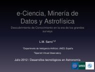
Figure 2.1: Large scale image <strong>of</strong> M101. The grayscale is the Digital Sky Survey image and the<br />
contour image is the H i from the VLA (Braun, 1995). NGC 5471 is loc<strong>at</strong>ed <strong>in</strong> the outskirts <strong>of</strong> the<br />
galaxy, <strong>in</strong> an arm concentr<strong>at</strong>ion <strong>of</strong> H i.<br />
the <strong>study</strong> <strong>of</strong> the <strong>in</strong>terrel<strong>at</strong>ion between stars, gas and dust components is highly relevant to<br />
understand the n<strong>at</strong>ure <strong>of</strong> these <strong>regions</strong>.<br />
30 Doradus <strong>in</strong> the Large Magellanic Cloud (LMC) and NGC 604 <strong>in</strong> M33 are the two<br />
largest GEHRs <strong>in</strong> the Local Group and they have been the subject <strong>of</strong> very detailed analyses.<br />
Both are dom<strong>in</strong><strong>at</strong>ed by very young (2-4 Myr) ioniz<strong>in</strong>g stellar popul<strong>at</strong>ions, but they<br />
present two r<strong>at</strong>her <strong>different</strong> stellar distributions. While NGC 604 is an extended Scaled OB<br />
Associ<strong>at</strong>ion (SOBA) with ∼ 200 O+WR massive stars surrounded by nebular filamentary<br />
structures, 30 Doradus is powered by a Super Star Cluster (SSC) – a much more compact<br />
core (Maíz-Apellániz, 2001) – and a halo, with <strong>different</strong> stellar popul<strong>at</strong>ions rang<strong>in</strong>g from<br />
2 to 20 Myr (Walborn and Blades, 1997). Both GEHRs <strong>in</strong>clude an ongo<strong>in</strong>g star form<strong>at</strong>ion<br />
with young stars still embedded <strong>in</strong> their parent molecular cloud. The structural similarities<br />
and differences between these well studied and <strong>sp<strong>at</strong>ially</strong> well <strong>resolved</strong> Local Group GEHRs<br />
have made them obvious ideal labor<strong>at</strong>ories <strong>in</strong> which to <strong>study</strong> massive star form<strong>at</strong>ion, but <strong>in</strong>
2.2. Observ<strong>at</strong>ions and D<strong>at</strong>a Reduction 13<br />
order to extrapol<strong>at</strong>e our knowledge to distant lum<strong>in</strong>ous un<strong>resolved</strong> starbursts it is critically<br />
necessary to go a step further and to analyze <strong>in</strong> detail the somewh<strong>at</strong> more distant GEHRs<br />
just outside the neighbourhood <strong>of</strong> the Local Group.<br />
M101 (NGC 5457) is a giant spiral galaxy loc<strong>at</strong>ed <strong>at</strong> a distance <strong>of</strong> 7.2 Mpc (Stetson<br />
et al., 1998), yield<strong>in</strong>g a l<strong>in</strong>ear scale <strong>of</strong> 34.9 pc/ ′′ .This galaxy conta<strong>in</strong>s a large number <strong>of</strong> very<br />
lum<strong>in</strong>ous GEHRs, <strong>of</strong> which NGC 5471 (α 2000 = 14 h 04 m 29 s , δ 2000 = +54 ◦ 23 ′ 48 ′′ ; l = 101. ◦ 78, b<br />
= +59. ◦ 63) is one <strong>of</strong> the outermost, <strong>at</strong> a galactocentric radius <strong>of</strong> about 25 kpc (see Figure 2.1).<br />
The Hα morphology <strong>of</strong> NGC 5471 shows multiple cores with surround<strong>in</strong>g nebular filaments,<br />
extend<strong>in</strong>g over a diameter <strong>of</strong> ∼ 17 ′′ , or ∼ 600 pc. Ground-based photometry shows five bright<br />
knots, design<strong>at</strong>ed by Skillman (1985) as components A, B, C, D and E. Component A is as<br />
lum<strong>in</strong>ous as 30 Doradus, while components B, C and E are comparable to NGC 604, the two<br />
prototypical <strong>sp<strong>at</strong>ially</strong> <strong>resolved</strong> m<strong>in</strong>i-starbursts <strong>in</strong> the Local Group. Thus NGC 5471 is truly<br />
a giant star form<strong>in</strong>g region.<br />
All these fe<strong>at</strong>ures make <strong>of</strong> NGC 5471 an excellent candid<strong>at</strong>e for the <strong>study</strong> <strong>of</strong> complex<br />
star form<strong>at</strong>ion, be<strong>in</strong>g close to the limit distance between the <strong>sp<strong>at</strong>ially</strong> well <strong>resolved</strong> Local<br />
Group GEHRs and the more distant un<strong>resolved</strong> starbursts, thus provid<strong>in</strong>g an <strong>in</strong>termedi<strong>at</strong>e<br />
step <strong>in</strong> our understand<strong>in</strong>g <strong>of</strong> very massive star form<strong>in</strong>g <strong>regions</strong>.<br />
This chapter is organized as follows. Section 2.2 describes the observ<strong>at</strong>ions and d<strong>at</strong>a<br />
reduction. Section 2.3 presents the <strong>in</strong>tegr<strong>at</strong>ed analysis <strong>of</strong> both the <strong>in</strong>dividual large clusters<br />
and the whole <strong>of</strong> NGC 5471, and the photometry <strong>of</strong> the <strong>resolved</strong> stars. The results found <strong>in</strong><br />
section 2.3 are elabor<strong>at</strong>ed and discussed <strong>in</strong> section 2.4.<br />
2.2 Observ<strong>at</strong>ions and D<strong>at</strong>a Reduction<br />
For NGC 5471 we have obta<strong>in</strong>ed near <strong>in</strong>frared JHK images and have retrieved the broad<br />
and narrow band optical images available <strong>in</strong> the HST archive. Ultraviolet NUV and FUV<br />
images <strong>of</strong> M101 have also been retrieved from the GALEX archive.<br />
2.2.1 GALEX d<strong>at</strong>a<br />
The Galaxy Evolution Explorer (GALEX) far-ultraviolet (FUV; λ ref = 1530 Å, ∆λ =<br />
400 Å) and near-ultraviolet (NUV; λ ref = 2310 Å, ∆λ = 1000 Å) images <strong>of</strong> M101 were<br />
retrieved from the Nearby Galaxies Survey (NGS).<br />
The GALEX <strong>in</strong>strument is described by Mart<strong>in</strong> et al. (2005) and its on-orbit performance<br />
by Morrissey et al. (2005). GALEX FUV and NUV imag<strong>in</strong>g was obta<strong>in</strong>ed with total exposure<br />
times <strong>of</strong> 1041 s <strong>in</strong> each band. The 1σ NUV (FUV) sensitivity limit <strong>of</strong> the GALEX images is<br />
27.6 (27.5) AB mag arcsec −2 for these d<strong>at</strong>a (Bianchi et al., 2005). At the distance <strong>of</strong> M101,<br />
the l<strong>in</strong>ear scale <strong>of</strong> 34.9 pc/ ′′ implies th<strong>at</strong> the GALEX po<strong>in</strong>t spread function (PSF) <strong>of</strong> 4.6<br />
arcsec transl<strong>at</strong>es to 160 pc; this is barely sufficient to resolve some <strong>of</strong> the structure <strong>in</strong> NGC
14 2 • The star form<strong>at</strong>ion history <strong>of</strong> NGC 5471<br />
Filter Band Exposure (s) Observ<strong>at</strong>ion ID<br />
F547M Strömgren y 2 × 600 U4DN030DR, U4DN030ER<br />
2 × 100 U4DN030FR, U4DN030GR<br />
20 U4DN030HM<br />
F675W WFPC2 R 2 × 400 U4DN0308R, U4DN0309R<br />
2 × 50 U4DN030AR, U4DN030BR<br />
10 U4DN030CR<br />
F656N Hα 180 U4DN0305R<br />
2 × 600 U4DN0306R, U4DN0307R<br />
F673N [S II] 3 × 700 U4DN0301R, U4DN0302R, U4DN0303R<br />
300 U4DN0304R<br />
Table 2.1: Journal <strong>of</strong> HST/WFPC2 observ<strong>at</strong>ions <strong>of</strong> NGC 5471. All images were obta<strong>in</strong>ed on 1997<br />
November 1 for the cycle 6 program GO-6928, with You-Hua Chu as PI. The object <strong>of</strong> <strong>study</strong> is<br />
centered <strong>in</strong> the WF3 camera.<br />
5471, and we will only use the GALEX d<strong>at</strong>a to <strong>study</strong> the <strong>in</strong>tegr<strong>at</strong>ed photometry.<br />
2.2.2 HST/WFPC2 Imag<strong>in</strong>g<br />
Hubble Space Telescope (HST) Wide Field Planetary Camera 2 (WFPC2) images <strong>of</strong><br />
NGC 5471 were retrieved from the HST archive. The images were taken on 1997 November<br />
1 through two emission-l<strong>in</strong>e filters: F656N (Hα) and F673N ([S II]), and two cont<strong>in</strong>uum<br />
filters: F547M (Strömgren y) and F675W (WFPC2 R) (Heyer, 2004). Each camera images<br />
onto a Loral 800×800 CCD which gives a pl<strong>at</strong>e scale <strong>of</strong> 0. ′′ 046 pixel −1 for the PC camera and<br />
0. ′′ 10 pixel −1 for the three WF cameras, with a readout noise <strong>of</strong> ∼5 e − and a ga<strong>in</strong> <strong>of</strong> 7 e − /DN<br />
for this observ<strong>at</strong>ions. NGC 5471 is centered <strong>in</strong> the WF3 camera <strong>in</strong> all images. The scale <strong>of</strong><br />
the WF CCDs <strong>at</strong> NGC 5471, for which we assume a distance modulus <strong>of</strong> (m − M) = 29.3<br />
(Stetson et al., 1998), is 3.5 pc pixel −1 . Table 2.1 lists the details concern<strong>in</strong>g the WFPC2<br />
d<strong>at</strong>a.<br />
The HST pipel<strong>in</strong>e processed WFPC2 images were subjected to the usual process<strong>in</strong>g us<strong>in</strong>g<br />
the IRAF 1 and STSDAS 2 s<strong>of</strong>tware packages, follow<strong>in</strong>g the procedures outl<strong>in</strong>ed <strong>in</strong> the HST<br />
D<strong>at</strong>a Handbook. We used the multiple exposures to correct for the <strong>in</strong>cidence <strong>of</strong> cosmic rays<br />
as well as to elim<strong>in</strong><strong>at</strong>e hotpixels and other defects on the CCD. We f<strong>in</strong>ally co-added the<br />
images to produce deep mosaics.<br />
Given the lum<strong>in</strong>osity <strong>of</strong> NGC 5471, its Hα and [SII] emission contributes significantly<br />
1 IRAF is distributed by the N<strong>at</strong>ional Optical Observ<strong>at</strong>ory, which is oper<strong>at</strong>ed by the Associ<strong>at</strong>ion <strong>of</strong> Universities<br />
for Research <strong>in</strong> Astronomy, Inc., under cooper<strong>at</strong>ive agreement with the N<strong>at</strong>ional Science Found<strong>at</strong>ion.<br />
2 Space Telescope Science D<strong>at</strong>a Analysis System (STSDAS) is a product <strong>of</strong> the Space Telescope Science<br />
Institute, oper<strong>at</strong>ed by AURA for NASA.
2.2. Observ<strong>at</strong>ions and D<strong>at</strong>a Reduction 15<br />
Figure 2.2: HST WFPC2 images <strong>of</strong> NGC 5471 <strong>in</strong> cont<strong>in</strong>uum corrected nebular filters Hα (F656N),<br />
[SII] (F673N), and emission l<strong>in</strong>e corrected cont<strong>in</strong>uum filters F547M and F675W ′ . The five knots from<br />
Skillman (1985) are marked <strong>in</strong> the Hα image. An ellipse <strong>in</strong>dic<strong>at</strong><strong>in</strong>g the core <strong>of</strong> the region is drawn <strong>in</strong><br />
the Hα and F675W ′ images. North is up and east to the left.<br />
to the broad band (F675W) image. To elim<strong>in</strong><strong>at</strong>e the nebular contribution from the broad<br />
band and to produce cont<strong>in</strong>uum-free Hα and [SII] emission l<strong>in</strong>e images, we followed the<br />
procedure described below. First we multiplied the images by the PHOTFLAM parameter<br />
obta<strong>in</strong>ed by synphot to convert from count r<strong>at</strong>es to flux densities, and then divided them by<br />
its time exposure. From the SYNPHOT task <strong>in</strong> STSDAS we determ<strong>in</strong>ed the filter widths,<br />
and multiplied the flux densities found by the correspond<strong>in</strong>g filter widths <strong>in</strong> order to obta<strong>in</strong><br />
fluxes. The correct filter widths are the filter rectangular width RECTW (Luridiana et al.,<br />
2003). RECTW is def<strong>in</strong>ed as the width <strong>in</strong> Ångstroms <strong>of</strong> a rectangle with the same total area<br />
as the total transmission curve and a height given by the peak <strong>in</strong> the curve. We then scaled<br />
the Hα, [S II] and F675W images and performed an iter<strong>at</strong>ive subtraction to obta<strong>in</strong> a new,
16 2 • The star form<strong>at</strong>ion history <strong>of</strong> NGC 5471<br />
Figure 2.3: Color composite <strong>of</strong> HST WFPC2 images <strong>of</strong> NGC 5471. Each image has its own filter comb<strong>in</strong><strong>at</strong>ion label, <strong>in</strong> the usual RGB (Red, Green,<br />
Blue) color sequence . North is up, and east to the left.
2.2. Observ<strong>at</strong>ions and D<strong>at</strong>a Reduction 17<br />
Band Time (UT) Dur<strong>at</strong>ion (s) Air mass<br />
J 04:09:00 1 × 60 1.38<br />
H 01:03:08 3 × 15 1.11<br />
K s 21:59:29 10 × 5 1.31<br />
Table 2.2: Journal <strong>of</strong> TNG/ARNICA observ<strong>at</strong>ions <strong>of</strong> NGC 5471.<br />
emission l<strong>in</strong>e free, broad band image (F675W ′ ).<br />
Figure 2.2 shows NGC 5471 <strong>in</strong> the four bands. An ellipse <strong>in</strong>dic<strong>at</strong><strong>in</strong>g the core <strong>of</strong> the<br />
region is drawn <strong>in</strong> the Hα and F675W ′ images. The five brightest components first noted<br />
by Skillman (1985) and design<strong>at</strong>ed as A, B, C, D and E, are dist<strong>in</strong>ctly observed <strong>in</strong> the Hα<br />
image. The presence <strong>of</strong> a supernova remnant (NGC 5471B) is clearly seen as an <strong>in</strong>tense [SII]<br />
emission source <strong>in</strong> the B-component <strong>in</strong> the F673N image. Previous works have associ<strong>at</strong>ed X-<br />
ray sources with supernova remnants (SNRs) <strong>in</strong> M101. Chen et al. (2002) conclude th<strong>at</strong> the<br />
energetic SNR <strong>in</strong> NGC 5471B (first identified by Skillman, 1985) was very likely produced by<br />
a hypernova, an explosion one or two orders <strong>of</strong> magnitude brighter than the canonical 10 51<br />
erg energy explosion associ<strong>at</strong>ed with a normal SN, although this result has been questioned<br />
recently (Jenk<strong>in</strong>s et al., 2004).<br />
Several color images <strong>of</strong> NGC 5471 are shown <strong>in</strong> Figure 3.1. Each image has its own filter<br />
comb<strong>in</strong><strong>at</strong>ion label, which <strong>in</strong>dic<strong>at</strong>es the used filters <strong>in</strong> the composition <strong>in</strong> the usual RGB (Red,<br />
Green, Blue) color sequence.<br />
2.2.3 Near-<strong>in</strong>frared photometry<br />
JHK s photometry was performed on 2000 April 29, us<strong>in</strong>g the 3.58m TNG (Telescopio<br />
Nazionale Galileo) <strong>at</strong> the Observ<strong>at</strong>orio del Roque de los Muchachos <strong>in</strong> La Palma. The camera<br />
used was ARNICA (ARcetri Near Infrared CAmera), with a CCD detector NICMOS<br />
256×256 HgCdTe and ga<strong>in</strong> <strong>of</strong> 19 e − /ADU. The sp<strong>at</strong>ial scale was 0. ′′ 35 pixel −1 and the field<br />
<strong>of</strong> view 90×90 arcsec 2 . The details <strong>of</strong> these observ<strong>at</strong>ions are given <strong>in</strong> Table 2.2.<br />
The flux calibr<strong>at</strong>ion <strong>of</strong> the images has been done us<strong>in</strong>g 2MASS images <strong>of</strong> NGC 5471,<br />
retrieved from the 2MASS Extended Source C<strong>at</strong>alog. We first measured the <strong>in</strong>tegr<strong>at</strong>ed flux<br />
<strong>of</strong> the 2MASS images <strong>in</strong> a circle conta<strong>in</strong><strong>in</strong>g the region and then, we used th<strong>at</strong> aperture<br />
centered <strong>in</strong> the same coord<strong>in</strong><strong>at</strong>es and cover<strong>in</strong>g the same area <strong>in</strong> the ARNICA images. We<br />
obta<strong>in</strong>ed the photometric constants compar<strong>in</strong>g the calibr<strong>at</strong>ed 2MASS fluxes with those from<br />
ARNICA by means <strong>of</strong> the transform<strong>at</strong>ion equ<strong>at</strong>ions <strong>of</strong> the two systems.<br />
In order to compare the two sets <strong>of</strong> optical and NIR d<strong>at</strong>a, we aligned the HST and TNG<br />
images. We degraded the WFPC2 images to the sp<strong>at</strong>ial scale and see<strong>in</strong>g <strong>of</strong> the IR ones,<br />
then we identified several objects <strong>in</strong> both d<strong>at</strong>a sets and marked them with the IRAF center<br />
rout<strong>in</strong>e. Next, we aligned the images with the geomap and geotran rout<strong>in</strong>es, us<strong>in</strong>g the HST
18 2 • The star form<strong>at</strong>ion history <strong>of</strong> NGC 5471<br />
J H<br />
10" ~ 350 pc<br />
17" ~ 600 pc<br />
Figure 2.4: JHKs grayscale images and contour plots. The isophotes range from 20 up to 100 per cent <strong>of</strong> the peak value <strong>of</strong> the image.
2.3. Results 19<br />
images as reference.<br />
Figure 2.4 shows the images and contour plots <strong>of</strong> the <strong>in</strong>frared bands. The multiple knots<br />
present <strong>in</strong> these images are well identified with those <strong>in</strong> Figure 2.2 <strong>in</strong> the F547M and F673W ′<br />
filters.<br />
2.3 Results<br />
2.3.1 Cluster Photometry<br />
We have derived the <strong>in</strong>tegr<strong>at</strong>ed magnitudes and colors <strong>in</strong> eleven <strong>different</strong> apertures cover<strong>in</strong>g<br />
the ma<strong>in</strong> components <strong>in</strong> the core <strong>of</strong> NGC 5471. The apertures were chosen and def<strong>in</strong>ed<br />
<strong>in</strong> the H-band image, maximiz<strong>in</strong>g the area <strong>in</strong> order to <strong>in</strong>clude the fe<strong>at</strong>ures <strong>of</strong> all images,<br />
s<strong>in</strong>ce there were some small <strong>of</strong>fsets <strong>in</strong> the position and <strong>in</strong>tensity <strong>of</strong> the knots <strong>in</strong> the optical<br />
and <strong>in</strong>frared images respectively. Then, the same polygons were used for the J, K s and HST<br />
images. Polygons were marked by us<strong>in</strong>g the IRAF task polymark and the <strong>in</strong>tegr<strong>at</strong>ed magnitudes<br />
were computed us<strong>in</strong>g the IRAF task polyphot. The <strong>in</strong>tegr<strong>at</strong>ed magnitudes <strong>of</strong> the<br />
HST images are given <strong>in</strong> the VEGAMAG system. The polygons def<strong>in</strong>ed are shown <strong>in</strong> Figure<br />
2.5.<br />
The <strong>in</strong>tegr<strong>at</strong>ed magnitudes and colors derived <strong>in</strong> each area were corrected for the Galactic<br />
foreground ext<strong>in</strong>ction toward M101 us<strong>in</strong>g the color excess E(B-V) = 0.01 (Schlegel et al.,<br />
1998), although its effect is negligible. The absorption coefficients for the 5 bands were derived<br />
assum<strong>in</strong>g R V = A V /E(B −V ) = 3.1, and us<strong>in</strong>g the A λ curve from Cardelli et al. (1989). The<br />
uncerta<strong>in</strong>ty <strong>of</strong> the <strong>in</strong>dividual fluxes have been computed <strong>in</strong>clud<strong>in</strong>g the Poisson photon count<br />
error, the uncerta<strong>in</strong>ty on the background sett<strong>in</strong>g and the photometric calibr<strong>at</strong>ion uncerta<strong>in</strong>ty.<br />
Results <strong>of</strong> the <strong>in</strong>tegr<strong>at</strong>ed photometry <strong>in</strong> the five bands are given <strong>in</strong> Table 2.3.<br />
We also have measured the Hα flux for each polygon. To measure the <strong>in</strong>tegr<strong>at</strong>ed Hα flux<br />
<strong>of</strong> the whole region, we have decontam<strong>in</strong><strong>at</strong>ed the F656N image from the broad band F675W<br />
contribution. Then, we have then plotted the contour <strong>at</strong> 3σ from the sky (with isophotal flux<br />
6.3 × 10 −15 erg cm −2 s −1 arcsec −1 ) and found the circular aperture centered <strong>in</strong> the region<br />
th<strong>at</strong> best fits th<strong>at</strong> isophotal contour. The radius <strong>of</strong> this aperture is 15 arcsec from the center<br />
(see Figure 2.6). The flux measured <strong>in</strong>side this circular aperture is (3.65 ± 0.17) × 10 −12 erg<br />
cm −2 s −1 . We have used the PHOTFLAM value given by synphot and a value <strong>of</strong> RECTW <strong>of</strong><br />
28.3 Å. Measured Hα fluxes for each <strong>of</strong> the polygonal selections and the parameter derived<br />
from them are given <strong>in</strong> Table 2.4. The effective radii (R eff ) <strong>of</strong> a polygon is def<strong>in</strong>ed as the<br />
radii <strong>of</strong> a circular aperture <strong>of</strong> the same area.<br />
S<strong>in</strong>ce GALEX images do not have enough resolution, we were not able to get the fluxes<br />
for each polygon. As <strong>in</strong> the case <strong>of</strong> the nebular flux, we measured the FUV and NUV fluxes<br />
<strong>in</strong>side 15 ′′ radii apertures centered <strong>in</strong> NGC 5471. We obta<strong>in</strong> a FUV flux <strong>of</strong> (9.9±0.1)×10 −14<br />
erg cm −2 s −1 Å −1 (14.19 ± 0.05 AB magnitudes) and a NUV flux <strong>of</strong> (4.5 ± 0.1) × 10 −14 erg
20 2 • The star form<strong>at</strong>ion history <strong>of</strong> NGC 5471<br />
Figure 2.5: Plot <strong>of</strong> the eleven polygons, limit<strong>in</strong>g the <strong>different</strong> areas where the <strong>in</strong>tegr<strong>at</strong>ed magnitudes<br />
are computed. The numbers belong to our own def<strong>in</strong>ition while the A, B, C, D and E letters are the<br />
knots identified by Skillman (1985). The hypernova is loc<strong>at</strong>ed <strong>in</strong> knot 6.<br />
cm −2 s −1 Å −1 (14.24 ± 0.05 AB magnitudes).<br />
In order to use these values <strong>in</strong> the analysis, we need to transform AB magnitudes to the<br />
VEGAMAG system. The transform<strong>at</strong>ion formula is (Maíz-Apellániz, 2007):<br />
AB p = (m p − ZP p ) + AB p (V ega) (2.1)<br />
where AB p is the magnitude <strong>of</strong> the object <strong>in</strong> the AB system and filter passband p, m p the<br />
magnitude <strong>of</strong> the object <strong>in</strong> filter p us<strong>in</strong>g Vega as reference spectral energy distribution (SED),<br />
ZP p is the zero po<strong>in</strong>t <strong>of</strong> the p filter <strong>in</strong> the Vega system and AB p (Vega) is the AB magnitude<br />
<strong>of</strong> Vega <strong>in</strong> filter p. This magnitude is given by:
2.3. Results 21<br />
Aperture J H K s m 547M m 675W m 675W ′<br />
N5471-1 16.43 ± 0.11 16.26 ± 0.12 16.03 ± 0.14 16.66 ± 0.06 15.56 ± 0.06 16.30 ± 0.06<br />
N5471-2 16.90 ± 0.11 16.57 ± 0.12 16.48 ± 0.14 17.21 ± 0.06 16.30 ± 0.06 16.94 ± 0.06<br />
N5471-3 17.35 ± 0.11 17.09 ± 0.12 17.12 ± 0.14 17.22 ± 0.06 16.84 ± 0.06 17.11 ± 0.06<br />
N5471-4 17.52 ± 0.11 17.08 ± 0.12 16.99 ± 0.14 18.17 ± 0.06 17.07 ± 0.06 17.77 ± 0.06<br />
N5471-5 17.83 ± 0.11 17.28 ± 0.12 17.27 ± 0.14 18.58 ± 0.06 17.59 ± 0.06 18.16 ± 0.06<br />
N5471-6 17.34 ± 0.11 17.21 ± 0.12 17.00 ± 0.14 17.62 ± 0.06 16.41 ± 0.06 17.12 ± 0.06<br />
N5471-7 16.98 ± 0.11 16.59 ± 0.12 16.47 ± 0.14 17.56 ± 0.06 16.49 ± 0.06 17.10 ± 0.06<br />
N5471-8 17.89 ± 0.11 17.41 ± 0.12 17.39 ± 0.14 18.70 ± 0.06 17.68 ± 0.06 18.22 ± 0.06<br />
N5471-9 19.15 ± 0.13 18.63 ± 0.13 18.63 ± 0.15 20.23 ± 0.06 18.71 ± 0.06 19.54 ± 0.06<br />
N5471-10 18.14 ± 0.11 17.80 ± 0.12 17.57 ± 0.15 18.63 ± 0.06 17.45 ± 0.06 18.22 ± 0.06<br />
N5471-11 18.55 ± 0.12 18.00 ± 0.12 18.11 ± 0.15 19.27 ± 0.06 18.40 ± 0.06 18.84 ± 0.06<br />
NGC 5471 14.14 ± 0.10 13.84 ± 0.12 13.74 ± 0.14 14.67 ± 0.06 13.62 ± 0.06 14.27 ± 0.06<br />
Table 2.3: Integr<strong>at</strong>ed magnitudes and Hα flux for the eleven <strong>regions</strong> <strong>of</strong> NGC 5471. Magnitudes<br />
from HST are given <strong>in</strong> the VEGAMAG system. Results for m 675W ′ column were measured from<br />
the emission l<strong>in</strong>e free F675W image. The last row belongs to the <strong>in</strong>tegr<strong>at</strong>ed magnitude <strong>of</strong> the whole<br />
region.<br />
(∫ )<br />
Pp (λ)f λ,V ega (λ)λdλ<br />
AB p (V ega) = −2.5 log 10 ∫<br />
Pp (λ)(cf ν,AB /λ)dλ<br />
(2.2)<br />
where P p (λ) is the dimensionless filter sensitivity function <strong>of</strong> filter p, f λ,V ega (λ) is the Vega<br />
spectrum and f ν,AB = 3.63079 × 10 −20 erg s −1 cm −2 Hz −1 is the reference spectral energy<br />
distribution <strong>of</strong> the AB system.<br />
We have used FUV and NUV filter passbands to calcul<strong>at</strong>e the AB magnitudes <strong>of</strong> Vega<br />
by means <strong>of</strong> equ<strong>at</strong>ion 2.2. As the zero po<strong>in</strong>ts for GALEX are ZP = 0.000 <strong>in</strong> both bands, we<br />
have<br />
m F UV = AB F UV − 2.073 (2.3)<br />
m NUV = AB NUV − 1.647 (2.4)<br />
F<strong>in</strong>ally, the GALEX VEGAMAG magnitudes <strong>of</strong> NGC 5471 used below are m F UV =<br />
12.12 and m NUV = 12.59.<br />
The <strong>in</strong>tegr<strong>at</strong>ed photometric measurements have been analyzed with the help <strong>of</strong> CHORI-<br />
ZOS 3 , a code written <strong>in</strong> IDL by Maíz-Apellániz (2004). This code compares photometric<br />
d<strong>at</strong>a with model spectral energy distributions (SEDs), calcul<strong>at</strong><strong>in</strong>g the likelihood for the full<br />
parameter range specified, allow<strong>in</strong>g for the identific<strong>at</strong>ion <strong>of</strong> multiple solutions. In general,<br />
models are parameterized <strong>in</strong> terms <strong>of</strong> physical quantities: some <strong>of</strong> them are <strong>in</strong>tr<strong>in</strong>sic, i.e. they<br />
might depend on the n<strong>at</strong>ure and distance to the objects (e.g. age, metallicity, . . . ), while<br />
3 CHi-square cOde for parameteRized model<strong>in</strong>g and characterIZ<strong>at</strong>ion <strong>of</strong> phOtometry and Spectrophotmetry.<br />
The l<strong>at</strong>est version can be obta<strong>in</strong>ed from http://www.iaa.es/∼jmaiz
22 2 • The star form<strong>at</strong>ion history <strong>of</strong> NGC 5471<br />
Figure 2.6: Cont<strong>in</strong>uum free Hα image <strong>of</strong> NGC 5471. The circular aperture <strong>of</strong> 15 ′′ where the <strong>in</strong>tegr<strong>at</strong>ed<br />
photometry was performed to obta<strong>in</strong> the total flux is overplotted. The ellipse <strong>in</strong>dic<strong>at</strong><strong>in</strong>g the<br />
core <strong>of</strong> the region is drawn as reference.<br />
others are extr<strong>in</strong>sic and depend on the properties <strong>of</strong> the <strong>in</strong>terstellar m<strong>at</strong>ter (redden<strong>in</strong>g and<br />
ext<strong>in</strong>ction law). CHORIZOS can handle SED families for stellar <strong>at</strong>mospheres and clusters<br />
(Starburst99; Leitherer et al., 1999) and uses χ 2 m<strong>in</strong>imiz<strong>at</strong>ion to f<strong>in</strong>d all models comp<strong>at</strong>ible<br />
with the observed d<strong>at</strong>a <strong>in</strong> a (2 <strong>in</strong>tr<strong>in</strong>sic +2 extr<strong>in</strong>sic)-dimensional parameter space. It<br />
<strong>in</strong>cludes a wide list <strong>of</strong> filters for <strong>different</strong> systems (Johnson-Cous<strong>in</strong>s, HST/WFPC2, 2MASS,<br />
. . . ) and allows for published magnitudes to be used directly. For a set <strong>of</strong> objects with<br />
measured magnitudes m 1 , m 2 , . . . , m M+1 (with <strong>in</strong>dependent uncerta<strong>in</strong>ties σ 1 , σ 2 , . . . , σ M+1 ),<br />
derived <strong>in</strong>dependent colors c 1 , c 2 , . . . , c M , and a set <strong>of</strong> N parameters with M > N, no strict<br />
solutions, but only approxim<strong>at</strong>e ones, can be found s<strong>in</strong>ce the problem has more equ<strong>at</strong>ions<br />
or sets <strong>of</strong> model parameters th<strong>at</strong> produce a given color than model parameters. Hence, the<br />
code f<strong>in</strong>ds the N-volume <strong>of</strong> approxim<strong>at</strong>e solutions by us<strong>in</strong>g χ 2 m<strong>in</strong>imiz<strong>at</strong>ion.<br />
The first step <strong>of</strong> the program is to read the unreddened SED models, ext<strong>in</strong>guish them<br />
accord<strong>in</strong>g to a given ext<strong>in</strong>ction law, and obta<strong>in</strong> the synthetic photometry; the code <strong>in</strong>cludes<br />
pre-calcul<strong>at</strong>ed tables for all the models and filters. To run the program, CHORIZOS requires
2.3. Results 23<br />
Aperture R eff F(Hα) L(Hα) Q(H 0 ) M ii EW(Hα)<br />
pc 10 −13 erg s −1 cm −2 10 39 erg s −1 10 51 s −1 10 4 M ⊙ Å<br />
NGC5471-1 61.1 6.63 ± 0.31 4.1 4.1 13.0 1187 ± 77<br />
NGC5471-2 60.9 3.07 ± 0.14 1.9 1.9 6.1 993 ± 64<br />
NGC5471-3 47.0 0.93 ± 0.04 0.6 0.6 1.9 354 ± 23<br />
NGC5471-4 51.2 1.59 ± 0.07 1.0 1.0 3.2 1103 ± 71<br />
NGC5471-5 46.0 0.79 ± 0.04 0.5 0.5 1.6 788 ± 51<br />
NGC5471-6 58.9 2.42 ± 0.11 1.5 1.5 4.8 919 ± 59<br />
NGC5471-7 63.1 2.34 ± 0.11 1.5 1.4 4.7 872 ± 57<br />
NGC5471-8 43.5 0.72 ± 0.03 0.5 0.4 1.4 756 ± 49<br />
NGC5471-9 34.0 0.38 ± 0.02 0.2 0.2 0.8 1369 ± 90<br />
NGC5471-10 46.2 1.22 ± 0.06 0.8 0.8 2.4 1282 ± 83<br />
NGC5471-11 53.6 0.31 ± 0.01 0.2 0.2 0.6 585 ± 37<br />
NGC 5471 525 36.5 ± 1.70 23 22 73 783 ± 40<br />
Table 2.4: Integr<strong>at</strong>ed Hα flux and derived parameters for the eleven <strong>regions</strong> <strong>of</strong> NGC 5471. R eff is<br />
the effective radius <strong>of</strong> the polygon. The last row belongs to the <strong>in</strong>tegr<strong>at</strong>ed values <strong>of</strong> the whole region.<br />
a file with the photometry d<strong>at</strong>a and a series <strong>of</strong> <strong>in</strong>put parameters, such as the model family,<br />
understood as the collection <strong>of</strong> SED from stellar <strong>at</strong>mosphere models or synthetic stellar<br />
popul<strong>at</strong>ions, and the range <strong>of</strong> the parameters to be used. Then, CHORIZOS reads the model<br />
photometry from the tables calcul<strong>at</strong>ed previously, <strong>in</strong>terpol<strong>at</strong>es, calcul<strong>at</strong>es the likelihood for<br />
each grid po<strong>in</strong>t, and write the results for each <strong>of</strong> the four parameters (mode, mean, standard<br />
devi<strong>at</strong>ion, median, . . . ). The program conta<strong>in</strong>s a useful module which reads the results and<br />
produces spectra, probability contour plots and additional st<strong>at</strong>istics.<br />
In the case <strong>of</strong> our <strong>study</strong>, we have used the STARBURST99 models (Leitherer et al., 1999)<br />
with the implement<strong>at</strong>ion by Smith et al. (2002) which <strong>in</strong>cludes a grid <strong>of</strong> blanketed stellar<br />
<strong>at</strong>mospheres <strong>at</strong> <strong>different</strong> metallicities. We fixed two parameters: the known metallicity <strong>of</strong><br />
NGC 5471 and the type <strong>of</strong> dust, leav<strong>in</strong>g unconstra<strong>in</strong>ed the amount <strong>of</strong> ext<strong>in</strong>ction and the<br />
age.<br />
Regard<strong>in</strong>g ext<strong>in</strong>ction, CHORIZOS works with E(4405 − 5495) and R 5495 , which are the<br />
monochrom<strong>at</strong>ic equivalent to E(B − V ) and R V respectively, the values 4405 and 5495<br />
referr<strong>in</strong>g to the central wavelength (<strong>in</strong> Å) <strong>of</strong> the B and V filters. We used the standard type<br />
<strong>of</strong> dust characterized by a value R 5495 = 3.1. The metallicity <strong>of</strong> the region was assumed to<br />
be traced by the oxygen abundance. Recent deriv<strong>at</strong>ions from detailed spectrophotometric<br />
studies give a mean value <strong>of</strong> 12+log(O/H) <strong>of</strong> 8.06 ± 0.03 for components A, C and D;<br />
a slightly lower abundance <strong>of</strong> 7.94 ± 0.03 is found for component B (Kennicutt et al.,<br />
2003). These values correspond to about 0.25 the solar oxygen abundance, if the value by<br />
Asplund et al. (2005) for the solar oxygen abundance is assumed. Therefore we used the
24 2 • The star form<strong>at</strong>ion history <strong>of</strong> NGC 5471<br />
value Z = 0.2Z ⊙ <strong>in</strong> CHORIZOS.<br />
2.3.2 Resolved Stellar Photometry<br />
WFPC2 Photometry<br />
The stellar photometric analysis was performed with the HSTphot package (Dolph<strong>in</strong>,<br />
2000b). This package is specifically designed for use with HST WFPC2 images. It uses a<br />
library <strong>of</strong> T<strong>in</strong>y Tim (Krist, 1995) undersampled po<strong>in</strong>t-spread functions (PSFs) for <strong>different</strong><br />
loc<strong>at</strong>ions <strong>of</strong> the star on the camera and <strong>of</strong> the star center with<strong>in</strong> the pixel, to center the<br />
star and to f<strong>in</strong>d its magnitude, given <strong>in</strong> the flight system magnitude. It also conta<strong>in</strong>s several<br />
programs for general reduction procedures. The first step is to run the mask task to mask<br />
out the bad pixels and other image defects identified <strong>in</strong> the d<strong>at</strong>a quality images. The sky<br />
comput<strong>at</strong>ion is made by getsky, which takes all pixels <strong>in</strong> an annulus around each pixel,<br />
determ<strong>in</strong>es the sky value and calcul<strong>at</strong>es the sky background map. The next step is to run<br />
crmask for cosmic ray removal, which uses the sky file cre<strong>at</strong>ed by getsky. It has the capability<br />
<strong>of</strong> clean<strong>in</strong>g images th<strong>at</strong> are not perfectly aligned, and it can handle images from <strong>different</strong><br />
filters. To comb<strong>in</strong>e multiple images per filter and to produce a f<strong>in</strong>al deep image per filter,<br />
the coadd procedure was used. The f<strong>in</strong>al step requires the hotpixels procedure, which uses<br />
the result from getsky and tries to loc<strong>at</strong>e and remove all hot pixels. This is an important<br />
step, s<strong>in</strong>ce hot pixels can cre<strong>at</strong>e false detections and also, can throw <strong>of</strong>f the PSF solutions.<br />
The hstphot rout<strong>in</strong>e was run on the images <strong>in</strong> the F547M and F675W ′ bands. This<br />
task performs stellar PSF photometry on multiple images from <strong>different</strong> filters, <strong>in</strong>clud<strong>in</strong>g<br />
alignment and aperture corrections, as well as PSF modific<strong>at</strong>ions to correct for errors <strong>of</strong><br />
geometric distortion via the Holtzman et al. (1995) distortion correction equ<strong>at</strong>ions and the<br />
34th row error, noted by Shaklan et al. (1995) (see also Anderson and K<strong>in</strong>g, 1999), and<br />
correction for charge transfer <strong>in</strong>efficiency (Dolph<strong>in</strong>, 2000a). There are several parameters to<br />
use dur<strong>in</strong>g the run <strong>of</strong> hstphot. We enabled the determ<strong>in</strong><strong>at</strong>ion <strong>of</strong> the “local sky” (from now<br />
on, nebular case), because <strong>of</strong> the rapidly-vary<strong>in</strong>g background <strong>of</strong> NGC 5471, but we also used,<br />
<strong>in</strong> a <strong>different</strong> run, the usual (stellar) fit done by getsky. We made a cross-correl<strong>at</strong>ion between<br />
the nebular and stellar lists <strong>of</strong> stars <strong>in</strong> order to m<strong>at</strong>ch them and f<strong>in</strong>d the sources detected<br />
us<strong>in</strong>g both types <strong>of</strong> sky determ<strong>in</strong><strong>at</strong>ion. To have a better estim<strong>at</strong>e <strong>of</strong> the sky for those m<strong>at</strong>ched<br />
stars, we took as magnitude the mean <strong>of</strong> both measurements m = (m nebular + m stellar )/2<br />
and as error:<br />
(<br />
σ m = max σ mn , σ ms , |m )<br />
n − ms|<br />
2<br />
The f<strong>in</strong>al list <strong>of</strong> stars is made up <strong>of</strong>: i) m<strong>at</strong>ched stars; ii) objects from the stellar list not<br />
<strong>in</strong>cluded <strong>in</strong> the m<strong>at</strong>ched star list (best detected <strong>in</strong> less nebulous <strong>regions</strong>); and iii) stars from<br />
the nebular list with no companion <strong>in</strong> the stellar list.
2.3. Results 25<br />
We selected “good stars” from the hstphot output. Object types were classified as good<br />
star, possible un<strong>resolved</strong> b<strong>in</strong>ary, bad star, s<strong>in</strong>gle-pixel cosmic ray or hot pixel, and extended<br />
object. Less than 10% <strong>of</strong> the stars were not classified as “good stars”. To ensure th<strong>at</strong> we<br />
only have po<strong>in</strong>t-like sources, we also used the “sharpness” parameter and a measure <strong>of</strong> the<br />
quality <strong>of</strong> the fit (χ 2 ) to reject false star detections <strong>in</strong> <strong>regions</strong> with structured nebulosity or<br />
artifacts. The f<strong>in</strong>al number <strong>of</strong> stars detected <strong>in</strong> the WF3 chip with these parameters <strong>in</strong> both<br />
filters were 1261.<br />
Selection Effects<br />
Completeness<br />
In order to face the <strong>study</strong> <strong>of</strong> the star form<strong>at</strong>ion history (SFH) <strong>of</strong> an object and simul<strong>at</strong>e<br />
synthetic diagrams, it is compulsory to undertake a completeness analysis. A complete description<br />
<strong>of</strong> the completeness analysis can be found <strong>in</strong> Stetson and Harris (1988) and Aparicio<br />
and Gallart (1995). We briefly describe below its basis and ma<strong>in</strong> steps.<br />
Incompleteness is ma<strong>in</strong>ly due to two factors: overlapp<strong>in</strong>g <strong>of</strong> stellar pr<strong>of</strong>iles <strong>in</strong> crowded<br />
<strong>regions</strong> and background noise. These effects are more important for fa<strong>in</strong>t stars <strong>in</strong> dense<br />
stellar <strong>regions</strong>. Consequently, <strong>in</strong> a crowded cluster <strong>in</strong>completeness will depend on apparent<br />
magnitude and sp<strong>at</strong>ial position. The best way to account for crowd<strong>in</strong>g effects is to add<br />
artificial stars to the images and to subject them to the same sample selection as for real stars.<br />
The number <strong>of</strong> <strong>in</strong>jected stars must be sufficiently high as to provide acceptable st<strong>at</strong>istical<br />
accuracy, but not so high as to change the level <strong>of</strong> crowd<strong>in</strong>g. To avoid overcrowd<strong>in</strong>g effects,<br />
no more than some 10% <strong>of</strong> the number <strong>of</strong> real stars should be added as artificial stars. This<br />
new artificial images (synthetic frames) are processed <strong>in</strong> the same way as the real ones, and<br />
the magnitudes <strong>of</strong> all the stars are obta<strong>in</strong>ed follow<strong>in</strong>g the same criteria and us<strong>in</strong>g the same<br />
parameters. At this po<strong>in</strong>t, we will have three <strong>different</strong> tables: i) the first one conta<strong>in</strong><strong>in</strong>g<br />
magnitudes, positions and colors <strong>of</strong> the real stars (real stars); ii) the second one <strong>in</strong>clud<strong>in</strong>g<br />
all the d<strong>at</strong>a for the <strong>in</strong>jected stars, which are known beforehand; iii) the third list conta<strong>in</strong><strong>in</strong>g<br />
the d<strong>at</strong>a from the synthetic frames.<br />
The synthetic table is then cross correl<strong>at</strong>ed with the other two (real + <strong>in</strong>jected), produc<strong>in</strong>g<br />
a new table (completeness) conta<strong>in</strong><strong>in</strong>g the stars m<strong>at</strong>ched from the artificial list. Therefore, <strong>in</strong><br />
this f<strong>in</strong>al list we have the <strong>in</strong>itial and recovered magnitudes and colors <strong>of</strong> the <strong>in</strong>jected stars, as<br />
well as their coord<strong>in</strong><strong>at</strong>es. The table will also conta<strong>in</strong> stars which have not been paired, and<br />
a flag <strong>in</strong>dic<strong>at</strong><strong>in</strong>g th<strong>at</strong> they have been lost. The r<strong>at</strong>io between the number <strong>of</strong> simul<strong>at</strong>ed stars<br />
recovered and <strong>in</strong>jected provides the estim<strong>at</strong>e <strong>of</strong> the completeness factor for each magnitude<br />
b<strong>in</strong>.<br />
A grid <strong>of</strong> artificial stars was gener<strong>at</strong>ed on a 2-dimensional CMD and distributed accord<strong>in</strong>g<br />
to the flux <strong>of</strong> the images with an artificial star rout<strong>in</strong>e provided by HSTphot. The parameters<br />
<strong>of</strong> the rout<strong>in</strong>e are the m<strong>in</strong>imum and maximum <strong>of</strong> the measured color and magnitude. The
26 2 • The star form<strong>at</strong>ion history <strong>of</strong> NGC 5471<br />
magnitude steps used were multiple <strong>of</strong> 0.5, while color steps are by 0.25. We asked the rout<strong>in</strong>e<br />
to distribute artificial stars on the CMD <strong>in</strong> accordance with the number observed. In the<br />
WF3 chip 1261 stars were detected, and hence about 250 were added per each 0.5 magnitude<br />
b<strong>in</strong> (<strong>at</strong> <strong>different</strong> trials, <strong>in</strong> order to leave the crowd<strong>in</strong>g conditions unaltered) until the limit<br />
magnitude <strong>of</strong> the d<strong>at</strong>a is reached. The 50% completeness <strong>of</strong> the F547M filter lum<strong>in</strong>osity<br />
function derived on the basis <strong>of</strong> the CMD d<strong>at</strong>a is reached <strong>at</strong> 25.2 magnitude, while for the<br />
F675W ′ filter is 24.7 mag.<br />
Field star subtraction<br />
St<strong>at</strong>istical decontam<strong>in</strong><strong>at</strong>ion has been widely used to accomplish the field star subtraction<br />
<strong>of</strong> CMDs. The idea is very simple: our region <strong>of</strong> <strong>study</strong>, NGC 5471, consists <strong>of</strong> the sum <strong>of</strong><br />
the <strong>in</strong>tr<strong>in</strong>sic popul<strong>at</strong>ion, IP, and the contam<strong>in</strong><strong>at</strong><strong>in</strong>g popul<strong>at</strong>ion, FS, and therefore our CMD<br />
shows both popul<strong>at</strong>ions. The field star contribution can be estim<strong>at</strong>ed us<strong>in</strong>g the CMD <strong>of</strong><br />
an adjacent field FS’ conta<strong>in</strong><strong>in</strong>g only foreground and background stars, assum<strong>in</strong>g th<strong>at</strong> it<br />
is st<strong>at</strong>istically represent<strong>at</strong>ive <strong>of</strong> FS. Accord<strong>in</strong>gly, the FS contribution may be removed by<br />
compar<strong>in</strong>g the local density <strong>of</strong> stars <strong>in</strong> the two diagrams (Bellazz<strong>in</strong>i et al., 1999):<br />
CMD(IP + F S) − CMD(F S ′ ) ∼ CMD(IP )<br />
As NGC 5471 is centered <strong>in</strong> the WF3, we assume th<strong>at</strong> all <strong>of</strong> the stars <strong>in</strong> the other chips<br />
are field stars. This is not completely true because this GEHR is <strong>in</strong> the outskirts <strong>of</strong> a M101<br />
arm, where a few traces <strong>of</strong> star form<strong>at</strong>ion activity can still be found. Nevertheless, they are<br />
easily detected and no more than 20 stars <strong>in</strong> the WF2 (the only chip used to determ<strong>in</strong>e<br />
the FS popul<strong>at</strong>ion) were found over the chip. The rest <strong>of</strong> the stars showed a homogeneous<br />
distribution and were considered a sample <strong>of</strong> field stars. A CMD(IP+FS) was constructed<br />
for a region <strong>in</strong>side a circular aperture <strong>of</strong> 15 ′′ which <strong>in</strong>cludes the core+halo structure <strong>of</strong> the<br />
region.<br />
To perform the st<strong>at</strong>istical decontam<strong>in</strong><strong>at</strong>ion, we followed the procedure described by<br />
Mighell et al. (1996) and Bellazz<strong>in</strong>i et al. (1999). For a given star <strong>in</strong> the CMD(IP+FS)<br />
with coord<strong>in</strong><strong>at</strong>es [m ± σ m ; c ± σ c ], we count how many stars (N IP +F S ) can be found with<strong>in</strong><br />
the ellipse <strong>of</strong> axes [max(σ m , 0.1); max(σ c , 0.1)] <strong>in</strong> the orig<strong>in</strong>al diagram. We also counted the<br />
number <strong>of</strong> stars (N F S ′) found <strong>in</strong> the field CMD(FS’) with<strong>in</strong> the same ellipse centered <strong>at</strong> the<br />
same coord<strong>in</strong><strong>at</strong>es.<br />
The probability P th<strong>at</strong> a given star <strong>in</strong> the CMD(IP + F S) is actually a member <strong>of</strong><br />
NGC 5471 is def<strong>in</strong>ed as follows:<br />
( )<br />
αNF S ′<br />
P = 1 − m<strong>in</strong> , 1.0<br />
N IP +F S<br />
where α is the r<strong>at</strong>io <strong>of</strong> the area <strong>of</strong> the IP+FS field (a circular aperture <strong>of</strong> 15 ′′ ) to the area <strong>of</strong>
2.3. Results 27<br />
Figure 2.7: Decontam<strong>in</strong><strong>at</strong>ion <strong>of</strong> the NGC 5471 observed CMD [panel (a)] us<strong>in</strong>g the field stars CMD<br />
[panel (b)]. The decontam<strong>in</strong><strong>at</strong>ed NGC 5471 CMD is shown <strong>in</strong> panel (c) (611 stars) while the CMD<br />
<strong>of</strong> the rejected stars is displayed <strong>in</strong> the panel (d) (69 stars).<br />
the FS’ field (<strong>in</strong> this case, the whole WF2 chip). We can determ<strong>in</strong>e the probable membership<br />
<strong>of</strong> this star by compar<strong>in</strong>g P with an uniform random number 0 < P ′ < 1; if P ′ ≤ P then<br />
the star is accepted as a member <strong>of</strong> NGC 5471, otherwise it is rejected and considered as<br />
a field star. S<strong>in</strong>ce this clean<strong>in</strong>g method is probabilistic <strong>in</strong> n<strong>at</strong>ure, a decontam<strong>in</strong><strong>at</strong><strong>in</strong>g trial<br />
represents only one out <strong>of</strong> an <strong>in</strong>f<strong>in</strong>ite number <strong>of</strong> <strong>different</strong> realiz<strong>at</strong>ions <strong>of</strong> the cleaned CMD<br />
for NGC 5471.<br />
Figure 2.7 shows the result <strong>of</strong> this process <strong>of</strong> decontam<strong>in</strong><strong>at</strong>ion for the CMD <strong>of</strong> the<br />
NGC 5471. Panel (a) displays the CMD observed (with both <strong>in</strong>tr<strong>in</strong>sic and field stars), panel
28 2 • The star form<strong>at</strong>ion history <strong>of</strong> NGC 5471<br />
X Y R.A. Decl. m F 547M m F 675W ′ m F 547M − m F 675W ′<br />
ID pixel pixel (J2000) (J2000) (mag) (mag) (mag)<br />
1 359.56 562.57 14:04:27.50 54:23:41.53 24.24 ± 0.07 23.45 ± 0.05 0.79 ± 0.09<br />
2 324.75 512.37 14:04:27.56 54:23:47.59 24.57 ± 0.10 23.93 ± 0.07 0.65 ± 0.12<br />
3 352.44 544.56 14:04:27.57 54:23:43.36 24.05 ± 0.07 23.95 ± 0.06 0.09 ± 0.09<br />
4 332.62 514.12 14:04:27.61 54:23:46.96 24.59 ± 0.09 24.88 ± 0.19 -0.30 ± 0.21<br />
5 378.56 569.56 14:04:27.62 54:23:39.79 24.04 ± 0.06 23.62 ± 0.06 0.42 ± 0.08<br />
6 323.33 496.44 14:04:27.66 54:23:48.91 24.07 ± 0.06 24.13 ± 0.12 -0.06 ± 0.14<br />
7 373.56 553.15 14:04:27.69 54:23:41.37 24.18 ± 0.07 23.24 ± 0.05 0.94 ± 0.09<br />
8 293.29 455.69 14:04:27.69 54:23:53.94 23.62 ± 0.05 22.57 ± 0.03 1.05 ± 0.06<br />
9 351.67 523.45 14:04:27.71 54:23:45.04 23.85 ± 0.07 23.87 ± 0.11 -0.02 ± 0.13<br />
10 290.75 449.59 14:04:27.71 54:23:54.57 23.86 ± 0.06 23.02 ± 0.04 0.84 ± 0.07<br />
11 368.80 540.45 14:04:27.74 54:23:42.65 23.14 ± 0.03 23.24 ± 0.04 -0.10 ± 0.05<br />
12 346.68 513.49 14:04:27.74 54:23:46.12 25.26 ± 0.15 24.89 ± 0.17 0.38 ± 0.23<br />
13 381.63 555.86 14:04:27.75 54:23:40.66 24.08 ± 0.07 24.18 ± 0.11 -0.10 ± 0.13<br />
14 360.90 530.61 14:04:27.75 54:23:43.91 23.96 ± 0.06 24.09 ± 0.09 -0.14 ± 0.10<br />
15 318.82 469.76 14:04:27.81 54:23:51.25 25.22 ± 0.15 25.04 ± 0.20 0.18 ± 0.26<br />
16 312.47 461.48 14:04:27.81 54:23:52.29 23.20 ± 0.04 23.22 ± 0.04 -0.02 ± 0.05<br />
17 291.51 435.95 14:04:27.81 54:23:55.57 25.38 ± 0.21 25.23 ± 0.19 0.16 ± 0.28<br />
18 359.87 517.56 14:04:27.83 54:23:44.98 24.20 ± 0.09 24.26 ± 0.10 -0.06 ± 0.13<br />
19 354.84 509.85 14:04:27.84 54:23:45.89 24.02 ± 0.06 23.67 ± 0.05 0.34 ± 0.08<br />
20 319.56 460.53 14:04:27.88 54:23:51.91 24.45 ± 0.08 24.87 ± 0.20 -0.42 ± 0.22<br />
Table 2.5: Stellar photometry <strong>of</strong> the first 20 stars <strong>of</strong> the result<strong>in</strong>g clean CMD <strong>of</strong> NGC 5471.<br />
(b) the field stars, panel (c) the decontam<strong>in</strong><strong>at</strong>ed CMD <strong>of</strong> NGC 5471 and panel (d) the CMD<br />
<strong>of</strong> the stars rejected. Table 2.5 shows the magnitudes <strong>of</strong> the first 20 stars <strong>of</strong> the result<strong>in</strong>g<br />
clean CMD <strong>of</strong> NGC 5471 <strong>of</strong> panel (c). The complete stellar photometry table is shown <strong>in</strong><br />
Appendix D.<br />
Isochrones<br />
To <strong>study</strong> the CMD we use the isochrone set th<strong>at</strong> corresponds to the grid by Girardi<br />
et al. (2002) 4 , cover<strong>in</strong>g the age range 6.60 < log t < 10.25 and mass range 0.15 to 100 M ⊙ ,<br />
based on the Z=0.004 (1/5 Z ⊙ ) models from Girardi et al. (2000) and Bertelli et al. (1994)<br />
th<strong>at</strong> <strong>in</strong>clude overshoot<strong>in</strong>g and a simple synthetic evolution <strong>of</strong> TP-AGB (Girardi and Bertelli,<br />
1998). Atmosphere models are from BaSeL 3.1 WLBC 99 corrected library (Westera et al.,<br />
2002) <strong>at</strong> the same metallicity as the isochrone set.<br />
The procedure is as follows: (1) we obta<strong>in</strong>ed the magnitudes <strong>in</strong> the HST filters for all<br />
stellar models <strong>in</strong> the <strong>at</strong>mosphere grid. (2) For each po<strong>in</strong>t <strong>in</strong> the isochrone we obta<strong>in</strong>ed the<br />
stellar flux <strong>in</strong> each <strong>of</strong> the bands by a l<strong>in</strong>ear <strong>in</strong>terpol<strong>at</strong>ion <strong>in</strong> the log g − log T eff grid. (3) The<br />
f<strong>in</strong>al lum<strong>in</strong>osity was obta<strong>in</strong>ed by multiply<strong>in</strong>g the square radius <strong>of</strong> the star. For log g−log T eff<br />
4 Available <strong>at</strong> http://pleiadi.pd.astro.it/
2.4. Discussion 29<br />
19<br />
20<br />
NGC 5471 (m - M = 29.3)<br />
4 Myr<br />
16 Myr<br />
25 Myr<br />
50 Myr<br />
70 Myr<br />
−11<br />
−10<br />
−9<br />
21<br />
−8<br />
m 547M<br />
22<br />
23<br />
−7<br />
−6<br />
M547M<br />
24<br />
−5<br />
25<br />
−4<br />
26<br />
−3<br />
−0.5 0.0 0.5 1.0 1.5<br />
m 547M−m 675W′<br />
Figure 2.8: F<strong>in</strong>al CMD corrected for field star contam<strong>in</strong><strong>at</strong>ion, together with five isochrones from 4<br />
to 70 Myr. The l<strong>in</strong>e across the bottom shows the completeness limit <strong>at</strong> the 50% level as derived from<br />
false star tests. The right-hand side scale gives the absolute magnitudes correspond<strong>in</strong>g to a distance<br />
<strong>of</strong> 7.2 Mpc.<br />
values not covered by the <strong>at</strong>mosphere grid, the boundary values have been used with a caution<br />
flag. In terms <strong>of</strong> the present work, these stars do not modify the results obta<strong>in</strong>ed.<br />
In Figure 2.8 we show the f<strong>in</strong>al CMD (corrected for field star contam<strong>in</strong><strong>at</strong>ion). The 50%<br />
completeness limit is also plotted, and five isochones from 4 to 70 Myr are shown <strong>in</strong> colour.<br />
The right hand side scale gives the absolute magnitude correspond<strong>in</strong>g to a distance <strong>of</strong> 7.2<br />
Mpc.<br />
2.4 Discussion<br />
In this section we discuss the results <strong>of</strong> the photometry <strong>in</strong> terms <strong>of</strong> the <strong>in</strong>tegr<strong>at</strong>ed properties,<br />
both <strong>of</strong> the <strong>in</strong>dividual clusters def<strong>in</strong>ed <strong>in</strong> section 2.3.1 and <strong>of</strong> the whole star form<strong>in</strong>g<br />
complex, and <strong>in</strong> terms <strong>of</strong> the <strong>resolved</strong> stellar photometry <strong>in</strong> the CMD. We <strong>at</strong>tempt to br<strong>in</strong>g<br />
all the results <strong>in</strong>to a coherent picture <strong>of</strong> the past and present star form<strong>at</strong>ion processes <strong>in</strong><br />
NGC 5471.
30 2 • The star form<strong>at</strong>ion history <strong>of</strong> NGC 5471<br />
2.4.1 Cluster Analysis<br />
Analys<strong>in</strong>g the <strong>in</strong>tegr<strong>at</strong>ed properties <strong>of</strong> a complex region like NGC 5471 is an exercise<br />
th<strong>at</strong> one has to undertake with care, because the <strong>in</strong>tegr<strong>at</strong>ed photometry <strong>in</strong>cludes a wide<br />
range <strong>of</strong> <strong>regions</strong> with <strong>different</strong> ages and ext<strong>in</strong>ction values. Thus the result <strong>of</strong> synthesiz<strong>in</strong>g<br />
the <strong>in</strong>tegr<strong>at</strong>ed ultraviolet-to-NIR photometry with CHORIZOS, which f<strong>in</strong>ds the most likely<br />
s<strong>in</strong>gle stellar popul<strong>at</strong>ion (SSP), is only <strong>of</strong> general <strong>in</strong>terest as a guid<strong>in</strong>g signpost. If we use<br />
only the optical-to-NIR photometry, CHORIZOS f<strong>in</strong>ds a most likely SSP with rel<strong>at</strong>ively high<br />
ext<strong>in</strong>ction and a young age ∼ 4 Myr. If we <strong>in</strong>clude the FUV and NUV GALEX photometry<br />
then CHORIZOS f<strong>in</strong>ds two loci <strong>of</strong> maximum likelyhood for a s<strong>in</strong>gle SSP, one th<strong>at</strong> corresponds<br />
to an age <strong>of</strong> ∼ 8 Myr with moder<strong>at</strong>e ext<strong>in</strong>ction and a second maximum <strong>at</strong> an age around 50<br />
Myr and very low ext<strong>in</strong>ction. This result suggests th<strong>at</strong> a significant fraction <strong>of</strong> the GALEX<br />
flux <strong>in</strong>tegr<strong>at</strong>ed with<strong>in</strong> the 15 arcsec radius aperture from NGC 5471 is produced by a postnebular<br />
stellar popul<strong>at</strong>ion <strong>of</strong> B stars (see also Waller et al., 1997).<br />
Three previous studies have modelled the age <strong>of</strong> NGC 5471 us<strong>in</strong>g ultraviolet-to-optical<br />
spectra. Rosa and Benvenuti (1994) use an HST/FOS spectrum through an aperture <strong>of</strong><br />
4.3 arcsec around knot A. Mas-Hesse and Kunth (1999) use an IUE spectrum through an<br />
aperture <strong>of</strong> 10×20 arcsec and the FOS optical spectrum <strong>of</strong> Rosa and Benvenuti (1994).<br />
Peller<strong>in</strong> (2006) uses a FUSE spectrum through an aperture <strong>of</strong> 4×20 arcsec. All three works<br />
f<strong>in</strong>d th<strong>at</strong> the ultraviolet spectrum <strong>of</strong> NGC 5471 can be expla<strong>in</strong>ed with a young burst <strong>of</strong> less<br />
than about 5 Myr and a rel<strong>at</strong>ively low ext<strong>in</strong>ction. Th<strong>at</strong> these previous works are not sensitive<br />
to an older blue popul<strong>at</strong>ion may be due to the fact th<strong>at</strong> they are based on d<strong>at</strong>a acquired <strong>at</strong><br />
rel<strong>at</strong>ive shallow flux levels (as <strong>in</strong>deed is st<strong>at</strong>ed <strong>in</strong> the three papers), and would thus be biased<br />
towards the brightest ultraviolet knots; while the <strong>in</strong>tegr<strong>at</strong>ed GALEX photometry through a<br />
large aperture is more sensitive to the extended, fa<strong>in</strong>ter, more evolved stellar popul<strong>at</strong>ion 5 .<br />
The photometric analysis <strong>of</strong> the clusters identified <strong>in</strong> section 2.3.1 has some advantages<br />
and some disadvantages with respect the <strong>in</strong>tegr<strong>at</strong>ed photometry <strong>of</strong> the whole NGC 5471<br />
region. On one hand, it is performed on smaller <strong>regions</strong>, which can be more readily identified<br />
with local star form<strong>in</strong>g events, <strong>in</strong>clud<strong>in</strong>g a <strong>sp<strong>at</strong>ially</strong> well def<strong>in</strong>ed stellar cluster with its surround<strong>in</strong>g<br />
emission l<strong>in</strong>e nebula. Thus their photometric properties perta<strong>in</strong> to a more coherent<br />
whole, for example, <strong>in</strong> terms <strong>of</strong> age and ext<strong>in</strong>ction. On the other hand, a smaller cluster<br />
means th<strong>at</strong> the stochastic biases may play a more important role. However, we should not<br />
forget th<strong>at</strong> even so, each <strong>of</strong> these knots can be regarded as a giant Hii region; for example,<br />
knot A is somewh<strong>at</strong> more lum<strong>in</strong>ous <strong>in</strong> ioniz<strong>in</strong>g power than the giant Hii region 30 Doradus<br />
<strong>in</strong> the local group.<br />
Figure 2.9 shows a color-color-Hα plot <strong>of</strong> the <strong>in</strong>dividual clusters. The hypernova knot<br />
is not shown, and knots 3 and 4 have been summed <strong>in</strong>to a s<strong>in</strong>gle knot 34. There is a clear<br />
correl<strong>at</strong>ion <strong>in</strong> the sense th<strong>at</strong> redder knots have less Hα flux. The flux <strong>of</strong> Hα can decrease<br />
5 Recall th<strong>at</strong> the 1σ detection for the GALEX d<strong>at</strong>a is AB FUV = 27.6 mag arcsec −2 .
2.4. Discussion 31<br />
1e−13<br />
7<br />
1<br />
6<br />
F(Hα)<br />
J-V<br />
0.2<br />
0.0<br />
Flux(Hα) (erg s−1<br />
cm−2 )<br />
5<br />
4<br />
3<br />
2<br />
1<br />
34<br />
2<br />
10<br />
2<br />
34<br />
7<br />
7<br />
E(B-V) = 0.1<br />
8<br />
11<br />
5<br />
−0.2<br />
−0.4<br />
−0.6<br />
−0.8<br />
J-V<br />
1<br />
0<br />
10<br />
−1.0<br />
8 5<br />
9<br />
9 11<br />
0.2 0.3 0.4 0.5 0.6<br />
J-H<br />
Figure 2.9: Hα and J-V versus J-H plot for the clusters identified <strong>in</strong> section 2.3.1. A clear correl<strong>at</strong>ion<br />
<strong>of</strong> decreas<strong>in</strong>g Hα with redder colors po<strong>in</strong>ts to an ag<strong>in</strong>g effect with<strong>in</strong> the ongo<strong>in</strong>g starburst phase.<br />
due to ag<strong>in</strong>g <strong>of</strong> the burst or to <strong>different</strong> clusters hav<strong>in</strong>g <strong>different</strong> masses, less massive bursts<br />
produc<strong>in</strong>g fewer ioniz<strong>in</strong>g photons 6 . However, if this l<strong>at</strong>ter were case there is no clear reason<br />
why there should be a rel<strong>at</strong>ionship with color, which is expected <strong>in</strong> the scenario <strong>of</strong> the clusters<br />
ag<strong>in</strong>g. We conclude th<strong>at</strong> most <strong>of</strong> the trend seen <strong>in</strong> this figure may be due to ag<strong>in</strong>g, with some<br />
component due to <strong>different</strong> <strong>in</strong>itial masses.<br />
Knot 1 is the brightest <strong>in</strong> Hα and the results <strong>of</strong> the photometric analysis us<strong>in</strong>g CHORI-<br />
ZOS give the youngest age, ∼ 3 Myr, with lowest ext<strong>in</strong>ction. Knots 2, 34, 7, 8, 9, 10 have<br />
<strong>in</strong>termedi<strong>at</strong>e age, ∼ 4 − 7 Myr, with an <strong>in</strong>termedi<strong>at</strong>e ext<strong>in</strong>ction, except may be knot 9 which<br />
has some <strong>in</strong>dic<strong>at</strong>ions for a somewh<strong>at</strong> higher ext<strong>in</strong>ction. Knots 5 and 11 are older, ∼ 10 Myr.<br />
In summary, from the cluster analysis <strong>of</strong> <strong>in</strong>dividual bright knots and from the <strong>in</strong>tegr<strong>at</strong>ed<br />
photometry <strong>of</strong> the whole complex there are clear <strong>in</strong>dic<strong>at</strong>ions th<strong>at</strong> there is a complex history<br />
<strong>of</strong> star form<strong>at</strong>ion <strong>in</strong> NGC 5471, with <strong>in</strong>dic<strong>at</strong>ions <strong>of</strong> an older popul<strong>at</strong>ion <strong>of</strong> B stars and the<br />
6 Ext<strong>in</strong>ction may also play a small role, but it would require ext<strong>in</strong>ction values significantly larger than<br />
reported <strong>in</strong> the liter<strong>at</strong>ure, which are lower than E(B-V)=0.14.
32 2 • The star form<strong>at</strong>ion history <strong>of</strong> NGC 5471<br />
lum<strong>in</strong>ous young ioniz<strong>in</strong>g cluster. This will be well established with the analysis <strong>of</strong> the CMD<br />
<strong>in</strong> the next section.<br />
Mass <strong>of</strong> the <strong>ionized</strong> gas<br />
The H + mass and the mass <strong>of</strong> the ioniz<strong>in</strong>g cluster may be derived from the Hα flux.<br />
The published values <strong>of</strong> <strong>in</strong>ternal ext<strong>in</strong>ction for NGC 5471 differ from <strong>different</strong> authors, but<br />
they are lower than about E(B-V) = 0.14 on average (Skillman, 1985; Torres-Peimbert et al.,<br />
1989; Kennicutt and Garnett, 1996; Luridiana et al., 2002; Esteban et al., 2002). Therefore,<br />
we have not <strong>at</strong>tempted to correct the measured Hα flux to estim<strong>at</strong>e other magnitudes from<br />
this value. The electron density assumed is n e = 100 cm −3 (Luridiana et al., 2002).<br />
The Hα flux <strong>in</strong> a 15 ′′ radius circular aperture (uncorrected for <strong>in</strong>ternal ext<strong>in</strong>ction) yields<br />
a lower limit to the lum<strong>in</strong>osity L Hα ∼ 2.3 × 10 40 erg s −1 . The total number <strong>of</strong> H-ioniz<strong>in</strong>g<br />
photons, Q(H 0 ), estim<strong>at</strong>ed from Osterbrock (1989) is:<br />
Q(H 0 ) = α B<br />
α eff<br />
Hα<br />
× L Hα<br />
hν Hα<br />
∼ 2.2 × 10 52 s −1<br />
where α B /α eff<br />
Hα ∼ 2.99, assum<strong>in</strong>g case B recomb<strong>in</strong><strong>at</strong>ion, α B ∼ 2.59 × 10 −13 cm −3 s −1 , and<br />
an effective recomb<strong>in</strong><strong>at</strong>ion coefficient for Hα <strong>of</strong> 8.63 × 10 −14 cm −3 s −1 for 10 4 K and n e =<br />
100 cm −3 (Osterbrock, 1989). Thus the total (lower limit) <strong>ionized</strong> mass <strong>of</strong> the gas cloud is<br />
M H + = Q(H 0 ) m p<br />
n e α B<br />
∼ 7.3 × 10 5 M ⊙<br />
From evolutionary models <strong>of</strong> s<strong>in</strong>gle stellar popul<strong>at</strong>ion ioniz<strong>in</strong>g clusters and radi<strong>at</strong>ionbounded<br />
H ii <strong>regions</strong>, a rel<strong>at</strong>ion between Q(H 0 ) per solar mass and the Hβ equivalent width<br />
can be found (Díaz, 1998), which allows to estim<strong>at</strong>e the stellar cluster mass by tak<strong>in</strong>g <strong>in</strong>to<br />
account the cluster evolution:<br />
log[Q(H 0 )/M ⊙ ] = 0.86 log[EW (Hβ)] + 44.48 (2.5)<br />
Hence, a lower limit for the mass <strong>of</strong> the cluster can be estim<strong>at</strong>ed by means <strong>of</strong> the Hβ equivalent<br />
width and the Hα lum<strong>in</strong>osity <strong>of</strong> the region. Us<strong>in</strong>g the range <strong>of</strong> values EW(Hβ)=134-296<br />
Å published by <strong>different</strong> authors (Luridiana et al., 2002; Esteban et al., 2002; Rosa and Benvenuti,<br />
1994; Rosa, 1981), and the value <strong>of</strong> Q(H 0 ) calcul<strong>at</strong>ed above, equ<strong>at</strong>ion 2.5 yields a<br />
mass <strong>of</strong> the ioniz<strong>in</strong>g cluster <strong>in</strong> the range 0.6 − 1.1 × 10 6 M ⊙ . Us<strong>in</strong>g the calibr<strong>at</strong>ion <strong>of</strong> Kennicutt<br />
(1998) and the lum<strong>in</strong>osity th<strong>at</strong> we measure, L Hα ∼ 2.3 × 10 40 erg s −1 , we obta<strong>in</strong> a star<br />
form<strong>at</strong>ion r<strong>at</strong>e <strong>of</strong> 0.18 M ⊙ yr −1 , th<strong>at</strong> transl<strong>at</strong>es <strong>in</strong>to a cluster mass <strong>of</strong> 10 6 M ⊙ for a burst<br />
dur<strong>at</strong>ion <strong>of</strong> 10 Myr, which is the dur<strong>at</strong>ion <strong>of</strong> the current burst implied by the analysis <strong>in</strong> the<br />
previous section.<br />
Thus we f<strong>in</strong>d th<strong>at</strong> the masses <strong>of</strong> <strong>ionized</strong> gas and <strong>of</strong> the stellar cluster <strong>in</strong> the current star
2.4. Discussion 33<br />
form<strong>at</strong>ion event are both <strong>of</strong> the same order <strong>of</strong> magnitude, close to 10 6 M ⊙ . This similarity<br />
may be understood <strong>in</strong> terms <strong>of</strong> a very high efficiency <strong>in</strong> star form<strong>at</strong>ion. Given th<strong>at</strong> this is not<br />
the first event <strong>of</strong> star form<strong>at</strong>ion <strong>in</strong> NGC 5471 <strong>in</strong> the last 100 Myr, this high star form<strong>at</strong>ion<br />
efficiency takes an important mean<strong>in</strong>g th<strong>at</strong> implies th<strong>at</strong> there has to be a large reservoir <strong>of</strong><br />
gas to ma<strong>in</strong>ta<strong>in</strong> this SFR.<br />
Although optical images show NGC 5471 apparently isol<strong>at</strong>ed <strong>in</strong> the outskirts <strong>of</strong> M101,<br />
the H i distribution <strong>of</strong> M101 shows th<strong>at</strong> NGC 5471 is, <strong>in</strong> fact, one <strong>of</strong> the brightest <strong>regions</strong> <strong>in</strong><br />
H i, loc<strong>at</strong>ed <strong>in</strong> a spiral arm (cf. Figure 2.1). The thermal radio cont<strong>in</strong>uum emission from NGC<br />
5471 has the highest observed central emission measure <strong>of</strong> all the M101 complexes. Closely<br />
co<strong>in</strong>cident with this H ii radio cont<strong>in</strong>uum peak, there is an H i concentr<strong>at</strong>ion <strong>of</strong> nearly 10 8<br />
M ⊙ (Viallefond et al., 1981). The general distribution <strong>of</strong> the H i gas <strong>in</strong> M101 follows th<strong>at</strong><br />
<strong>of</strong> the diffuse FUV emission, with enhancements <strong>in</strong> the 21 cm l<strong>in</strong>e emission seen near FUV<br />
peaks. Smith et al. (2000) <strong>in</strong>clude NGC 5471 as one <strong>of</strong> their 35 PDR candid<strong>at</strong>es. Their UIT<br />
FUV flux measurement is <strong>in</strong> good agreement with our GALEX measurement <strong>of</strong> 9.8 × 10 −14<br />
erg cm −2 s −1 Å −1 , and NGC 5471 is clearly the brightest FUV peak <strong>in</strong> the whole M101<br />
galaxy. This is reflected <strong>in</strong> a decreased molecular content surround<strong>in</strong>g NGC 5471 which has<br />
been dissoci<strong>at</strong>ed by the high star form<strong>at</strong>ion efficiency, the highest <strong>in</strong> M101 as calcul<strong>at</strong>ed by<br />
Giannakopoulou-Creighton et al. (1999).<br />
2.4.2 CMD<br />
m 675 ′<br />
The photometry <strong>of</strong> the <strong>in</strong>dividual stars presented <strong>in</strong> the color-magnitude diagram, m 547M -<br />
(V-R) vs. m 547M (V), <strong>of</strong> Figure 2.10 is a powerful tool to further understand the star<br />
form<strong>at</strong>ion history <strong>in</strong> NGC 5471. The isochrones represented <strong>in</strong> the figure have been divided<br />
<strong>in</strong>to five age b<strong>in</strong>s, (4-10, 10-25, 25-50, 50-75, 75-100) Myr, and drawn by their concave hull,<br />
shown with <strong>different</strong> colours. The right hand side <strong>of</strong> the figure shows the lum<strong>in</strong>osity function,<br />
which peaks <strong>at</strong> M 547M ≈ 24, and becomes <strong>in</strong>complete for fa<strong>in</strong>ter stars, as <strong>in</strong>dic<strong>at</strong>ed by the<br />
50% completeness limit shown. We recall th<strong>at</strong> this CMD is the result <strong>of</strong> a careful process<br />
<strong>of</strong> calibr<strong>at</strong>ion, measurement and clean<strong>in</strong>g, as detailed <strong>in</strong> section 2.3.2 above. We have not<br />
<strong>in</strong>cluded <strong>in</strong> the CMD those po<strong>in</strong>t-like sources with a partially <strong>resolved</strong> PSF, th<strong>at</strong> are likely<br />
to be compact clusters. At the distance <strong>of</strong> M101 some <strong>of</strong> the po<strong>in</strong>t sources are un<strong>resolved</strong><br />
multiple systems, some <strong>of</strong> which may have been <strong>in</strong>cluded <strong>in</strong> the CMD, but these will not<br />
really affect any <strong>of</strong> the arguments th<strong>at</strong> we present here.<br />
A glance <strong>at</strong> the CMD tell us <strong>at</strong> once th<strong>at</strong> star form<strong>at</strong>ion has been proceed<strong>in</strong>g more or less<br />
cont<strong>in</strong>uously for the last 100 Myr. The diagram is popul<strong>at</strong>ed by stars <strong>of</strong> ∼ 4 − 50 M ⊙ . We<br />
can readily identify clear structures <strong>in</strong> the diagram. A well-def<strong>in</strong>ed ma<strong>in</strong>-sequence <strong>at</strong> V-R<br />
∼ -0.1, which beg<strong>in</strong>s with the brightest star <strong>at</strong> 19 mag, th<strong>at</strong> corresponds to an age <strong>of</strong> ∼ 4<br />
Myr, and goes all the way down to 25 mag. Red stars span a range <strong>of</strong> 3 − 4 magnitudes <strong>in</strong><br />
brightness, <strong>in</strong>dic<strong>at</strong><strong>in</strong>g th<strong>at</strong> star form<strong>at</strong>ion has occurred dur<strong>in</strong>g the last ∼ 15 − 70 Myr. There
34 2 • The star form<strong>at</strong>ion history <strong>of</strong> NGC 5471<br />
Figure 2.10: F<strong>in</strong>al CMD with isochrones divided <strong>in</strong>to five age b<strong>in</strong>s, drawn by their concave hull, and shown with <strong>different</strong> colours. The right hand<br />
side <strong>of</strong> the figure shows the lum<strong>in</strong>osity function. The l<strong>in</strong>e across the bottom shows the completeness limit <strong>at</strong> the 50% level.<br />
−0.5 0.0 0.5 1.0 1.5<br />
m547M−m 675W′<br />
0 20 40 60 80 100 120<br />
N (stars)<br />
27<br />
27<br />
26<br />
26<br />
25<br />
25<br />
24<br />
24<br />
m 547M<br />
23<br />
23<br />
m547M<br />
22<br />
E(B-V) = 0.2<br />
22<br />
21<br />
21<br />
20<br />
19<br />
4-10 Myr<br />
10-25 Mr<br />
25-50 Myr<br />
50-75 Myr<br />
75-100 Myr<br />
20<br />
19
2.4. Discussion 35<br />
are some traces <strong>of</strong> the blue-plume <strong>at</strong> M V = −9, <strong>in</strong>dic<strong>at</strong><strong>in</strong>g ongo<strong>in</strong>g star form<strong>at</strong>ion. A strip<br />
<strong>of</strong> stars follow<strong>in</strong>g a p<strong>at</strong>ch from [0.6,25] to [1.1,22.5] form the red giant branch.<br />
Mass <strong>in</strong> stars<br />
In order to quantify the rel<strong>at</strong>ive importance <strong>of</strong> the present burst to the star form<strong>at</strong>ion<br />
history dur<strong>in</strong>g the previous 100 Myr <strong>in</strong> NGC 5471, we make a rough estim<strong>at</strong>e <strong>of</strong> the stellar<br />
mass from the CMD. We follow three <strong>different</strong> approaches. One method consists <strong>in</strong> assign<strong>in</strong>g<br />
a mass to each <strong>of</strong> the stars <strong>in</strong> the CMD, correspond<strong>in</strong>g to the closest isochrone, thus count<strong>in</strong>g<br />
the stars <strong>in</strong> the mass range 6-55 M ⊙ and <strong>in</strong>tegr<strong>at</strong><strong>in</strong>g a Salpeter IMF <strong>in</strong> the mass range 1-100<br />
M ⊙ . The result <strong>of</strong> this calcul<strong>at</strong>ion gives ∼ 2 × 10 5 M ⊙ . The second method is as follows:<br />
first we assign a mean stellar mass <strong>of</strong> 6 M ⊙ to the stars <strong>in</strong> the most popul<strong>at</strong>ed b<strong>in</strong> <strong>of</strong> the<br />
lum<strong>in</strong>osity function, m 547M = 23.5. This mass is then scaled up by the r<strong>at</strong>io <strong>of</strong> the total<br />
m 547M <strong>of</strong> NGC 5471 to the magnitude <strong>of</strong> the b<strong>in</strong> m 547M = 23.5. The result<strong>in</strong>g mass is used<br />
to normalize the IMF <strong>at</strong> the b<strong>in</strong> correspond<strong>in</strong>g to 6 M ⊙ . The result <strong>of</strong> <strong>in</strong>tegr<strong>at</strong><strong>in</strong>g a Salpeter<br />
IMF <strong>in</strong> the range 1-100 M ⊙ thus normalized gives a value <strong>of</strong> ∼ 5 × 10 5 M ⊙ .<br />
A third <strong>in</strong>dependent method to estim<strong>at</strong>e the mass is based on the fit <strong>of</strong> the CMD by<br />
means <strong>of</strong> Hess diagrams. We have used the code STARFISH (Harris and Zaritsky, 2001,<br />
2002) to f<strong>in</strong>d a best fit to the CMD by a l<strong>in</strong>ear comb<strong>in</strong><strong>at</strong>ion <strong>of</strong> Hess diagrams <strong>at</strong> <strong>different</strong><br />
ages. The solution found by the code is only sensitive to stars <strong>in</strong> two age b<strong>in</strong>s <strong>in</strong> the range<br />
50-100 Myr, giv<strong>in</strong>g an average SFR ∼ 0.01 M ⊙ yr −1 . Integr<strong>at</strong><strong>in</strong>g this SFR for 50 Myr gives a<br />
total mass <strong>of</strong> ∼ 5 × 10 5 M ⊙ , <strong>in</strong> the same range <strong>of</strong> values found by the previous two methods.<br />
Although these methods give only an order <strong>of</strong> magnitude estim<strong>at</strong>e, we can conclude th<strong>at</strong><br />
the <strong>in</strong>tegr<strong>at</strong>ed mass <strong>of</strong> stars formed <strong>in</strong> the past 10-100 Myr is <strong>of</strong> the order <strong>of</strong> magnitude<br />
or less than the current star form<strong>at</strong>ion event, th<strong>at</strong> we have calcul<strong>at</strong>ed above as ∼ 10 6 M ⊙ .<br />
If the star form<strong>at</strong>ion proceeds <strong>in</strong> an isol<strong>at</strong>ed gas cloud, we would expect th<strong>at</strong> the r<strong>at</strong>e <strong>at</strong><br />
which stars form would decrease with time, as less gas is left available to form new stars.<br />
This is wh<strong>at</strong> is observed <strong>in</strong> many giant H ii <strong>regions</strong> with two or more gener<strong>at</strong>ions <strong>of</strong> star<br />
form<strong>at</strong>ion, where the l<strong>at</strong>est event is less massive than the previous. In the case <strong>of</strong> NGC 5471<br />
the results from the <strong>in</strong>tegr<strong>at</strong>ed photometry and from the CMD <strong>in</strong>dic<strong>at</strong>e th<strong>at</strong> the current star<br />
form<strong>in</strong>g event is more massive than the r<strong>at</strong>e <strong>at</strong> which stars have formed dur<strong>in</strong>g the previous<br />
10-100 Myr. This we can understand <strong>in</strong> the context <strong>of</strong> the large H i spiral arm <strong>in</strong> which the<br />
region is immersed, as mentioned above. In this respect, Waller et al. (1997) conclude from a<br />
morphological <strong>study</strong> <strong>of</strong> M101 th<strong>at</strong> NGC 5471 may be the result <strong>of</strong> tidal <strong>in</strong>teractions <strong>of</strong> M101<br />
with the nearby <strong>galaxies</strong> NGC 5477 and NGC 5474 <strong>in</strong> the time <strong>in</strong>terval 100-1000 Myr ago.<br />
Sp<strong>at</strong>ial distribution <strong>of</strong> the star form<strong>at</strong>ion history<br />
Given the long dur<strong>at</strong>ion <strong>of</strong> the star form<strong>at</strong>ion <strong>in</strong> NGC 5471, ∼ 100 Myr, it is n<strong>at</strong>ural<br />
to question the sp<strong>at</strong>ial loc<strong>at</strong>ion <strong>of</strong> the star form<strong>at</strong>ion through time along the extent <strong>of</strong> the
36 2 • The star form<strong>at</strong>ion history <strong>of</strong> NGC 5471<br />
19<br />
600<br />
20<br />
400<br />
m 547M<br />
21<br />
22<br />
23<br />
24<br />
25<br />
200<br />
0<br />
200<br />
400<br />
26<br />
0.5 0.0 0.5 1.0 1.5<br />
m 547M - m F675W<br />
′<br />
600 400 200 0 200 400 600<br />
600<br />
(a)<br />
19<br />
600<br />
20<br />
400<br />
21<br />
200<br />
m 547M<br />
22<br />
0<br />
23<br />
200<br />
24<br />
25<br />
400<br />
26<br />
0.5 0.0 0.5 1.0 1.5<br />
m 547M - m F675W<br />
′<br />
600 400 200 0 200 400 600<br />
600<br />
(b)
2.4. Discussion 37<br />
19<br />
600<br />
20<br />
400<br />
m 547M<br />
21<br />
22<br />
23<br />
24<br />
25<br />
200<br />
0<br />
200<br />
400<br />
26<br />
0.5 0.0 0.5 1.0 1.5<br />
m 547M - m F675W<br />
′<br />
600 400 200 0 200 400 600<br />
600<br />
(c)<br />
19<br />
600<br />
20<br />
400<br />
21<br />
200<br />
m 547M<br />
22<br />
0<br />
23<br />
200<br />
24<br />
25<br />
400<br />
26<br />
0.5 0.0 0.5 1.0 1.5<br />
m 547M - m F675W<br />
′<br />
600 400 200 0 200 400 600<br />
600<br />
(d)<br />
Figure 2.11: Sp<strong>at</strong>ial distribution <strong>of</strong> the star form<strong>at</strong>ion with time. The sp<strong>at</strong>ial distribution <strong>of</strong> the<br />
stars with<strong>in</strong> four boxes selected <strong>in</strong> the CMD are shown <strong>in</strong> the right hand side images. The images<br />
are also drawn with a circle <strong>of</strong> 15 arcsec radius, <strong>in</strong>dic<strong>at</strong><strong>in</strong>g the area <strong>of</strong> the <strong>in</strong>tegr<strong>at</strong>ed photometry,<br />
an ellipse del<strong>in</strong>e<strong>at</strong><strong>in</strong>g the core region where the present star form<strong>in</strong>g event occurs, and the polygons<br />
selected for the cluster analysis. Notice how the younger stars are concentr<strong>at</strong>ed <strong>in</strong> the <strong>in</strong>ner clusters<br />
(a) and the older stars are preferentially loc<strong>at</strong>ed <strong>in</strong> the halo (d), while <strong>in</strong>termedi<strong>at</strong>e age stars popul<strong>at</strong>e<br />
uniformly the core with some presence <strong>in</strong> the halo.
38 2 • The star form<strong>at</strong>ion history <strong>of</strong> NGC 5471<br />
region. In order to visualize this, we have selected four <strong>different</strong> areas <strong>in</strong> the CMD and<br />
proceeded to loc<strong>at</strong>e <strong>sp<strong>at</strong>ially</strong> the stars <strong>in</strong> these four boxes. Figure 2.11 displays the result<strong>in</strong>g<br />
distributions. The youngest and more massive stars (a) are clearly concentr<strong>at</strong>ed <strong>in</strong> the ma<strong>in</strong><br />
star form<strong>in</strong>g emission l<strong>in</strong>e knots, imply<strong>in</strong>g th<strong>at</strong> massive stars form ma<strong>in</strong>ly <strong>in</strong> clusters. Only<br />
two stars are not directly associ<strong>at</strong>ed with these knots, one <strong>of</strong> which belongs to an isochrone<br />
<strong>of</strong> 20 Myr. Panel (d) displays the distribution <strong>of</strong> <strong>in</strong>termedi<strong>at</strong>e mass stars (∼ 5−10 M ⊙ ) older<br />
than about 50 Myr; these stars are distributed ma<strong>in</strong>ly towards the halo, with only a few <strong>in</strong><br />
the core <strong>of</strong> the region. Panels (b) and (c) show the distribution <strong>of</strong> <strong>in</strong>termedi<strong>at</strong>e mass stars<br />
(∼ 10 − 15 M ⊙ ), both those which are <strong>in</strong> the ma<strong>in</strong> sequence and those which have already<br />
evolved out <strong>of</strong> it. The distributions <strong>of</strong> stars <strong>in</strong> these two CMD boxes are clearly fairly uniform<br />
throughout the core <strong>of</strong> NGC 5471, with some <strong>of</strong> them distributed <strong>in</strong> the halo, a somewh<strong>at</strong><br />
complementary sp<strong>at</strong>ial distribution to the older lower mass stars <strong>in</strong> the bottom-right panel.<br />
Because the stars <strong>in</strong> these two <strong>in</strong>termedi<strong>at</strong>e boxes are <strong>of</strong> the same mass but they are found<br />
<strong>in</strong> a range <strong>of</strong> evolutionary stages, this implies th<strong>at</strong> star form<strong>at</strong>ion has proceeded more or less<br />
uniformly <strong>in</strong> the core for the last ∼ 20 − 50 Myr.<br />
From this analysis <strong>of</strong> the sp<strong>at</strong>ial distribution <strong>of</strong> the CMD, a clear picture emerges <strong>in</strong><br />
which the star form<strong>at</strong>ion <strong>in</strong> the NGC 5471 complex has proceeded <strong>in</strong> a general sp<strong>at</strong>iotemporal<br />
sequence from the halo <strong>in</strong>wards to the core. Dur<strong>in</strong>g the first epoch, ∼ 50−100 Myr<br />
ago, the star form<strong>at</strong>ion occurred ma<strong>in</strong>ly <strong>in</strong> the halo, then it moved <strong>in</strong>wards and occurred<br />
more or less uniformly <strong>in</strong> the core ∼ 20 − 50 Myr ago, although some <strong>of</strong> the star form<strong>at</strong>ion<br />
was also important <strong>in</strong> the halo, and f<strong>in</strong>ally the current ioniz<strong>in</strong>g star form<strong>in</strong>g event is mostly<br />
concentr<strong>at</strong>ed <strong>in</strong> the s<strong>in</strong>gular bright clusters well loc<strong>at</strong>ed with<strong>in</strong> the core. At the same time,<br />
we have seen th<strong>at</strong>, both from the <strong>in</strong>tegr<strong>at</strong>ed photometric analysis and from the CMD, as the<br />
events moved <strong>in</strong>wards from the halo to the core the amount <strong>of</strong> mass <strong>of</strong> gas formed <strong>in</strong>to stars<br />
seems to have <strong>in</strong>creased.<br />
We note th<strong>at</strong> the current event <strong>of</strong> ioniz<strong>in</strong>g clusters is apparently conta<strong>in</strong>ed with<strong>in</strong> a large<br />
bubble which def<strong>in</strong>es the core <strong>of</strong> NGC 5471. This bubble, <strong>of</strong> projected size 400 × 550 pc, is<br />
clearly def<strong>in</strong>ed geometrically (cf. Figure 2.2) and k<strong>in</strong>em<strong>at</strong>ically (Munoz-Tunon et al., 1995),<br />
and is likely to have been produced by the stars th<strong>at</strong> formed ∼ 20 Myr ago.<br />
There are other examples th<strong>at</strong> seem to follow the general process <strong>of</strong> star form<strong>at</strong>ion th<strong>at</strong> we<br />
have outl<strong>in</strong>ed here for NGC 5471. Walborn and Blades (1997) f<strong>in</strong>d a similar sp<strong>at</strong>io-temporal<br />
distribution <strong>of</strong> stars <strong>in</strong> 30 Doradus, and Úbeda et al. (2007) also f<strong>in</strong>d an <strong>in</strong>wards sequence<br />
<strong>of</strong> star form<strong>at</strong>ion and a bubble for cluster I-A <strong>in</strong> NGC 4214.
Chapter<br />
3<br />
Integral Field Spectroscopy <strong>of</strong> Hii<br />
region complexes. The outer<br />
disk <strong>of</strong> NGC 6946<br />
3.1 Introduction<br />
NGC 6946 is a rel<strong>at</strong>ively nearby, nearly face–on spiral galaxy with an exceptionally<br />
gas–rich disk which shows evidence for a high star form<strong>at</strong>ion r<strong>at</strong>e (SFR)<br />
throughout (Degioia-Eastwood et al., 1984) and has been classified as hav<strong>in</strong>g<br />
strong nuclear starburst activity (Elmegreen et al., 1998). The six historical supernova remnants<br />
recorded dur<strong>in</strong>g the past century <strong>at</strong>test to this high star form<strong>at</strong>ion and justify the popular<br />
name “Fireworks Galaxy”. NGC 6946’s orient<strong>at</strong>ion and large angular size (D 25,B = 11. ′ 2)<br />
<strong>of</strong>fers the prospect <strong>of</strong> <strong>study</strong><strong>in</strong>g the structure and star form<strong>in</strong>g properties <strong>of</strong> the disk.<br />
NGC 6946 and its many supernova remnants have been the subject <strong>of</strong> numerous X–ray,<br />
optical and radio papers. At mm wavelengths the CO molecule, used as a tracer <strong>of</strong> the<br />
dom<strong>in</strong>ant molecular species, H 2 , has been observed by several authors (Ball et al., 1985;<br />
Casoli et al., 1990), show<strong>in</strong>g th<strong>at</strong> the CO distribution has a central density peak and barlike<br />
gas structure.<br />
Morphologically, NGC 6946 is a l<strong>at</strong>e-type SAB(rs)cd spiral galaxy (de Vaucouleurs et al.,<br />
1991), with several spiral arms and star-form<strong>in</strong>g <strong>regions</strong> sc<strong>at</strong>tered throughout the disk, considerable<br />
ext<strong>in</strong>ction and a small nucleus. Its general properties are summarized <strong>in</strong> Table 3.1.<br />
K-band images reveal four prom<strong>in</strong>ent, not very symmetric arms (Regan and Vogel, 1995).<br />
39
40 3 • IFS <strong>of</strong> a GEHR <strong>in</strong> NGC 6946<br />
Property<br />
Value<br />
Type<br />
SAB(rs)cd a<br />
R.A. (J2000)<br />
20 34 52.3 a<br />
Dec. (J2000)<br />
60 09 14.2 a<br />
Distance<br />
5.9 Mpc b<br />
D 25 × d 25<br />
11. ′ 2 (16.6 kpc) ×10.0 (14.8 kpc) a<br />
V sys<br />
47 ± 4 km s −1c<br />
m T 0 (B) 7.78a<br />
M T 0 (B) -20.92<br />
L T 0 (B)<br />
5.3×10¹⁰ L B⊙<br />
B − V<br />
0.4 a<br />
M/L (B) disk<br />
1.2 ± 0.2 c<br />
6.4 × 10 10 M<br />
c ⊙<br />
M ∗<br />
M HI<br />
M H2<br />
Incl<strong>in</strong><strong>at</strong>ion<br />
Position angle<br />
Central metallicity<br />
Metal. Gradient<br />
SFR<br />
a RC3 (de Vaucouleurs et al., 1991)<br />
b Karachentsev et al. (2000)<br />
c Carignan et al. (1990)<br />
d Rogstad et al. (1973)<br />
e Tacconi and Young (1986)<br />
f Belley and Roy (1992)<br />
g Ferguson et al. (1998)<br />
2.0 ± 0.1 × 10 10 M<br />
d ⊙<br />
1.2 ± 0.1 × 10 10 M<br />
e ⊙<br />
38 ± 5 c<br />
240 ± 3 c<br />
12 + log O/H = 9.36 f<br />
-0.089 dex kpc −1f<br />
2 M ⊙ yr −1g<br />
Table 3.1: NGC 6946 general properties. Table adapted from Walsh<br />
et al. (2002)<br />
NGC 6946 appears <strong>in</strong> the ARP’s <strong>at</strong>las, due to the “thick” optical arm <strong>in</strong> the NE, also seen<br />
<strong>in</strong> the deep Hα map presented by Ferguson et al. (1998).<br />
CO observ<strong>at</strong>ions have identified NGC 6946 as hav<strong>in</strong>g one <strong>of</strong> the most massive and extended<br />
molecular gas components observed <strong>in</strong> a nearby galaxy (Young et al., 1995). Atomic<br />
gas is also found throughout the disk, although it is found <strong>in</strong> highest concentr<strong>at</strong>ions <strong>in</strong> the<br />
spiral arms and appears less massive than the molecular component (Tacconi and Young,<br />
1986).<br />
There is a nuclear starburst <strong>in</strong> the central 11 ′′ <strong>of</strong> NGC 6946 (Degioia-Eastwood, 1985).<br />
Several studies <strong>of</strong> the Hii <strong>regions</strong> have been made (Hodge, 1969b; Hodge and Kennicutt,<br />
1983). The bright nucleus is characterized as an Hii region nucleus on the basis <strong>of</strong> the<br />
strength <strong>of</strong> [Oi]/Hα and [Sii]/Hα l<strong>in</strong>e r<strong>at</strong>ios (Ho et al., 1997).<br />
The distance to NGC 6946 has been variously quoted to lie with<strong>in</strong> the range 3.2-11 Mpc.
3.1. Introduction 41<br />
Figure 3.1: Color composition image <strong>of</strong> NGC 6946 (credits: Volker Wendel). The box <strong>in</strong>dic<strong>at</strong>es the<br />
loc<strong>at</strong>ion <strong>of</strong> the GEHR, <strong>at</strong> about 4 ′ from the center <strong>of</strong> the galaxy. At the upper right corner it is shown<br />
a close-up <strong>of</strong> the region. North is up and East is towards the left-hand side.<br />
This uncerta<strong>in</strong>ty is partly because the galaxy is localted <strong>at</strong> a rel<strong>at</strong>ively low Galactic l<strong>at</strong>itude<br />
(b = 12 ◦ ) and is subject to significant foreground ext<strong>in</strong>ction from our Galaxy, vary<strong>in</strong>g from<br />
A B = 1.48 (Schlegel et al., 1998) up to A B = 1.62 (Burste<strong>in</strong> and Heiles, 1984). The distance<br />
to NGC 6946 is listed as 5.5 Mpc <strong>in</strong> the Nearby Galaxies C<strong>at</strong>alogue (Tully, 1988), but a more<br />
recent value is 5.9 ± 0.4 Mpc (Karachentsev et al., 2000), based on blue supergiants. Here<br />
we use a distance <strong>of</strong> 5.9 Mpc to NGC 6946. Assum<strong>in</strong>g this value, 1 ′′ <strong>in</strong> the sky corresponds<br />
to 28.6 pc.<br />
As mentioned before, NGC 6946 has a particularly extended disk <strong>of</strong> neutral hydrogen and<br />
is among our best examples <strong>of</strong> <strong>galaxies</strong> with extreme outer disk star form<strong>at</strong>ion. Figure 3.1<br />
shows a color composition image <strong>of</strong> NGC 6946. From the core outward, the galaxy’s colors<br />
change from the yellowish light <strong>of</strong> old stars <strong>in</strong> the center to young blue star clusters and<br />
reddish star form<strong>in</strong>g <strong>regions</strong> along the loose, fragmented spiral arms. The box <strong>in</strong>dic<strong>at</strong>es<br />
the loc<strong>at</strong>ion <strong>of</strong> a Giant Extragalactic Hii Region (GEHR) complex studied <strong>in</strong> this work,<br />
placed <strong>in</strong> the “thick” optical arm <strong>in</strong> the NE, <strong>at</strong> about 4 ′ from the center <strong>of</strong> the galaxy. This
42 3 • IFS <strong>of</strong> a GEHR <strong>in</strong> NGC 6946<br />
northeastern arm is the brightest arm <strong>at</strong> all wavelengths, <strong>in</strong>dic<strong>at</strong><strong>in</strong>g a site <strong>of</strong> vigorous star<br />
form<strong>at</strong>ion.<br />
As we have seen <strong>in</strong> Chapter §2, GEHRs observed <strong>in</strong> many external l<strong>at</strong>e-type <strong>galaxies</strong>,<br />
spirals or irregulars, are prom<strong>in</strong>ent sites <strong>of</strong> massive star form<strong>at</strong>ion. The large Balmer lum<strong>in</strong>osities<br />
<strong>of</strong> these gigantic volumes <strong>of</strong> <strong>ionized</strong> gas <strong>at</strong>test to the fact th<strong>at</strong> they harbor 10 3 to<br />
10 5 M ⊙ <strong>in</strong> OB stars with total ioniz<strong>in</strong>g power equivalent to tens or even several hundreds<br />
O5 V stars. The presence <strong>of</strong> GEHRs <strong>in</strong> nearby <strong>galaxies</strong> <strong>of</strong>fer a unique opportunity to <strong>study</strong><br />
their ioniz<strong>at</strong>ion structure. High sp<strong>at</strong>ial resolution imag<strong>in</strong>g has revealed th<strong>at</strong> <strong>in</strong> many <strong>of</strong> these<br />
objects the <strong>ionized</strong> m<strong>at</strong>erial presents a complex structure. Thus, a two-dimensional analysis<br />
<strong>of</strong> the <strong>ionized</strong> m<strong>at</strong>erial yields <strong>sp<strong>at</strong>ially</strong> <strong>resolved</strong> <strong>in</strong>form<strong>at</strong>ion on properties <strong>of</strong> the <strong>ionized</strong> gas.<br />
This is important to see whether there are local abundance vari<strong>at</strong>ions with<strong>in</strong> the region and<br />
to check if <strong>different</strong> degrees <strong>of</strong> ioniz<strong>at</strong>ion give consistent abundances for loc<strong>at</strong>ions <strong>in</strong> <strong>different</strong><br />
parts <strong>of</strong> the nebula. To <strong>in</strong>vestig<strong>at</strong>e these issues, we obta<strong>in</strong>ed <strong>in</strong>tegral field spectroscopy <strong>of</strong><br />
the large GEHR complex showed <strong>in</strong> Figure 3.1. We have produced maps <strong>of</strong> emission l<strong>in</strong>es,<br />
cont<strong>in</strong>uum emission and properties <strong>of</strong> the <strong>ionized</strong> gas. We have measured the number <strong>of</strong><br />
Wolf-Rayet stars and traced their loc<strong>at</strong>ion. In the light <strong>of</strong> all these results, we discuss the<br />
issues mentioned before.<br />
In the follow<strong>in</strong>g section the observ<strong>at</strong>ions are described. In section 3.3 the reduction process<br />
is described <strong>in</strong> considerable detail. In section 3.4 the results are presented. We discuss these<br />
results <strong>in</strong> section 3.5.<br />
3.2 Observ<strong>at</strong>ions<br />
The group <strong>of</strong> Hii <strong>regions</strong> <strong>of</strong> NGC 6946 were observed with the Postdam Multi-Aperture<br />
Spectrophotometer (PMAS; Roth et al., 2005), which is <strong>at</strong>tached to the 3.5 m telescope<br />
<strong>at</strong> Calar Alto. The PPak (PMAS fiber Package) fiber bundle IFU (Kelz et al., 2006) was<br />
used. PPak is based on earlier developments, such as INTEGRAL or SparsePak. Like these<br />
<strong>in</strong>struments, PPak uses larger fibers th<strong>at</strong> cannot sample f<strong>in</strong>ely the image, but <strong>in</strong>stead collect<br />
more flux and allow for wide fields. PPak spans 74 ′′ × 64 ′′ on the sky and provides one <strong>of</strong> the<br />
largest fields <strong>of</strong> view (FOV) <strong>of</strong> IFU available worldwide. Therefore, PPak is ideally suited<br />
for spectroscopic studies <strong>of</strong> extended astronomical objects with low surface brightness, such<br />
as the outskirts <strong>of</strong> spiral <strong>galaxies</strong>.<br />
The PPak IFU holds 331 fibers <strong>in</strong> a densely packed hexagonal grid with a maximum<br />
diameter <strong>of</strong> 74 ′′ (which correspond to approxim<strong>at</strong>ely 2.1 kpc <strong>at</strong> the distance <strong>of</strong> NGC 6946),<br />
while each fiber projects to 2. ′′ 68 <strong>in</strong> diameter on the sky. Figure 3.2 shows the layout and<br />
dimensions <strong>of</strong> the PPak IFU. The fiber-to-fiber pitch is 3. ′′ 6 which yields a total fill<strong>in</strong>g factor<br />
<strong>of</strong> 0. ′′ 60. An additional 36 fibers are distributed among six bundles <strong>of</strong> 6 fibers each, loc<strong>at</strong>ed<br />
follow<strong>in</strong>g a circular distribution and placed 72 ′′ from the center to sample the surround<strong>in</strong>g<br />
sky. F<strong>in</strong>ally, there are 15 extra fibers connected to the calibr<strong>at</strong>ion unit which are not part <strong>of</strong>
3.2. Observ<strong>at</strong>ions 43<br />
Figure 3.2: Layout and dimensions <strong>of</strong> the PPak IFU. White circles represent active fibers, while the<br />
blacks ones are protective buffers. The physical size <strong>of</strong> the central IFU is 4 mm, but its coverage on<br />
the sky is more than 1 ′ .<br />
the IFU, and th<strong>at</strong> can be illum<strong>in</strong><strong>at</strong>ed with light from spectral-l<strong>in</strong>e lamps dur<strong>in</strong>g the science<br />
exposures. Therefore, the total number <strong>of</strong> fibers is 382, distributed <strong>in</strong> 331 science-fibers, 36<br />
sky-fibers and 15 calibr<strong>at</strong>ion-fibers.<br />
The observ<strong>at</strong>ions were acquired on 2007 September 7th and 8th dur<strong>in</strong>g three nights<br />
observ<strong>in</strong>g run and under photometric conditions, with a see<strong>in</strong>g rang<strong>in</strong>g between 0. ′′ 8 and<br />
1. ′′ 0. The airmass <strong>of</strong> the science images was always less than 1.1 to avoid large DAR effects<br />
(see section 3.3.10). The V300 gr<strong>at</strong><strong>in</strong>g was used with two <strong>different</strong> Gr<strong>at</strong><strong>in</strong>g Rot<strong>at</strong>or angles<br />
(GROT). The value GROT=-75 covers a wavelength range between 3700-7000 Å, while the<br />
value GROT=-72 spans from 7000 up to 10100 Å. Both configur<strong>at</strong>ions have a dispersion <strong>of</strong><br />
1.6 Å/pixel and a resolution <strong>of</strong> ∼10 Å FWHM. Nevertheless, the images where taken <strong>in</strong> the<br />
2×2 pixel b<strong>in</strong>n<strong>in</strong>g mode, giv<strong>in</strong>g a f<strong>in</strong>al dispersion <strong>of</strong> 3.2 Å/pixel. Instrumental configur<strong>at</strong>ion<br />
and details on the exposures taken are given <strong>in</strong> the observ<strong>at</strong>ional journal <strong>in</strong> Table 3.2. This<br />
configur<strong>at</strong>ion was chosen <strong>in</strong> order to cover the whole spectrum from about 3600 to 10000 Å<br />
guaranty<strong>in</strong>g the measurement <strong>of</strong> the [Oii] λλ 3727,3729 Å and [Siii] λλ 9069,9532 Å <strong>at</strong> both<br />
ends <strong>of</strong> the spectrum and other emission l<strong>in</strong>es crucial when mak<strong>in</strong>g a plasma diagnostic.<br />
The coord<strong>in</strong><strong>at</strong>es <strong>of</strong> the IFU field centre were α = 20 h 36 m 02 ṣ 1; δ = + 60 ◦ 17 ′ 12. ′′ 9 (J2000)<br />
and a total <strong>of</strong> 9 s<strong>in</strong>gle exposures per object and Gr<strong>at</strong><strong>in</strong>g Rot<strong>at</strong>or Angle <strong>of</strong> 500 s each were
44 3 • IFS <strong>of</strong> a GEHR <strong>in</strong> NGC 6946<br />
Object Offset (α, δ) Exptime Gr<strong>at</strong><strong>in</strong>g GROT Spec. Range Dispersion D<strong>at</strong>e<br />
(arcsec) (s) (Å) (Å pix −1 )<br />
NGC 6946 0,0 3 × 500 V300 -75 3700-7000 3.2 09/07/2008<br />
NGC 6946 1.56,0.78 3 × 500 V300 -75 3700-7000 3.2 09/07/2008<br />
NGC 6946 1.56,-0.78 3 × 500 V300 -75 3700-7000 3.2 09/07/2008<br />
NGC 6946 0,0 3 × 500 V300 -72 7000-10100 3.2 09/08/2008<br />
NGC 6946 1.56,0.78 3 × 500 V300 -72 7000-10100 3.2 09/08/2008<br />
NGC 6946 1.56,-0.78 3 × 500 V300 -72 7000-10100 3.2 09/08/2008<br />
Table 3.2: Journal <strong>of</strong> observ<strong>at</strong>ions and <strong>in</strong>strumental configur<strong>at</strong>ion.<br />
taken. These n<strong>in</strong>e exposures were divided <strong>in</strong> 3 groups correspond<strong>in</strong>g to <strong>different</strong> po<strong>in</strong>t<strong>in</strong>gs.<br />
Each <strong>of</strong> these three po<strong>in</strong>t<strong>in</strong>gs have a small <strong>of</strong>fset <strong>in</strong> position from the other ones <strong>in</strong> order to<br />
perform a dither<strong>in</strong>g mosaic. This allows to have a f<strong>in</strong>al mosaic with a fill<strong>in</strong>g factor <strong>of</strong> 1, so<br />
th<strong>at</strong> there is no flux loss. This procedure was also followed <strong>in</strong> the case <strong>of</strong> the standard stars<br />
(see section 3.3.6). The observed spectrophotometric standard stars were BD +28 ◦ 4241 for<br />
the blue part <strong>of</strong> the spectrum (GROT=-75) and BD +17 ◦ 4708 for the red one (GROT=-<br />
72). They were used to obta<strong>in</strong> the characteristic sensitivity function <strong>of</strong> the telescope and<br />
spectrograph for the spectral flux calibr<strong>at</strong>ion. Calibr<strong>at</strong>ion images were obta<strong>in</strong>ed follow<strong>in</strong>g the<br />
science exposures and consisted <strong>of</strong> emission l<strong>in</strong>e lamps spectra (HgCdHe) or ARC exposures,<br />
and spectra <strong>of</strong> a cont<strong>in</strong>uum lamp needed for the wavelength calibr<strong>at</strong>ion and to loc<strong>at</strong>e the<br />
spectra on the CCD, respectively.<br />
Figure 3.3 shows an Hα (not cont<strong>in</strong>uum-subtracted) <strong>of</strong> NGC 6946 show<strong>in</strong>g the position<br />
<strong>of</strong> the PPak field <strong>at</strong> the NE arm <strong>of</strong> the galaxy. The center <strong>of</strong> the po<strong>in</strong>t<strong>in</strong>g is loc<strong>at</strong>ed <strong>at</strong> 4 ′<br />
(6.85 kpc) from the center <strong>of</strong> the galaxy.<br />
3.3 D<strong>at</strong>a Reduction<br />
Integral Field Spectroscopy (IFS) is a technique for obta<strong>in</strong><strong>in</strong>g spectroscopic d<strong>at</strong>a <strong>of</strong> astronomical<br />
objects, <strong>in</strong> particular objects <strong>in</strong> crowded fields and extended objects like <strong>galaxies</strong>,<br />
planetary nebulae, star-form<strong>in</strong>g <strong>regions</strong>, etc, collect<strong>in</strong>g the spectra <strong>of</strong> many <strong>different</strong> <strong>regions</strong><br />
<strong>of</strong> the object under identical <strong>in</strong>strumental and <strong>at</strong>mospheric conditions.<br />
In contrast to long-slit spectroscopy, IFS <strong>of</strong>fers the opportunity to obta<strong>in</strong> three-dimensional<br />
(two sp<strong>at</strong>ial and one spectral dimension) <strong>in</strong>form<strong>at</strong>ion <strong>of</strong> an object from a s<strong>in</strong>gle observ<strong>at</strong>ion.<br />
To store three-dimensional <strong>in</strong>form<strong>at</strong>ion <strong>of</strong> a two-dimensional plane <strong>of</strong> a detector like a<br />
Charge-Coupled Device (CCD), it is necessary to discretize <strong>at</strong> least one dimension, done by<br />
the discretiz<strong>at</strong>ion <strong>of</strong> the focal surface <strong>in</strong> sp<strong>at</strong>ial elements. In most cases, the object is wider<br />
than the width <strong>of</strong> the slit <strong>of</strong> the long-slit spectrograph, loos<strong>in</strong>g a significant amount <strong>of</strong> light.<br />
This is not the case <strong>of</strong> an Integral Field Unit (IFU) with lenslet arrays or fiber re-form<strong>at</strong>ters<br />
comb<strong>in</strong>ed with dither<strong>in</strong>g methods <strong>in</strong> order to have a fill<strong>in</strong>g factor <strong>of</strong> one. 1<br />
1 The difference among the major techniques <strong>of</strong> IFS reside, basically, <strong>in</strong> the fact th<strong>at</strong> they just vary the way
3.3. D<strong>at</strong>a Reduction 45<br />
250<br />
200<br />
150<br />
100<br />
74.00′<br />
( 2.12 kpc)<br />
¤DEC (arcsec)<br />
50<br />
0<br />
−50<br />
239.4′<br />
(6.85 kpc)<br />
−100<br />
−150<br />
−200<br />
−300 −250 −200 −150 −100 −50 0 50 100 150<br />
£RA (arcsec)<br />
Figure 3.3: Hα image <strong>of</strong> NGC 6946 taken <strong>at</strong> the Kitt Peak N<strong>at</strong>ional Observ<strong>at</strong>ory (KPNO) 2.1-meter<br />
telescope. The image has not been cont<strong>in</strong>uum-subtracted. The big hexagon shows the position <strong>of</strong> the<br />
PPak field and little ones the position <strong>of</strong> the six bundles <strong>of</strong> sky-fibers. North is up and East is towards<br />
the left-hand side.<br />
Another problem rel<strong>at</strong>ed with long-slit spectroscopy is the Differential Atmospheric Refraction<br />
(DAR), which is usually avoided observ<strong>in</strong>g near the Parallactic angle. IFS allows to<br />
correct this effect after the ma<strong>in</strong> reduc<strong>in</strong>g steps and before the d<strong>at</strong>a analysis.<br />
As mentioned before, the IFS method allows a determ<strong>in</strong><strong>at</strong>ion <strong>of</strong> physical properties <strong>in</strong><br />
two dimensions, but studies present<strong>in</strong>g two-dimensional maps <strong>of</strong> Hii <strong>regions</strong> (Maiz-Apellaniz<br />
et al., 1998) or Planetary Nebulae (PNe) (Rub<strong>in</strong> et al., 2002; Wesson and Liu, 2004) us<strong>in</strong>g<br />
<strong>different</strong> methods are not new. Nevertheless, due to the reasons mentioned before, IFS is a<br />
specific and powerful tool to perform maps analysis <strong>of</strong> physical properties.<br />
A considerable amount <strong>of</strong> time was <strong>in</strong>vested <strong>in</strong> learn<strong>in</strong>g and develop<strong>in</strong>g reduction and<br />
analysis tools due to the complexity <strong>of</strong> the d<strong>at</strong>a from IFU <strong>in</strong>struments and the still <strong>in</strong><br />
how the focal plane is segmented, and how the light is coupled <strong>in</strong>to the spectrograph. A detailed discussion<br />
<strong>of</strong> all the <strong>different</strong> IFS techniques can be found <strong>in</strong> All<strong>in</strong>gton-Smith and Content (1998).
46 3 • IFS <strong>of</strong> a GEHR <strong>in</strong> NGC 6946<br />
development existent tools.<br />
Reduc<strong>in</strong>g d<strong>at</strong>a <strong>of</strong> IFUs is slightly <strong>different</strong> from the reduction <strong>of</strong> pure imag<strong>in</strong>g or spectroscopic<br />
d<strong>at</strong>a, because IFS is a comb<strong>in</strong><strong>at</strong>ion <strong>of</strong> both and may also depend on the characteristics<br />
<strong>of</strong> the particular IFU. The steps needed for the PMAS d<strong>at</strong>a reduction can be summarized<br />
<strong>in</strong> the follow<strong>in</strong>g sequential list:<br />
• Pre-reduction<br />
• Identific<strong>at</strong>ion <strong>of</strong> the position <strong>of</strong> the spectra on the detector along the dispersion axis<br />
• Extraction <strong>of</strong> each <strong>in</strong>dividual spectrum<br />
• Distortion correction <strong>of</strong> the extracted spectra and dispersion correction (wavelength<br />
calibr<strong>at</strong>ion)<br />
• Fiber-to-fiber transmission correction<br />
• Flux-calibr<strong>at</strong>ion (<strong>in</strong>clud<strong>in</strong>g cosmic-ray detection and removal <strong>in</strong> standard stars)<br />
• Sky-substraction<br />
• Mosaic/dither reconstruction<br />
• Other corrections (DAR and/or <strong>at</strong>mospheric absorption)<br />
D<strong>at</strong>a reduction was performed us<strong>in</strong>g R3D (Sánchez, 2006), E3D (Sánchez, 2004), PyRAF<br />
(a command language for runn<strong>in</strong>g IRAF 2 tasks based on the Python script<strong>in</strong>g language),<br />
and a self-made Python module (called pyR3D) which conta<strong>in</strong>s a Python wrapper for R3D,<br />
extra tools (as DAR or <strong>at</strong>mospheric absorption correction) and other rout<strong>in</strong>es. This module<br />
helps to dim<strong>in</strong>ish the number <strong>of</strong> steps needed for the reduction, work<strong>in</strong>g with a f<strong>in</strong>al small<br />
script which conta<strong>in</strong>s the whole reduction process with all the sett<strong>in</strong>g values. Moreover, it<br />
autom<strong>at</strong>ically adds to the header <strong>of</strong> each processed image all the parameters needed for other<br />
rout<strong>in</strong>es. This also helps to have a brief <strong>in</strong>form<strong>at</strong>ion about the ma<strong>in</strong> processes th<strong>at</strong> a image<br />
has passed through.<br />
3.3.1 Pre-reduction<br />
The pre-reduction steps consist <strong>in</strong> all the corrections applied to the CCD d<strong>at</strong>a th<strong>at</strong><br />
are shared with the reduction <strong>of</strong> any other CCD-based d<strong>at</strong>a and can be easily done by<br />
pyRAF. This comprises the cre<strong>at</strong>ion <strong>of</strong> a master bias (cre<strong>at</strong>ed from a comb<strong>in</strong><strong>at</strong>ion <strong>of</strong> several<br />
bias frames) and the subtraction <strong>of</strong> this image from all raw images. Then it follows the<br />
2 The Image Reduction and Analysis Facility is distributed by the N<strong>at</strong>ional Optical Astronomy Observ<strong>at</strong>ories,<br />
which is oper<strong>at</strong>ed by the Associ<strong>at</strong>ion <strong>of</strong> Universities for Research <strong>in</strong> Astronomy, In. (AURA) under<br />
cooper<strong>at</strong>ive agreement with the N<strong>at</strong>ional Science Found<strong>at</strong>ion (NSF).
3.3. D<strong>at</strong>a Reduction 47<br />
Fl<strong>at</strong>Field<strong>in</strong>g correction done by the applic<strong>at</strong>ion <strong>of</strong> the master CCD fl<strong>at</strong> (usually provided by<br />
the Calar Alto Observ<strong>at</strong>ory) to all the raw images. Next step consists on the comb<strong>in</strong><strong>at</strong>ion<br />
<strong>of</strong> <strong>different</strong> exposures on the same target and same po<strong>in</strong>t<strong>in</strong>g. This also performs the cosmic<br />
ray rejection. In the case <strong>of</strong> the standard stars, we had only one exposure per po<strong>in</strong>t<strong>in</strong>g, so<br />
it was necessary to clean for cosmic rays us<strong>in</strong>g other method. This is briefly expla<strong>in</strong>ed when<br />
describ<strong>in</strong>g the flux calibr<strong>at</strong>ion procedure.<br />
3.3.2 Identific<strong>at</strong>ion <strong>of</strong> the position <strong>of</strong> the spectra<br />
The raw d<strong>at</strong>a from a fiber-feed<br />
spectrographs consist <strong>in</strong> a collection<br />
<strong>of</strong> spectra, stored as a 2D frame,<br />
aligned along the dispersion axis. For<br />
each wavelength, each spectrum is also<br />
spread along the perpendicular (“crossdispersion”<br />
or “sp<strong>at</strong>ial”) axis. As seen<br />
<strong>in</strong> Figure 3.4, spectra are separ<strong>at</strong>ed by<br />
a certa<strong>in</strong> width, follow<strong>in</strong>g a characteristic<br />
pr<strong>of</strong>ile which may be considered<br />
Gaussian. When the spectra are tightly<br />
packed, as <strong>in</strong> PPak mode, contam<strong>in</strong><strong>at</strong>ion<br />
occurs among neighbors. This is <strong>in</strong>dic<strong>at</strong>es the dispersion axis. Spectra are separ<strong>at</strong>ed 5<br />
Figure 3.4: Section <strong>of</strong> a PPak raw d<strong>at</strong>a. The arrow<br />
the so-called cross-talk. It is important ∼ pixels across the cross-dispersion axis, follow<strong>in</strong>g a<br />
to take <strong>in</strong>to account, not only <strong>in</strong> raw pseudo-Gaussian <strong>of</strong> FWHM ∼ 3 pixels, contam<strong>in</strong><strong>at</strong><strong>in</strong>g<br />
d<strong>at</strong>a but also <strong>in</strong> f<strong>in</strong>al processed form<strong>at</strong>s, the adjacent spectra.<br />
th<strong>at</strong> adjacent spectra <strong>at</strong> the CCD may<br />
orig<strong>in</strong><strong>at</strong>e from distant loc<strong>at</strong>ions <strong>in</strong> the sky plane. Special care has to be taken to compens<strong>at</strong>e<br />
effects <strong>of</strong> <strong>in</strong>strument flexure, optical distortions, etc, which cause th<strong>at</strong> the spectra are not<br />
perfectly aligned along the dispersion axis. This effect is corrected by calcul<strong>at</strong><strong>in</strong>g the shifts<br />
between the calibr<strong>at</strong>ion frame and the correspond<strong>in</strong>g object frames. Therefore, it is necessary<br />
to f<strong>in</strong>d the loc<strong>at</strong>ion <strong>of</strong> the projection <strong>of</strong> each spectrum <strong>at</strong> each wavelength along the CCD <strong>in</strong><br />
order to extract its correspond<strong>in</strong>g flux.<br />
The very beg<strong>in</strong>n<strong>in</strong>g IFS d<strong>at</strong>a reduction step is to identify where the spectra lie on the<br />
CCD. This is done by us<strong>in</strong>g cont<strong>in</strong>uum illum<strong>in</strong><strong>at</strong>ed exposures <strong>at</strong> every loc<strong>at</strong>ion where the<br />
telescope is po<strong>in</strong>t<strong>in</strong>g. An ARC exposure (obta<strong>in</strong>ed <strong>at</strong> the same loc<strong>at</strong>ion) is also needed, s<strong>in</strong>ce<br />
flexures may also affect the wavelength calibr<strong>at</strong>ion. The loc<strong>at</strong>ion <strong>of</strong> the spectra (apertures)<br />
are identified by extract<strong>in</strong>g a slice perpendicular to the dispersion direction, f<strong>in</strong>d<strong>in</strong>g where<br />
the peaks are. Each aperture is traced along the dispersion direction usually by fitt<strong>in</strong>g a<br />
Gaussian function. It is important th<strong>at</strong> the trace is cont<strong>in</strong>uous. The aperture mapp<strong>in</strong>g is
48 3 • IFS <strong>of</strong> a GEHR <strong>in</strong> NGC 6946<br />
500<br />
coadd<strong>in</strong>g method<br />
simple gaussian<br />
400<br />
300<br />
counts<br />
200<br />
100<br />
0<br />
3500 4000 4500 5000 5500 6000 6500 7000<br />
Angstroms (◦A)<br />
Figure 3.5: Comparison <strong>of</strong> the coadd<strong>in</strong>g (blue cont<strong>in</strong>uous l<strong>in</strong>e) and simple gaussian (green dot-dashed<br />
l<strong>in</strong>e) method for the aperture extraction reduction step.<br />
then used as a reference for all other images. In many cases the science frames do not have<br />
enough signal-to-noise through all the fibers for an accur<strong>at</strong>e determ<strong>in</strong><strong>at</strong>ion <strong>of</strong> the trac<strong>in</strong>g.<br />
Due to this reason, cont<strong>in</strong>uum illum<strong>in</strong><strong>at</strong>ed exposures are used. The f<strong>in</strong>al result is stored as a<br />
2D image with the X-axis as the orig<strong>in</strong>al dispersion axis and the Y-axis the traced spectrum<br />
number. In each row is recorded the loc<strong>at</strong>ion <strong>of</strong> the peak centroid <strong>in</strong> the orig<strong>in</strong>al frame. To<br />
ensure a cont<strong>in</strong>uous behaviour, it is advisable to fit a polynomial function to the traced result<br />
(order 4/5 is enough).<br />
3.3.3 Spectra extraction<br />
The next reduction step is to extract the flux correspond<strong>in</strong>g to the <strong>different</strong> spectra <strong>at</strong><br />
each pixel along the dispersion axis. This procedure is called aperture extraction. This is<br />
usually performed by coadd<strong>in</strong>g the flux with<strong>in</strong> a certa<strong>in</strong> aperture around the “trace” <strong>of</strong> the<br />
spectra <strong>in</strong> the raw d<strong>at</strong>a. In PPak d<strong>at</strong>a, the aperture extraction normally is done coadd<strong>in</strong>g<br />
the flux with<strong>in</strong> an aperture <strong>of</strong> 5 pixels. Nevertheless, sometimes the aperture extraction<br />
is not the optimal method to recover the flux correspond<strong>in</strong>g to each spectrum due to the<br />
cross-talk problem. Figure 3.5 shows a comparison <strong>of</strong> the coadd<strong>in</strong>g and simple gaussian<br />
method for the aperture extraction reduction step <strong>in</strong> the case <strong>of</strong> the fiber 167 <strong>of</strong> one s<strong>in</strong>gle
3.3. D<strong>at</strong>a Reduction 49<br />
Figure 3.6: Left panel: Example <strong>of</strong> a RSS <strong>of</strong> a calibr<strong>at</strong>ion lamp show<strong>in</strong>g the distortion along the<br />
cross-dispersion axis. Right panel: Example <strong>of</strong> shifts produced by a bad second order correction for<br />
distortion.<br />
po<strong>in</strong>t<strong>in</strong>g <strong>of</strong> the standard star BD+28 ◦ 4211. The cross-talk problem can affect fibers with<br />
low counts adjacent to <strong>in</strong>tense fibers. This is usually seen as a s<strong>in</strong>usoidal behaviour <strong>in</strong> the<br />
cont<strong>in</strong>uum <strong>of</strong> the spectra, produc<strong>in</strong>g spurious structure which could yield to wrong results<br />
<strong>in</strong> the <strong>in</strong>terpret<strong>at</strong>ion <strong>of</strong> the d<strong>at</strong>a 3 . To avoid the cross-talk problem, sometimes it is enough<br />
to reduce the coadd<strong>in</strong>g width, but this may produce a substantial loss <strong>of</strong> flux if the aperture<br />
is too small. This is strongly dependent on the k<strong>in</strong>d <strong>of</strong> d<strong>at</strong>a, so it is necessary to check if the<br />
simple aperture extraction does a good job and, otherwise, use the simple gaussian extraction<br />
(which is more time-consum<strong>in</strong>g).<br />
In the 2D image result<strong>in</strong>g from the aperture extraction, the X-axis corresponds to the<br />
orig<strong>in</strong>al dispersion axis, while the Y-axis corresponds to the order<strong>in</strong>g <strong>of</strong> the spectra along<br />
the pseudo-slit. This is the so-called row-stacked spectra represent<strong>at</strong>ion (RSS). Each s<strong>in</strong>gle<br />
spectrum corresponds to a particular fiber and the RSS is just a frame, where all the spectra<br />
are sorted <strong>in</strong> the rows <strong>of</strong> the frame one after another. This represent<strong>at</strong>ion is very useful<br />
because all the <strong>in</strong>form<strong>at</strong>ion can be stored <strong>in</strong> a s<strong>in</strong>gle image, preserv<strong>in</strong>g the two-dimensional<br />
structure <strong>of</strong> the d<strong>at</strong>a as detected by the CCD plane. However, an extra file is needed with<br />
additional <strong>in</strong>form<strong>at</strong>ion <strong>of</strong> the exact loc<strong>at</strong>ion (projected position) <strong>of</strong> each fiber <strong>in</strong> the sky (the<br />
“position table”).<br />
Due to the not homogeneous light dispersion along the cross-dispersion axis, spectrographs<br />
present the so-called C distortion, so th<strong>at</strong> the distortion is larger <strong>in</strong> the edges <strong>of</strong> the<br />
slit than <strong>in</strong> the center. In IFS, additional distortions are added to the <strong>in</strong>tr<strong>in</strong>sic curv<strong>at</strong>ure for<br />
gr<strong>at</strong><strong>in</strong>g spectrographs ow<strong>in</strong>g to the plac<strong>in</strong>g <strong>of</strong> the fibers <strong>in</strong> the pseudo-slit. The left panel <strong>in</strong><br />
Figure 3.6 shows a RSS where the curv<strong>at</strong>ure and distortions are seen. These distortions must<br />
3 As the case when fitt<strong>in</strong>g synthetic stellar popul<strong>at</strong>ions to the cont<strong>in</strong>uum <strong>in</strong> order to substract the underly<strong>in</strong>g<br />
popul<strong>at</strong>ion.
50 3 • IFS <strong>of</strong> a GEHR <strong>in</strong> NGC 6946<br />
be corrected fiber-to-fiber before f<strong>in</strong>d<strong>in</strong>g a common wavelength solution, so a 2D model<strong>in</strong>g <strong>of</strong><br />
the distortion map with an analytical function cannot be done. Us<strong>in</strong>g an ARC exposure, the<br />
peak <strong>in</strong>tensity <strong>of</strong> s<strong>in</strong>gle emission l<strong>in</strong>e is traced along the cross-dispersion axis, and shifted to<br />
a common reference, by a l<strong>in</strong>ear shift. This is a first order distortion correction. In order to<br />
carry out a second order correction, a few emission l<strong>in</strong>es are selected. Their peak <strong>in</strong>tensity<br />
is traced and a polynomial distortion correction is performed to recenter all the l<strong>in</strong>es to a<br />
common reference. Due to the fact th<strong>at</strong> PMAS is a well behaved <strong>in</strong>strument <strong>in</strong> terms <strong>of</strong><br />
distortion, only a low order polynomial function is needed. In this step it is important to<br />
select well separ<strong>at</strong>ed bright l<strong>in</strong>es and distributed along the dispersion axis (it is not necessary<br />
to select a large number; <strong>in</strong> fact, it is better to have only a few). Otherwise, the algorithm<br />
may mistake two l<strong>in</strong>es or the fit may not be correct, produc<strong>in</strong>g some anomalous shifts <strong>in</strong><br />
the trace. This wrong solution is clearly seen <strong>in</strong> right panel <strong>of</strong> Figure 3.6, where a detailed<br />
portion <strong>of</strong> a RSS shows shifts along the cross-dispersion axis. Our set <strong>of</strong> red ARC exposures<br />
had only a couple <strong>of</strong> <strong>in</strong>tense l<strong>in</strong>es, and they were only placed <strong>at</strong> the very beg<strong>in</strong>n<strong>in</strong>g <strong>of</strong> the<br />
left side <strong>of</strong> the CCD, produc<strong>in</strong>g shifts <strong>in</strong> the second order correction along the last quarter<br />
<strong>of</strong> the frame. To correct for the shifts, it is enough to perform a smooth<strong>in</strong>g oper<strong>at</strong>ion <strong>in</strong> the<br />
solution. In particular, this can be controlled by the BOX parameter <strong>in</strong> the mdist cor sp<br />
R3D rout<strong>in</strong>e.<br />
Once a s<strong>at</strong>isfactory correction (first and second order) is achieved, the solution is f<strong>in</strong>ally<br />
applied to the science exposures.<br />
3.3.4 Wavelength solution (dispersion correction)<br />
The wavelength solution is found by identify<strong>in</strong>g the wavelengths <strong>of</strong> the arc emission<br />
l<strong>in</strong>es, us<strong>in</strong>g an <strong>in</strong>teractive rout<strong>in</strong>e. The solution <strong>of</strong> the ARC spectra is transformed to a<br />
l<strong>in</strong>ear wavelength system by a one dimensional spl<strong>in</strong>e <strong>in</strong>terpol<strong>at</strong>ion. The accuracy <strong>of</strong> this<br />
solution depends on the order <strong>of</strong> the polynomial selected, the number <strong>of</strong> l<strong>in</strong>es identified,<br />
and the coverage <strong>of</strong> emission l<strong>in</strong>es along the CCD (the more homogeneously distributed, the<br />
better) which, <strong>in</strong> turn, depends on the <strong>in</strong>strument. For PMAS <strong>in</strong> PPAK mode, it is enough<br />
with 9 emission l<strong>in</strong>es and a polynomial function <strong>of</strong> order 4 (accuracy <strong>of</strong> ∼ 0.15 Å). For the<br />
blue spectrum, the ARC exposures with a HgCdHe had enough strong emission l<strong>in</strong>es <strong>in</strong> order<br />
to f<strong>in</strong>d a good dispersion solution. Unfortun<strong>at</strong>ely, the same calibr<strong>at</strong>ion lamp was used for<br />
the red spectra, hav<strong>in</strong>g only a few <strong>in</strong>tense l<strong>in</strong>es <strong>in</strong> the left side <strong>of</strong> the wavelength range, as<br />
mentioned <strong>in</strong> secion 3.3.3. For this reason, sky l<strong>in</strong>es were used <strong>in</strong> order to perform a dispersion<br />
correction. This is achieved by us<strong>in</strong>g the science frames themselves, which conta<strong>in</strong>s strong<br />
emission sky l<strong>in</strong>es. In the red and near-<strong>in</strong>frared spectral <strong>regions</strong>, the OH emission bands <strong>of</strong><br />
the n<strong>at</strong>ural night-sky spectrum dom<strong>in</strong><strong>at</strong>e. Osterbrock and Martel (1992) tabul<strong>at</strong>ed accur<strong>at</strong>e<br />
wavelengths <strong>of</strong> the <strong>in</strong>dividual l<strong>in</strong>es <strong>in</strong> these bands. 12 to 15 l<strong>in</strong>es homogeneously distributed<br />
along the full wavelength range were selected, achiev<strong>in</strong>g an accuracy <strong>of</strong> 0.5 Å. Figure 3.7
3.3. D<strong>at</strong>a Reduction 51<br />
1600<br />
1400<br />
OH (9-4)<br />
OH (6-2)<br />
8344.59<br />
OH (7-3)<br />
8827.07<br />
1200<br />
7913.71<br />
Count R<strong>at</strong>e<br />
1000<br />
800<br />
OH (8-3)<br />
7276.41<br />
7523.99<br />
7750.65<br />
8430.17<br />
8919.61<br />
OH (8-4)<br />
9375.97<br />
600<br />
8504.84<br />
400<br />
9001.33<br />
9476.87<br />
9567.36<br />
200<br />
0<br />
OH (4-0)<br />
OH (5-1)<br />
7500 8000 8500 9000 9500 10000<br />
Wavelength (◦A)<br />
Figure 3.7: Example <strong>of</strong> sky l<strong>in</strong>es used <strong>in</strong> the red spectra to f<strong>in</strong>d the wavelength solution. The most<br />
important transition bands are also labeled.<br />
shows an example <strong>of</strong> sky spectra; some <strong>of</strong> the l<strong>in</strong>es used <strong>in</strong> the wavelength calibr<strong>at</strong>ion are<br />
also labeled.<br />
3.3.5 Fiber-to-fiber response correction<br />
Not all the fibers <strong>of</strong> the IFU have the same physical properties. In particular, the transmission<br />
can vary significantly from fiber to fiber. In addition, the p<strong>at</strong>h <strong>of</strong> the light through<br />
the spectrograph optics has an impact on the sensitivity. To correct for this, an exposure<br />
<strong>of</strong> a cont<strong>in</strong>uum, well-illum<strong>in</strong><strong>at</strong>ed, and fl<strong>at</strong> source is required, like a sky fl<strong>at</strong>. The fiber-fl<strong>at</strong><br />
exposures taken dur<strong>in</strong>g twilight were used to normalize the response <strong>of</strong> each fiber over the<br />
entire wavelength range, assum<strong>in</strong>g th<strong>at</strong> the light <strong>in</strong>put to each fiber is uniform.<br />
The sky fl<strong>at</strong> exposure has to be reduced, trac<strong>in</strong>g the loc<strong>at</strong>ion <strong>of</strong> each specrum, extract<strong>in</strong>g,<br />
correct<strong>in</strong>g the distortions, and apply<strong>in</strong>g a wavelength solution, follow<strong>in</strong>g the same steps as<br />
mentioned above. Then, a median spectrum is obta<strong>in</strong>ed us<strong>in</strong>g all the spectra <strong>in</strong> the frame.<br />
F<strong>in</strong>ally, each spectrum is divided by this median one, obta<strong>in</strong><strong>in</strong>g a fiber-fl<strong>at</strong> file. To correct for<br />
the <strong>different</strong>ial transmission fiber-to-fiber, the science files must be divided by the fiber-fl<strong>at</strong><br />
one.
52 3 • IFS <strong>of</strong> a GEHR <strong>in</strong> NGC 6946<br />
3.3.6 Flux-calibr<strong>at</strong>ion<br />
Flux calibr<strong>at</strong>ion converts the count r<strong>at</strong>e measured by the detector <strong>in</strong>to the flux density<br />
collected by the telescope. A loss <strong>of</strong> flux is unavoidable while the light passes through all the<br />
optical elements <strong>in</strong> the telescope and the <strong>in</strong>struments, so th<strong>at</strong> an <strong>in</strong>strumental sensitivity<br />
function is needed. The Earths’s <strong>at</strong>mosphere, depend<strong>in</strong>g on airmass A and wavelength λ,<br />
also absorbs part <strong>of</strong> the flux emitted from an object. The sensitivity function is obta<strong>in</strong>ed by<br />
observ<strong>in</strong>g a bright star with a well-known flux density 4 and compar<strong>in</strong>g it with the measured<br />
count r<strong>at</strong>e I λ , th<strong>at</strong> is to say, a measure <strong>of</strong> the r<strong>at</strong>io between the counts per second and the<br />
flux per second:<br />
I λ<br />
r λ =<br />
f λ · t exp · 10 0.4·A V ·κ λ<br />
where A V is the airmass and κ λ is the ext<strong>in</strong>ction. For Calar Alto Observ<strong>at</strong>ory, the ext<strong>in</strong>ction<br />
has three ma<strong>in</strong> contributions (Sánchez et al., 2007a): the Rayleigh sc<strong>at</strong>ter<strong>in</strong>g <strong>at</strong> the <strong>at</strong>mospheric<br />
<strong>at</strong>oms and molecules, the ext<strong>in</strong>ction due to aerosol particles (mostly dust), and the<br />
ext<strong>in</strong>ction due to Ozone. Nevertheless, the last one has a marg<strong>in</strong>al effect <strong>in</strong> the total ext<strong>in</strong>ction<br />
<strong>at</strong> any wavelength. Moreover, the Rayleigh sc<strong>at</strong>ter<strong>in</strong>g is almost constant along the<br />
year. Therefore, consider<strong>in</strong>g th<strong>at</strong> the ext<strong>in</strong>ction <strong>in</strong> the V-band is due to a fix contribution or<br />
Rayleigh sc<strong>at</strong>ter<strong>in</strong>g and a variable contribution due to Aerosol ext<strong>in</strong>ction, the derived total<br />
ext<strong>in</strong>ction expression is:<br />
( ) λ −4 ( ) λ −0.8<br />
κ λ ∼ 0.0935<br />
+ (0.8 ∗ κ V − 0.0935)<br />
5450<br />
5450<br />
Therefore, it is only necessary to know the V-Band ext<strong>in</strong>ction for each night. This quantity<br />
is measured by the Calar Alto Ext<strong>in</strong>ction monitor (CAVEX) each night. The system<br />
is fully autom<strong>at</strong>ic, open<strong>in</strong>g half an hour after the beg<strong>in</strong>n<strong>in</strong>g <strong>of</strong> the astronomical night and<br />
clos<strong>in</strong>g an hour before its end, hav<strong>in</strong>g a record <strong>of</strong> almost all nights. The ext<strong>in</strong>ction for a<br />
particular night can be obta<strong>in</strong>ed <strong>in</strong> CAVEX’s Historic Page 5 .<br />
A star is a po<strong>in</strong>t source on the sky, but the image <strong>of</strong> the star is broadened due to the<br />
turbulence <strong>in</strong> the <strong>at</strong>mosphere and/or diffraction <strong>of</strong> the telescope optics. Fiber-fed spectrographs<br />
suffer light losses when the fibers are smaller than the see<strong>in</strong>g-disc and the calibr<strong>at</strong>ion<br />
stars are not completely well centered <strong>in</strong> a s<strong>in</strong>gle fiber. IFUs based on pure fiber-bundles like<br />
the PPak mode <strong>of</strong> PMAS (or INTEGRAL), have a fill<strong>in</strong>g-factor <strong>of</strong> 60%, which imposses flux<br />
losses, prevent<strong>in</strong>g a reliable absolute spectrophotometry. Nevertheless, this can be overcome<br />
4 Absolute flux calibr<strong>at</strong>ed tables <strong>of</strong> spectrophotometric standard stars can be found <strong>in</strong> the follow<strong>in</strong>g web<br />
pages:<br />
ftp://ftp.stsci.edu/cdbs/current calspec/<br />
http://www.caha.es/pedraz/SSS/sss.html<br />
http://www.eso.org/sci/observ<strong>in</strong>g/tools/standards/spectra/<br />
5 http://www.caha.es/CAVEX/HISTORIC/hcavex.php
3.3. D<strong>at</strong>a Reduction 53<br />
by perform<strong>in</strong>g a dither<strong>in</strong>g <strong>of</strong> the standard star <strong>in</strong> order to cover the entire field-<strong>of</strong>-view (see<br />
section 3.3.8). The total count r<strong>at</strong>e is measured by summ<strong>in</strong>g up all the fibers cover<strong>in</strong>g the<br />
standard star only.<br />
First <strong>of</strong> all, it is necessary to have a reduce frame (follow<strong>in</strong>g all the steps described above)<br />
and a f<strong>in</strong>al mosaic <strong>of</strong> a standard observed dur<strong>in</strong>g the night, and extract a 1D spectrum. This<br />
can be done by us<strong>in</strong>g the E3D Visualiz<strong>at</strong>ion Tool 6 . This frame has to be free <strong>of</strong> cosmic ray<br />
hits.<br />
In the case <strong>of</strong> the spectroscopic standard stars, we had only one science frame per po<strong>in</strong>t<strong>in</strong>g,<br />
so before perform<strong>in</strong>g the flux extraction it was necessary to clean for cosmic rays. We<br />
applied the code L.A. COSMIC written by van Dokkum (2001), us<strong>in</strong>g a Laplacian edge detection<br />
method. Two special versions <strong>of</strong> the code have been published, one for imag<strong>in</strong>g d<strong>at</strong>a<br />
and another one for spectroscopic d<strong>at</strong>a 7 , both written <strong>in</strong> CL IRAF programm<strong>in</strong>g language.<br />
Special care has to be taken because the spectroscopic version was designed for long-slit<br />
spectroscopic d<strong>at</strong>a. The algorithm tends to falsely detect cosmic rays <strong>in</strong> parts <strong>of</strong> the science<br />
frames with prom<strong>in</strong>ent emission l<strong>in</strong>es. Thus, the parameters controll<strong>in</strong>g the detection process<br />
are chosen <strong>in</strong> such a way th<strong>at</strong> the number <strong>of</strong> false detected cosmic rays is reduced to<br />
m<strong>in</strong>imum while the number <strong>of</strong> correct detected cosmic rays is maximized. The best set <strong>of</strong><br />
parameters had been found by eye vary<strong>in</strong>g the parameters with respect to the default values<br />
until an acceptable result was achieved. Another task which we found to work well with this<br />
k<strong>in</strong>d <strong>of</strong> d<strong>at</strong>a is the l<strong>in</strong>eclean IRAF rout<strong>in</strong>e. We applied both methods to the standard star<br />
images and chose the best result for each case.<br />
Once the frames are cleaned from cosmic rays, the 1D spectrum can be obta<strong>in</strong>ed with<br />
E3D. First, the sky must be subtracted. This is accomplished by select<strong>in</strong>g spaxels <strong>in</strong> areas<br />
clean <strong>of</strong> source. It is a good procedure to select the most external r<strong>in</strong>g <strong>of</strong> spaxels <strong>of</strong> the frame.<br />
Then, the median sky spectrum is subtracted to the frame. Normally, <strong>in</strong> PPak d<strong>at</strong>a, only the<br />
most <strong>in</strong>tense fiber is extracted, assum<strong>in</strong>g th<strong>at</strong> the star is well centered <strong>in</strong> a s<strong>in</strong>gle fiber and<br />
th<strong>at</strong> the size <strong>of</strong> the fiber is bigger than the see<strong>in</strong>g-disc. Nevertheless, these assumptions may<br />
not be right. Moreover, the PPak mode does not cover the entire FOV, hav<strong>in</strong>g a fill<strong>in</strong>g factor<br />
<strong>of</strong> 60%, which imposses flux losses. The most extended approach to solve the problem is to<br />
determ<strong>in</strong>e a rel<strong>at</strong>ive spectrophotometry, and recalibr<strong>at</strong>e l<strong>at</strong>er us<strong>in</strong>g additional <strong>in</strong>form<strong>at</strong>ion,<br />
like broad-band photometry. Another approach is to perform a dither<strong>in</strong>g <strong>of</strong> the standard star,<br />
as <strong>in</strong> the case <strong>of</strong> the science frames, cover<strong>in</strong>g all the FOV. Once the mosaic is sky-subtracted,<br />
spaxels with flux <strong>of</strong> the star must be selected. If us<strong>in</strong>g E3D to extract the flux, it is required<br />
to keep the number <strong>of</strong> selected fibers, n fib , as E3D averages the spectra <strong>of</strong> them. To recover<br />
the total counts <strong>of</strong> the star, the 1D spectrum should be multiplied by n fib , or <strong>in</strong>clude this<br />
<strong>in</strong> a factor parameter, which is the number <strong>of</strong> fibers divided by the exposure time. F<strong>in</strong>ally,<br />
6 The development <strong>of</strong> the E3D was a primary goal <strong>of</strong> the European Commission’s Euro3D Research Tra<strong>in</strong><strong>in</strong>g<br />
Network.<br />
7 http://www.astro.yale.edu/dokkum/lacosmic/
54 3 • IFS <strong>of</strong> a GEHR <strong>in</strong> NGC 6946<br />
Figure 3.8: Examples <strong>of</strong> extraction <strong>of</strong> 1D spectrum <strong>of</strong> a standard star by selection <strong>of</strong> fibers <strong>in</strong> a<br />
one-po<strong>in</strong>t<strong>in</strong>g frame (upper figures) and <strong>in</strong> a mosaic <strong>of</strong> three exposures (lower figures). Note the space<br />
not covered by the fibers <strong>in</strong> the one-po<strong>in</strong>t<strong>in</strong>g frame. The central fiber is the most <strong>in</strong>tense one <strong>in</strong> all<br />
cases. Top left: Selection <strong>of</strong> 7 fibers (one central + six-fibers r<strong>in</strong>g) <strong>in</strong> a one po<strong>in</strong>t<strong>in</strong>g frame. Top right:<br />
Selection <strong>of</strong> 19 fibers (one central + six-fibers <strong>in</strong>ner r<strong>in</strong>g + twelve-fibers outer r<strong>in</strong>g) <strong>in</strong> a one po<strong>in</strong>t<strong>in</strong>g<br />
frame. Bottom left: Selection <strong>of</strong> 37 fibers (one central + six-fibers <strong>in</strong>ner r<strong>in</strong>g + twelve-fibers middle<br />
r<strong>in</strong>g + eighteen-fibers outer r<strong>in</strong>g) <strong>in</strong> a mosaic <strong>of</strong> three exposures. Bottom right: Zoom <strong>of</strong> the bottom<br />
left image <strong>of</strong> the extraction <strong>of</strong> 37 fibers <strong>in</strong> a mosaic <strong>of</strong> three exposures.<br />
the mosaic should be multiplied by this factor. If us<strong>in</strong>g R3D, this is autom<strong>at</strong>ically done if<br />
the factor is provided.<br />
Figure 3.8 shows a practical example (us<strong>in</strong>g E3D) on the extraction <strong>of</strong> the 1D spectrum <strong>of</strong><br />
a standard star by selection <strong>of</strong> fibers <strong>in</strong> a one-po<strong>in</strong>t<strong>in</strong>g frame (upper figures) and <strong>in</strong> a mosaic<br />
<strong>of</strong> three exposures (lower figures). Instead <strong>of</strong> select<strong>in</strong>g only the most <strong>in</strong>tense fiber, several<br />
fibers can be added where the light <strong>of</strong> the standard star is spread. As seen <strong>in</strong> Figure 3.8,
3.3. D<strong>at</strong>a Reduction 55<br />
2<br />
1<br />
7<br />
37<br />
19<br />
Flux calibr<strong>at</strong>ion r<strong>at</strong>ios<br />
1<br />
BD+28◦ 4241<br />
airmass = 1.37<br />
A V = 0.24<br />
One po<strong>in</strong>t<strong>in</strong>g<br />
Mosaic<br />
7<br />
19<br />
5000 5500 6000 6500 7000<br />
Wavelength (◦A)<br />
37<br />
Figure 3.9: Flux r<strong>at</strong>ios <strong>of</strong> the standard star BD+28 ◦ 4211 for the flux calibr<strong>at</strong>ion <strong>in</strong> the blue range.<br />
For the sake <strong>of</strong> clarity, only a fraction <strong>of</strong> the full wavelength coverage is shown. Solid (blue) l<strong>in</strong>es<br />
represent flux r<strong>at</strong>ios for the extraction <strong>of</strong> flux around the most <strong>in</strong>tense fiber for 1, 7, 19 and 37 fibers<br />
<strong>in</strong> the case <strong>of</strong> a one-po<strong>in</strong>t<strong>in</strong>g frame. Dashed (green) l<strong>in</strong>es represents flux r<strong>at</strong>ios for the same number<br />
<strong>of</strong> extracted fibers <strong>in</strong> the case <strong>of</strong> a mosaic <strong>of</strong> three exposures. Numbers <strong>in</strong> each curve <strong>in</strong>dic<strong>at</strong>e the<br />
number <strong>of</strong> fibers used <strong>in</strong> the extraction for each curve. The flux r<strong>at</strong>io for the one-fiber extraction is<br />
the same <strong>in</strong> both cases s<strong>in</strong>ce it corresponds to the same fiber.<br />
the one-po<strong>in</strong>t<strong>in</strong>g frame <strong>of</strong> the standard star has space <strong>in</strong> between the fibers not covered by<br />
them. Although several fibers can be extracted, a significant flux could be lost. In the lower<br />
figures, selection <strong>of</strong> 37 fibers along concentric r<strong>in</strong>gs around the most <strong>in</strong>tense fiber <strong>in</strong> a mosaic<br />
<strong>of</strong> three exposures shows how the placement <strong>of</strong> the fibers covers all the FOV. Add<strong>in</strong>g all<br />
these fibers should recover most <strong>of</strong> the flux from the star.<br />
The effect <strong>of</strong> flux losses when the IFU does not cover the entire FOV can be see <strong>in</strong><br />
Figure 3.9. Solid (blue) l<strong>in</strong>es represents flux r<strong>at</strong>ios obta<strong>in</strong>ed from the extraction <strong>of</strong> flux<br />
around the most <strong>in</strong>tense fiber for 1, 7, 19 and 37 fibers <strong>in</strong> the case <strong>of</strong> a one-po<strong>in</strong>t<strong>in</strong>g frame.<br />
The extraction is done <strong>in</strong> <strong>in</strong>creas<strong>in</strong>g concentric r<strong>in</strong>gs around the most <strong>in</strong>tense fiber, as shown<br />
<strong>in</strong> Figure 3.8. Dashed (green) l<strong>in</strong>es stand for the flux r<strong>at</strong>ios for the same number <strong>of</strong> extracted<br />
fibers <strong>in</strong> the case <strong>of</strong> a mosaic <strong>of</strong> three exposures. The flux r<strong>at</strong>io curve for the one-fiber<br />
extraction curve is the same s<strong>in</strong>ce corresponds to the same fiber. As is clearly seen, there<br />
is a big gap between the flux r<strong>at</strong>ios for a one-po<strong>in</strong>t<strong>in</strong>g frame and a mosaic one. The mean<br />
difference is by more than a factor <strong>of</strong> 2.5. This confirms the flux losses and reliability <strong>of</strong>
56 3 • IFS <strong>of</strong> a GEHR <strong>in</strong> NGC 6946<br />
4.0<br />
1e−13<br />
◦A−1<br />
)<br />
s−2<br />
Flux (erg cm−2<br />
3.5<br />
3.0<br />
2.5<br />
2.0<br />
Counts103<br />
7500 8000 8500 9000 9500 10000<br />
Wavelength (◦A)<br />
Figure 3.10: Upper panel: Spectrophotometric standard star BD+17 ◦ 4708. Bottom panel: Solid<br />
(blue) l<strong>in</strong>e represents a extr<strong>at</strong>ed 1D spectrum <strong>of</strong> the star BD+17 ◦ 4708 and dashed (green) l<strong>in</strong>e a<br />
smooth fit to the cont<strong>in</strong>uum. The <strong>at</strong>mospheric absorption fe<strong>at</strong>ures <strong>in</strong> the spectrum <strong>of</strong> the standard<br />
star are clearly seen along all the wavelength coverage. Notice the strong absorptions <strong>in</strong> the 8900 -<br />
9700 Å range. The scale is logarithmic <strong>in</strong> order to enhance the mean fe<strong>at</strong>ures.<br />
absolute flux calibr<strong>at</strong>ion <strong>in</strong> IFUs with fill<strong>in</strong>g factors less than 1. Assum<strong>in</strong>g th<strong>at</strong> the po<strong>in</strong>tspread<br />
function (PSF) <strong>of</strong> the star can be represented as a 2-dimensional Gaussian, it can be<br />
divided <strong>in</strong> <strong>in</strong>creas<strong>in</strong>g r<strong>in</strong>gs apertures. The maximum is <strong>in</strong> the center, while the external r<strong>in</strong>g<br />
would have a m<strong>in</strong>imum flux. Therefore, most <strong>of</strong> the flux would be concentr<strong>at</strong>ed <strong>in</strong> the first<br />
r<strong>in</strong>gs. In the case <strong>of</strong> the one-po<strong>in</strong>t<strong>in</strong>g frame, the gap between the first r<strong>in</strong>g (the first fiber),<br />
and the second one (a r<strong>in</strong>g <strong>of</strong> 6 fibers, as it can be seen <strong>in</strong> left upper panel <strong>of</strong> Figure 3.8),<br />
can hold a important fraction <strong>of</strong> the flux <strong>of</strong> the star. This effect is clearly seen <strong>in</strong> the jump<br />
<strong>of</strong> the flux r<strong>at</strong>io curve derived for a one fiber extraction to the 7 fibers one. Next r<strong>in</strong>gs would<br />
have less weight <strong>in</strong> the total flux, as seen <strong>in</strong> the convergence <strong>of</strong> curves from 7 up to 37 fibers,<br />
tak<strong>in</strong>g <strong>in</strong>to account each case <strong>in</strong>dependently.<br />
It is important to have a smooth f<strong>in</strong>al flux r<strong>at</strong>io curve. In general, this is accomplished<br />
by convolv<strong>in</strong>g the spectra with a Gaussian kernel to m<strong>at</strong>ch solutions between the measured<br />
spectrum <strong>of</strong> the spectrophotometric standard star and its absolute value as obta<strong>in</strong>ed from<br />
tables, so th<strong>at</strong> the f<strong>in</strong>al flux r<strong>at</strong>io (i.e. sensitivity function) is a cont<strong>in</strong>uous, smooth curve.<br />
Sometimes a smooth spl<strong>in</strong>e function <strong>of</strong> gaussian kernel is not enough, so another approach
3.3. D<strong>at</strong>a Reduction 57<br />
is required. Before compar<strong>in</strong>g the 1D count-r<strong>at</strong>e spectrum with the flux table calibr<strong>at</strong>ion it<br />
is advisable to fit a cont<strong>in</strong>uum curve to the spectra. This is specially important <strong>in</strong> the red<br />
part <strong>of</strong> the spectra (8000-11000 Å range), where absorption fe<strong>at</strong>ures from the <strong>at</strong>mosphere<br />
can depress some parts <strong>of</strong> the spectra, <strong>in</strong>troduc<strong>in</strong>g spurious fe<strong>at</strong>ures <strong>in</strong> the cont<strong>in</strong>uum <strong>of</strong> the<br />
standard star, and therefore <strong>in</strong> the f<strong>in</strong>al flux r<strong>at</strong>io curve.<br />
Figure 3.10 shows an example <strong>of</strong> the absorption effects <strong>in</strong> the spectrum <strong>of</strong> the standard<br />
star BD+17 ◦ 4708. The upper panel shows the absolute flux distribution taken from the<br />
standard star table. Notice the almost absence <strong>of</strong> fe<strong>at</strong>ures <strong>in</strong> the cont<strong>in</strong>uum. The lower panel<br />
shows <strong>in</strong> solid (blue) l<strong>in</strong>e the 1D spectrum (<strong>in</strong> counts) extracted follow<strong>in</strong>g the steps described<br />
above and <strong>in</strong> dashed (green) a fitted cont<strong>in</strong>uum. It can be clearly seen the strong <strong>at</strong>mospheric<br />
w<strong>at</strong>er-vapour absorptions bands along the spectrum, specially <strong>in</strong> the range where the sulphur<br />
emission l<strong>in</strong>es [Siii] λλ 9069,9532 Å l<strong>in</strong>es are loc<strong>at</strong>ed. The fitted cont<strong>in</strong>uum is then used to<br />
obta<strong>in</strong> the flux r<strong>at</strong>io between the counts and the flux calibr<strong>at</strong>ed table.<br />
It is advisable to have several measurements <strong>of</strong> <strong>different</strong> standard stars along the night,<br />
or several exposures <strong>of</strong> the same star <strong>at</strong> <strong>different</strong> airmasses <strong>in</strong> order to have a represent<strong>at</strong>ive<br />
sensitivity function. Then, an average sensitivity function is computed from those with the<br />
same <strong>in</strong>strumental setup. If the conditions <strong>of</strong> the <strong>at</strong>mosphere changed significantly from one<br />
star to another, a gray shift over the the sensitivity function can be performed. This is done<br />
by shift<strong>in</strong>g the d<strong>at</strong>a so th<strong>at</strong> the mean sensitivity <strong>of</strong> each star is the same as the star with<br />
the gre<strong>at</strong>est mean sensitivity. This compens<strong>at</strong>es for variable grey ext<strong>in</strong>ction due to clouds.<br />
Sometimes it is necessary to delete one star if its slope/shape is very <strong>different</strong> from others.<br />
Unfortun<strong>at</strong>ely, our set <strong>of</strong> d<strong>at</strong>a had only one observ<strong>at</strong>ion <strong>of</strong> a standard star per night, so<br />
we had to derive a flux r<strong>at</strong>io for each wavelength range only from one curve. Despite this<br />
fact, after flux calibr<strong>at</strong>ion, <strong>in</strong> the overlapp<strong>in</strong>g region <strong>of</strong> the spectra taken for both setups,<br />
the agreement <strong>in</strong> the average cont<strong>in</strong>uum level <strong>in</strong> a fiber-to-fiber comparison was about 5 per<br />
cent.<br />
3.3.7 Sky-subtraction<br />
The emission from the Earth’s <strong>at</strong>mosphere contributes to the detected signal. Sky emission<br />
l<strong>in</strong>es can be easily identified <strong>in</strong> the RSS d<strong>at</strong>a as vertical l<strong>in</strong>es. Many IFUs provide special<br />
fibers placed with an <strong>of</strong>fset from the observed object to obta<strong>in</strong> a clear sky spectrum. When<br />
these fibers are not available or the target is surrounded by contam<strong>in</strong><strong>at</strong><strong>in</strong>g emission from<br />
adjacent objects, the usual method consists on tak<strong>in</strong>g an additional exposure <strong>of</strong> the nearby<br />
sky after or before the exposure <strong>of</strong> the target itself, bear<strong>in</strong>g <strong>in</strong> m<strong>in</strong>d th<strong>at</strong> there should not<br />
be any significant contam<strong>in</strong><strong>at</strong><strong>in</strong>g emission from other sources. If the sky is derived form an<br />
external sky-frame, the sky subtraction should be performed after the flux calibr<strong>at</strong>ion. If it<br />
is derived from the same d<strong>at</strong>aset, the substraction can be done before. If the target does not<br />
fill all the FOV <strong>of</strong> the IFU, E3D can be used <strong>in</strong> a similar way as for the sky subtraction <strong>of</strong>
58 3 • IFS <strong>of</strong> a GEHR <strong>in</strong> NGC 6946<br />
the spectrophotometric standard star frames.<br />
All the corrections performed to the images, mentioned <strong>in</strong> precedent sections, do not<br />
correct for the differences <strong>in</strong> the shape <strong>of</strong> the emission l<strong>in</strong>es along the cross-dispersion axis.<br />
This effect is also present <strong>in</strong> sky-subtracted spectra from long-slit spectroscopy, show<strong>in</strong>g<br />
characteristic residuals <strong>in</strong> the loc<strong>at</strong>ion <strong>of</strong> the sky emission l<strong>in</strong>es. This effect is more severe<br />
<strong>in</strong> fiber-based spectrographs, s<strong>in</strong>ce the effective dispersion and shape <strong>of</strong> the emission l<strong>in</strong>es<br />
varies fiber-to-fiber.<br />
As mentioned <strong>in</strong> Section 3.2, PPak <strong>in</strong>cludes additional fibers th<strong>at</strong> probe the sky far enough<br />
from the science FOV to avoid contam<strong>in</strong><strong>at</strong>ion by the astronomical object. One simple method<br />
to perform the sky subtraction is to extract all the 36 sky fibers, cre<strong>at</strong>e a median sky spectra<br />
and substract it from the science exposures. Nevertheless, this does not take <strong>in</strong>to account<br />
the distortion <strong>in</strong> the wavelength solution along the cross-dispersion. To <strong>in</strong>crease the accuracy<br />
<strong>of</strong> the sky substraction, a second method can be applied. The rout<strong>in</strong>e cre<strong>at</strong>e sky ppak<br />
determ<strong>in</strong>es the sky spectra correspond<strong>in</strong>g to any science fiber by an <strong>in</strong>terpol<strong>at</strong>ion <strong>of</strong> the<br />
spectra obta<strong>in</strong>ed through the sky l<strong>in</strong>es. As the set <strong>of</strong> Hii <strong>regions</strong> <strong>in</strong> our images presents an<br />
<strong>in</strong>homogeneous distribution through the field <strong>of</strong> view <strong>of</strong> the IFU, we followed another method<br />
to derive a represent<strong>at</strong>ion <strong>of</strong> the sky. The rout<strong>in</strong>e cre<strong>at</strong>e sky clip cre<strong>at</strong>es a sky spectra by<br />
obta<strong>in</strong><strong>in</strong>g the median between a certa<strong>in</strong> number <strong>of</strong> adjacent spectra, clipp<strong>in</strong>g those ones<br />
with a flux over a certa<strong>in</strong> threshold <strong>of</strong> the standard devi<strong>at</strong>ion. The results from the last two<br />
methods are very close from each other <strong>in</strong> our case, with differences less than 3%. The use <strong>of</strong><br />
one or other method depends on the n<strong>at</strong>ure <strong>of</strong> the science observ<strong>at</strong>ions, so it is advisable to<br />
check both solutions. Both results cre<strong>at</strong>e a better represent<strong>at</strong>ion <strong>of</strong> the sky than the simple<br />
method, with less deep residuals, but still present. These residuals are specially strong <strong>in</strong> the<br />
red part <strong>of</strong> the spectrum (8000-11000 Å).<br />
As seen <strong>in</strong> Section 3.1, the Hii complex is loc<strong>at</strong>ed <strong>at</strong> the extreme <strong>of</strong> the NE arm <strong>of</strong> the<br />
galaxy. As the sky fibers surround the object, some <strong>of</strong> them might have some diffuse nebular<br />
emission from the end <strong>of</strong> the arm contam<strong>in</strong><strong>at</strong><strong>in</strong>g the sky spectra. We compared the flux <strong>of</strong><br />
the Hα l<strong>in</strong>e <strong>in</strong> represent<strong>at</strong>ive spectra with and without sky subtraction. The difference <strong>in</strong><br />
the flux was negligible 8 . This reliable, free <strong>of</strong> nebular emission, sky spectra was subtracted<br />
from the science frames.<br />
3.3.8 Mosaics<br />
As expla<strong>in</strong>ed before, adjacent spectra <strong>in</strong> a RSS file may not correspond to <strong>sp<strong>at</strong>ially</strong> near<br />
positions, so it is important to reorder the spectra to their orig<strong>in</strong>al position <strong>in</strong> the sky. A<br />
position table is required, rel<strong>at</strong><strong>in</strong>g the spectra to their loc<strong>at</strong>ions <strong>in</strong> the sky. Then, it is possible<br />
to cre<strong>at</strong>e a regular gridded d<strong>at</strong>a cube by <strong>in</strong>terpol<strong>at</strong><strong>in</strong>g the d<strong>at</strong>a <strong>sp<strong>at</strong>ially</strong>, and reconstruct<br />
the orig<strong>in</strong>al image <strong>of</strong> the target <strong>at</strong> any wavelength. This step is needed if DAR correction is<br />
8 The Hα contribution <strong>of</strong> the sky spectra is about 10% for the lowest value <strong>in</strong> the FOV.
3.3. D<strong>at</strong>a Reduction 59<br />
compulsory. If it is not the case, this step can be avoided and work with the RSS file and its<br />
correspond<strong>in</strong>g position table.<br />
In the case <strong>of</strong> PMAS <strong>in</strong> the PPak mode it is necessary to <strong>in</strong>terpol<strong>at</strong>e <strong>at</strong> each wavelength<br />
the <strong>in</strong>tensity <strong>at</strong> each sp<strong>at</strong>ial loc<strong>at</strong>ion <strong>in</strong> order to cre<strong>at</strong>e a d<strong>at</strong>a cube <strong>in</strong> an artificial squared<br />
grid p<strong>at</strong>tern. This can be done by us<strong>in</strong>g E3D or its complementary rout<strong>in</strong>es. Nevertheless,<br />
when perform<strong>in</strong>g dither<strong>in</strong>g exposures to fill the holes between adjacent fibers to get a fill<strong>in</strong>g<br />
factor <strong>of</strong> 1, the procedure is slightly <strong>different</strong> and <strong>in</strong>terpol<strong>at</strong>ion can be avoided. First, all the<br />
dither<strong>in</strong>g exposures must be reassembled <strong>in</strong> a s<strong>in</strong>gle RSS file. In the case <strong>of</strong> cover<strong>in</strong>g all the<br />
FOV, the exposures have to have certa<strong>in</strong> overlap and the <strong>of</strong>fsets between adjacent exposures<br />
had to be selected <strong>in</strong> a way th<strong>at</strong> the overlap is complete between spectra. We used the rout<strong>in</strong>e<br />
Mosaic rss overlap <strong>of</strong> R3D to build a f<strong>in</strong>al RSS for each night which covered the entire<br />
FOV. As mentioned before, it is possible to construct the d<strong>at</strong>acube without <strong>in</strong>terpol<strong>at</strong><strong>in</strong>g the<br />
d<strong>at</strong>a. This is accomplished by means <strong>of</strong> the regulariz<strong>at</strong>ion scheme, <strong>in</strong> which all the spectra<br />
result from the comb<strong>in</strong><strong>at</strong>ion <strong>of</strong> measured values. A grid <strong>of</strong> a certa<strong>in</strong> pixel scale, smaller than<br />
th<strong>at</strong> <strong>of</strong> the orig<strong>in</strong>al fibers 9 is constructed over the FOV, and for each pixel the spectrum th<strong>at</strong><br />
enters <strong>in</strong> it is averaged, obta<strong>in</strong><strong>in</strong>g a f<strong>in</strong>al d<strong>at</strong>acube.<br />
In the second night, when gett<strong>in</strong>g the exposures <strong>in</strong> the 7000-10100 Å range (GROT =<br />
-72), the de-rot<strong>at</strong>or and guid<strong>in</strong>g stopped <strong>at</strong> the second po<strong>in</strong>t<strong>in</strong>g <strong>of</strong> the dither<strong>in</strong>g exposures 10 ,<br />
loos<strong>in</strong>g the po<strong>in</strong>t<strong>in</strong>g for the second and the third dither<strong>in</strong>g exposures. This prevents us<br />
to perform a mosaic cover<strong>in</strong>g all the FOV. We tried to recover the positions <strong>of</strong> the last<br />
dither<strong>in</strong>g, but no good results where achieved <strong>in</strong> the last mosaic, so we ended with only the<br />
first dither<strong>in</strong>g for the red part <strong>of</strong> the spectrum. Nevertheless, this is not important if only<br />
r<strong>at</strong>ios are <strong>in</strong>volved and absolute flux from emission l<strong>in</strong>es are not needed. In section 3.4.8, we<br />
will see th<strong>at</strong> this problem will not affect our results when deal<strong>in</strong>g with <strong>in</strong>tegr<strong>at</strong>ed properties.<br />
The mosaic <strong>in</strong> the blue range was built without any problems. The f<strong>in</strong>al RSS blue mosaic<br />
conta<strong>in</strong>ed 993 spectra (3 × 331), while the red RSS frame 331, s<strong>in</strong>ce it is only the po<strong>in</strong>t<strong>in</strong>g<br />
for the first dither<strong>in</strong>g exposure.<br />
3.3.9 Correction for <strong>at</strong>mospheric absorption<br />
In some cases, the absorption <strong>of</strong> the <strong>at</strong>mosphere is so strong th<strong>at</strong> it can depress some<br />
emission l<strong>in</strong>es, alter<strong>in</strong>g fluxes and r<strong>at</strong>ios needed to obta<strong>in</strong> the physical properties <strong>of</strong> the<br />
target. This is specially important <strong>in</strong> the red range <strong>of</strong> the spectrum, namely from 8000 Å.<br />
We have followed the procedure described by Diaz et al. (1985) to remove the <strong>at</strong>mospheric<br />
w<strong>at</strong>er-vapour absorption bands <strong>in</strong> order to determ<strong>in</strong>e the strengths <strong>of</strong> the sulphur l<strong>in</strong>es<br />
9 A pixel size <strong>of</strong> 1/3 <strong>of</strong> the orig<strong>in</strong>al spaxel size is recommended. This value should also be used when<br />
<strong>in</strong>terpol<strong>at</strong><strong>in</strong>g to cre<strong>at</strong>e d<strong>at</strong>acubes when there are no dither<strong>in</strong>g exposures or build<strong>in</strong>g maps for emission l<strong>in</strong>es.<br />
In this case, a nearest neighbour <strong>in</strong>terpol<strong>at</strong>ion is also recommended.<br />
10 It has to be taken <strong>in</strong>to account th<strong>at</strong> the dither<strong>in</strong>g method <strong>in</strong> PPak is experimental, so the telescope does<br />
not record <strong>in</strong> the header any <strong>in</strong>form<strong>at</strong>ion <strong>of</strong> the <strong>of</strong>fsets. These values have to be kept <strong>in</strong> the log <strong>of</strong> observ<strong>at</strong>ions<br />
<strong>in</strong> order to build the mosaic.
60 3 • IFS <strong>of</strong> a GEHR <strong>in</strong> NGC 6946<br />
1e−15<br />
1.0<br />
0.8<br />
[SIII] 9532<br />
◦A−1<br />
)<br />
s−2<br />
Flux (erg cm−2<br />
0.6<br />
0.4<br />
[SIII] 9069<br />
0.2<br />
Absorption correction factor<br />
0.0<br />
2.2<br />
2.0<br />
1.8<br />
1.6<br />
1.4<br />
1.2<br />
1.0<br />
8800 9000 9200 9400 9600 9800<br />
Wavelength (◦A)<br />
Figure 3.11: Correction for <strong>at</strong>mospheric w<strong>at</strong>er-vapour absorption bands. Upper panel: Spectrum<br />
from one <strong>in</strong>tense fiber <strong>of</strong> the red RSS file <strong>of</strong> the object. Dashed (blue) l<strong>in</strong>e represents the corrected f<strong>in</strong>al<br />
spectrum and solid (green) l<strong>in</strong>e the uncorrected one. Sulphur l<strong>in</strong>es [Siii] λλ 9069,9532 Å are labeled.<br />
Bottom panel: Absorption correction factor applied to the RSS file (see text for an explan<strong>at</strong>ion on<br />
how to obta<strong>in</strong> the correction factor).<br />
[Siii] λλ 9069,9532 Å. First, the fitted cont<strong>in</strong>uum to the standard star counts-spectrum is<br />
divided by the orig<strong>in</strong>al 1D spectrum with the absorption fe<strong>at</strong>ures. This cre<strong>at</strong>es a normalized<br />
correction spectrum, with values equal to unity when both cont<strong>in</strong>ua are the same, and a value<br />
gre<strong>at</strong>er th<strong>at</strong> 1 which <strong>in</strong>dic<strong>at</strong>es the absorption factor. The correction spectrum is set to one<br />
<strong>at</strong> all wavelengths except for the range <strong>in</strong> which the correction is go<strong>in</strong>g to be applied. Then,<br />
the f<strong>in</strong>al flux calibr<strong>at</strong>ed mosaic <strong>of</strong> the science target has to be multiplied by the correction<br />
spectrum. This correction should be applied after the flux calibr<strong>at</strong>ion. To build the correction<br />
spectrum, the standard star closer <strong>in</strong> time and position <strong>in</strong> the sky to the science exposures<br />
is chosen, <strong>in</strong> order to ensure th<strong>at</strong> the conditions <strong>of</strong> the <strong>at</strong>mosphere were similar 11 .<br />
Figure 3.11 shows an example <strong>of</strong> <strong>at</strong>mospheric absorption correction for a particular fiber<br />
<strong>of</strong> the RSS file <strong>of</strong> the object. In the lower panel, the absorption correction factor applied<br />
to all spectra <strong>in</strong> the red RSS is plotted, obta<strong>in</strong>ed as expla<strong>in</strong>ed above. In the upper level,<br />
the solid (green) l<strong>in</strong>e represents the uncorrected spectrum for a particular <strong>in</strong>tense fiber,<br />
while the dashed (blue) l<strong>in</strong>e is the spectrum after multiply<strong>in</strong>g by the correction factor. The<br />
11 The <strong>at</strong>mospheric absorption fe<strong>at</strong>ures change <strong>in</strong> shape and <strong>in</strong>tensity along the night.
3.3. D<strong>at</strong>a Reduction 61<br />
strong absorption is clearly seen particularly <strong>at</strong> 9300 Å with corrections around a factor<br />
<strong>of</strong> 2. Tak<strong>in</strong>g <strong>in</strong>to account th<strong>at</strong> the theoretical r<strong>at</strong>io between the sulphur l<strong>in</strong>es is I(9532Å)<br />
≃ 2.44 · I(9069Å), it is immedi<strong>at</strong>ely obvious th<strong>at</strong> the <strong>in</strong>tensity <strong>of</strong> the [Siii] 9532Å l<strong>in</strong>e is<br />
heavily cut up by <strong>at</strong>mospheric absorptions bands, s<strong>in</strong>ce both sulphur l<strong>in</strong>es are <strong>of</strong> the same<br />
<strong>in</strong>tensity before correction. After apply<strong>in</strong>g the correction factor both l<strong>in</strong>es are pushed to<br />
higher <strong>in</strong>tensities. Nevertheless, the total <strong>in</strong>tensity <strong>of</strong> the 9532 Å l<strong>in</strong>e is not recovered, s<strong>in</strong>ce<br />
the r<strong>at</strong>io between them is still well below the theoretical one. This r<strong>at</strong>io is not accomplished<br />
<strong>at</strong> any fiber, mean<strong>in</strong>g th<strong>at</strong> the absorption <strong>in</strong> the range from 9300 Å is stronger. Thus, we must<br />
rely on the 9069Å l<strong>in</strong>e when deriv<strong>in</strong>g temper<strong>at</strong>ures or us<strong>in</strong>g empirical calibr<strong>at</strong>ors, apply<strong>in</strong>g<br />
the theoretical r<strong>at</strong>io to obta<strong>in</strong> the <strong>in</strong>tensity <strong>of</strong> the 9532 Å l<strong>in</strong>e. Tak<strong>in</strong>g <strong>in</strong>to account the low<br />
correction factors obta<strong>in</strong>ed near the loc<strong>at</strong>ion <strong>of</strong> the 9069 Å l<strong>in</strong>e, we can assume th<strong>at</strong> the<br />
<strong>in</strong>tensity recovered is good to an estim<strong>at</strong>ed accuracy <strong>of</strong> about 7 per cent.<br />
3.3.10 Correction for <strong>different</strong>ial <strong>at</strong>mospheric refraction<br />
The refraction <strong>of</strong> light by the Earth’s <strong>at</strong>mosphere is wavelength-dependent. This effect<br />
is called <strong>different</strong>ial <strong>at</strong>mospheric refraction (DAR), and results <strong>in</strong> the image <strong>of</strong> an object to<br />
appear <strong>at</strong> <strong>different</strong> positions <strong>in</strong> the telescope focal plane depend<strong>in</strong>g on the wavelength <strong>of</strong><br />
observ<strong>at</strong>ion. The amplitude <strong>of</strong> the shift due to DAR is a function <strong>of</strong> zenith distance, caus<strong>in</strong>g<br />
th<strong>at</strong> the red and blue ends <strong>of</strong> an object spectrum will appear <strong>at</strong> <strong>different</strong> sp<strong>at</strong>ial positions.<br />
The effect is important when fiber-to-fiber <strong>in</strong>tensities <strong>of</strong> <strong>different</strong> wavelengths are comb<strong>in</strong>ed,<br />
but negligible if <strong>sp<strong>at</strong>ially</strong> <strong>in</strong>tegr<strong>at</strong>ed <strong>in</strong>tensities are used.<br />
IFUs have the advantage over traditional long-slit spectroscopy <strong>of</strong> determ<strong>in</strong><strong>in</strong>g and correct<strong>in</strong>g<br />
for DAR (Arribas et al., 1999), once the d<strong>at</strong>a is totally reduced and converted to<br />
d<strong>at</strong>acube form<strong>at</strong>. Any DAR correction requires to resample the d<strong>at</strong>a <strong>sp<strong>at</strong>ially</strong>, which produces<br />
a loss <strong>of</strong> the <strong>in</strong>itial sp<strong>at</strong>ial configur<strong>at</strong>ion <strong>of</strong> the spaxels, chang<strong>in</strong>g from one spectrum<br />
(wavelength versus flux) per spaxel (sp<strong>at</strong>ial coord<strong>in</strong><strong>at</strong>e) to a 2D flux image <strong>at</strong> each wavelength<br />
po<strong>in</strong>t.<br />
There are several ways <strong>of</strong> correct<strong>in</strong>g for DAR. One approach is to apply a theoretical<br />
correction based on the Filippenko (1982) formulae, <strong>in</strong> which an image <strong>of</strong>fset vector for each<br />
wavelength b<strong>in</strong> is used 12 . Each image, <strong>at</strong> every wavelength, is thereafter shifted with respect<br />
to a pre-def<strong>in</strong>ed reference wavelength, us<strong>in</strong>g a (fractional) bi-l<strong>in</strong>ear <strong>in</strong>terpol<strong>at</strong>ion procedure.<br />
Do<strong>in</strong>g this the <strong>in</strong>tensity <strong>in</strong> each spaxel becomes a function <strong>of</strong> four spaxels - <strong>in</strong>troduc<strong>in</strong>g an<br />
unavoidable smooth<strong>in</strong>g. Nevertheless, <strong>in</strong> many cases the empirical correction works better<br />
than the theoretical one. The reason is th<strong>at</strong> theory assumes th<strong>at</strong> the layers <strong>of</strong> the <strong>at</strong>mosphere<br />
with equal refraction <strong>in</strong>dex are fl<strong>at</strong> and perpendicular to the zenith <strong>of</strong> the telescope. However,<br />
it is known th<strong>at</strong> this is only a first order approxim<strong>at</strong>ion, s<strong>in</strong>ce these layers depend strongly<br />
12 Parallactic angle (orient<strong>at</strong>ion <strong>of</strong> the IFU with respect to the downward direction), and physical conditions<br />
<strong>at</strong> the time <strong>of</strong> the observ<strong>at</strong>ions like humidity, pressure, and temper<strong>at</strong>ure are needed.
62 3 • IFS <strong>of</strong> a GEHR <strong>in</strong> NGC 6946<br />
on the orography <strong>of</strong> the observ<strong>at</strong>ory.<br />
The empirical DAR correction is performed by trac<strong>in</strong>g the <strong>in</strong>tensity peak <strong>of</strong> a reference<br />
object <strong>in</strong> the FOV, like a star or an un<strong>resolved</strong> po<strong>in</strong>t source (i.e. cluster or nucleus <strong>of</strong> a type<br />
I AGN). Thus, the effect <strong>of</strong> the DAR can be easily measured by fitt<strong>in</strong>g a two-dimensional<br />
Gaussian function to each narrow-band image <strong>of</strong> the d<strong>at</strong>acube to the bright po<strong>in</strong>t source<br />
to determ<strong>in</strong>e the centroid position. This can be done by us<strong>in</strong>g the imcntr task <strong>in</strong> IRAF.<br />
A medium-order polynomial function (3 to 5 is usually enough) is fitted to the distribution<br />
<strong>of</strong> the centroid coord<strong>in</strong><strong>at</strong>es as a function <strong>of</strong> wavelength, giv<strong>in</strong>g the rel<strong>at</strong>ive shifts <strong>in</strong> right<br />
ascension and decl<strong>in</strong><strong>at</strong>ion (th<strong>at</strong> is to say, shifts <strong>in</strong> x and y pixel coord<strong>in</strong><strong>at</strong>es) for each slide.<br />
When fitt<strong>in</strong>g a polynomial function to the centroid coord<strong>in</strong><strong>at</strong>es, it is important to <strong>in</strong>troduce<br />
some k<strong>in</strong>d <strong>of</strong> rejection limits below and above the fit accord<strong>in</strong>g to the residual sigma, <strong>in</strong><br />
the same way as when fitt<strong>in</strong>g a cont<strong>in</strong>uum to the 1D spectrum <strong>of</strong> a standard star <strong>in</strong> the<br />
flux calibr<strong>at</strong>ion procedure. This avoids bad fits due to errors <strong>in</strong> the centroid measurement<br />
or common artifacts <strong>at</strong> the edges <strong>of</strong> the resampled images. The measured <strong>of</strong>fsets are used<br />
to shift each spectral image <strong>of</strong> the d<strong>at</strong>acube to a common centroid position. The shift is<br />
estim<strong>at</strong>ed from the difference between the polynomial-fit coord<strong>in</strong><strong>at</strong>es and the fixed one. The<br />
imshift task <strong>in</strong> IRAF can be used to perform the rel<strong>at</strong>ive shifts to each image. It has to<br />
be stressed th<strong>at</strong> us<strong>in</strong>g empirical correction for DAR is only possible if a po<strong>in</strong>t source <strong>in</strong> the<br />
FOV is available.<br />
There are several factors which determ<strong>in</strong>e the extent <strong>of</strong> effects for DAR. Among the<br />
most important ones are the airmass and the geometrical size <strong>of</strong> the spaxels. In effect, the<br />
smaller the spaxels the more <strong>of</strong> the flux <strong>at</strong> <strong>different</strong> wavelengths end up on separ<strong>at</strong>e spaxels.<br />
As described before, the fibers on the PPak IFU are circular, <strong>of</strong> 2. ′′ 68 diameter, and are<br />
separ<strong>at</strong>ed by 3. ′′ 6. On the other hand, DAR effects become important for large airmasses,<br />
with values gre<strong>at</strong>er than 1.1. The fact th<strong>at</strong> all our observ<strong>at</strong>ions were obta<strong>in</strong>ed <strong>at</strong> airmasses<br />
lower than the nom<strong>in</strong>al value, comb<strong>in</strong>ed with the large size <strong>of</strong> the fibers on the PPak IFU,<br />
allows us to neglect DAR corrections.<br />
To check the last st<strong>at</strong>ement, we transformed the blue RSS file to a d<strong>at</strong>acube form<strong>at</strong>, and<br />
we measured the centroid coord<strong>in</strong><strong>at</strong>es <strong>of</strong> a star <strong>in</strong> the FOV. The results are presented <strong>in</strong><br />
Figure 3.12. The estim<strong>at</strong>ed centroid coord<strong>in</strong><strong>at</strong>es are plotted as a function <strong>of</strong> wavelength. The<br />
red l<strong>in</strong>e represents a polynomial fit to the distribution. As it can be seen, the position does<br />
not change significantly along the whole wavelength range, imply<strong>in</strong>g th<strong>at</strong> the DAR effect is<br />
negligible. This allows us to work with RSS files, which are more friendly <strong>in</strong> terms <strong>of</strong> d<strong>at</strong>a<br />
analysis, and avoids to transform it to d<strong>at</strong>acube form<strong>at</strong>, which would impose an <strong>in</strong>evitable<br />
<strong>in</strong>terpol<strong>at</strong>ion <strong>of</strong> the d<strong>at</strong>a <strong>in</strong> s<strong>in</strong>gle dither<strong>in</strong>gs (as <strong>in</strong> the case <strong>of</strong> the red d<strong>at</strong>a).
3.4. Results 63<br />
x-coord<strong>in</strong><strong>at</strong>e (pixel)<br />
39.0<br />
38.8<br />
38.6<br />
38.4<br />
38.2<br />
38.0<br />
y-coord<strong>in</strong><strong>at</strong>e (pixel)<br />
26.0<br />
25.8<br />
25.6<br />
25.4<br />
25.2<br />
4000 4500 5000 5500 6000 6500<br />
Wavelength (◦A)<br />
Figure 3.12: Example <strong>of</strong> the DAR correction for the blue d<strong>at</strong>acube. The estim<strong>at</strong>ed centroid coord<strong>in</strong><strong>at</strong>es<br />
<strong>of</strong> a po<strong>in</strong>t source <strong>in</strong> the FOV are plotted as a function <strong>of</strong> wavelength <strong>in</strong> x direction (upper<br />
panel) and y coord<strong>in</strong><strong>at</strong>e (lower panel). The crosses correspond to the measurements <strong>in</strong> the d<strong>at</strong>acube,<br />
where the red l<strong>in</strong>e denote a polynomial fit to the distribution.<br />
3.4 Results<br />
3.4.1 Subtraction <strong>of</strong> the underly<strong>in</strong>g popul<strong>at</strong>ion<br />
Underly<strong>in</strong>g stellar popul<strong>at</strong>ions <strong>in</strong> starburst <strong>galaxies</strong> have several effects <strong>in</strong> the measurement<br />
<strong>of</strong> the emission l<strong>in</strong>es produced by the <strong>ionized</strong> gas. Firstly, s<strong>in</strong>ce they contribute to the<br />
cont<strong>in</strong>uum <strong>of</strong> the galaxy, the measurement <strong>of</strong> the equivalent widths <strong>of</strong> the emission l<strong>in</strong>es is<br />
not a trustable estim<strong>at</strong>or <strong>of</strong> the age <strong>of</strong> the ioniz<strong>in</strong>g stellar popul<strong>at</strong>ion (Terlevich et al., 2004).<br />
Secondly, the presence <strong>of</strong> a conspicuous underly<strong>in</strong>g stellar popul<strong>at</strong>ion depresses the Balmer<br />
and Paschen emission l<strong>in</strong>es and do not allow to measure their fluxes with an acceptable<br />
accuracy (Diaz, 1988). This can affect all the properties derived from the rel<strong>at</strong>ive <strong>in</strong>tensities<br />
to the flux <strong>of</strong> these recomb<strong>in</strong><strong>at</strong>ion l<strong>in</strong>es, like the redden<strong>in</strong>g or the ionic abundances. In the<br />
case <strong>of</strong> helium recomb<strong>in</strong><strong>at</strong>ion l<strong>in</strong>es, this effect is present too, complic<strong>at</strong><strong>in</strong>g the deriv<strong>at</strong>ion <strong>of</strong><br />
the helium abundance (Olive and Skillman, 2001).<br />
FIT3D (Sánchez et al., 2006) is a package to fit and deblend emission l<strong>in</strong>es which can<br />
handle both RSS images and d<strong>at</strong>acubes. It <strong>in</strong>cludes several spectral synthesis rout<strong>in</strong>es to fit
64 3 • IFS <strong>of</strong> a GEHR <strong>in</strong> NGC 6946<br />
simple stellar popul<strong>at</strong>ions (SSPs, or <strong>in</strong>stantaneous burst) synthetic spectra to the cont<strong>in</strong>uum<br />
<strong>of</strong> the object and subtract the underly<strong>in</strong>g popul<strong>at</strong>ion, giv<strong>in</strong>g a f<strong>in</strong>al spectra which, <strong>in</strong> theory,<br />
should only conta<strong>in</strong> the gas emission spectra. Each spectrum from the IFU sample is fitted<br />
with synthetic SSP models. As expla<strong>in</strong>ed <strong>in</strong> Sánchez et al. (2007b), models were cre<strong>at</strong>ed<br />
us<strong>in</strong>g the GISSEL code (Bruzual and Charlot, 2003), assum<strong>in</strong>g a Salpeter IMF, for <strong>different</strong><br />
ages and metallicities. FIT3D has 72 models cover<strong>in</strong>g a discrete grid <strong>of</strong> 12 ages (5, 25, 100,<br />
290, 640 Myr, 0.9, 1.4, 2.5, 5, 11, 13 and 17 Gyr), and six metallicities (Z = 0.0001, 0.0004,<br />
0.004, 0.008, 0.02 and 0.05). In order to reduce the number <strong>of</strong> free parameters, we only used<br />
a templ<strong>at</strong>e <strong>of</strong> 3 metallicities, namely 0.02, 0.008 and 0.004, with the whole set <strong>of</strong> ages. The<br />
set <strong>of</strong> metallicities were chosen to have an <strong>in</strong>terval which conta<strong>in</strong>ed the published metallicity<br />
<strong>of</strong> the region. Each spectrum then was fitted to each <strong>of</strong> the 36 models. FIT3D re-samples the<br />
model to the resolution <strong>of</strong> the d<strong>at</strong>a, convolves it with a certa<strong>in</strong> velocity dispersion, and scales<br />
it to m<strong>at</strong>ch the d<strong>at</strong>a set by a χ 2 m<strong>in</strong>imiz<strong>at</strong>ion scheme. In order to fit the cont<strong>in</strong>uum, it is<br />
necessary to cre<strong>at</strong>e a mask file giv<strong>in</strong>g wavelength <strong>in</strong>tervals <strong>of</strong> the spectra conta<strong>in</strong><strong>in</strong>g emission<br />
l<strong>in</strong>es, fe<strong>at</strong>ures (Wolf-Rayet bumps), and strong residuals from the sky subtraction and other<br />
artifacts. We only performed the fitt<strong>in</strong>g on the blue mosaic, i.e., only the spectral region <strong>at</strong><br />
wavelengths bluer than 7000 Å was used. At redder wavelengths the strong nightsky emission<br />
l<strong>in</strong>es and the telluric absorptions have strong residuals, so they were masked. Nevertheless,<br />
the absorption <strong>of</strong> the underly<strong>in</strong>g popul<strong>at</strong>ion to the emission l<strong>in</strong>es <strong>in</strong> the red spectral region<br />
is negligible.<br />
To illustr<strong>at</strong>e the fit results, we show <strong>in</strong> the upper panels <strong>of</strong> Figure 3.13 the spectrum <strong>of</strong> the<br />
spaxel 635 (green l<strong>in</strong>e) with the best fit found by FIT3D (blue l<strong>in</strong>e) <strong>in</strong> the ranges 4200-5100<br />
Å and 6150-6850 Å. The measured <strong>in</strong>tensities <strong>of</strong> the most prom<strong>in</strong>ent Balmer emission l<strong>in</strong>es<br />
<strong>of</strong> the subtracted spectrum (free <strong>of</strong> underly<strong>in</strong>g popul<strong>at</strong>ion) result with<strong>in</strong> the errors as compared<br />
with some test measurements us<strong>in</strong>g splot from IRAF, adopt<strong>in</strong>g a pseudo-cont<strong>in</strong>uum<br />
as expla<strong>in</strong>ed <strong>in</strong> Hägele et al. (2006). In both upper panels <strong>of</strong> Figure 3.13 we can appreci<strong>at</strong>e<br />
th<strong>at</strong> small errors <strong>in</strong> the fit <strong>of</strong> the underly<strong>in</strong>g stellar popul<strong>at</strong>ion could become a gre<strong>at</strong><br />
unquantifiable error <strong>in</strong> the emission l<strong>in</strong>e fluxes <strong>of</strong> the fa<strong>in</strong>ter emission l<strong>in</strong>es. Nevertheless,<br />
for the strongest emission l<strong>in</strong>es, the differences between the measurements done after the<br />
subtraction <strong>of</strong> the FIT3D fit and those us<strong>in</strong>g the pseudo-cont<strong>in</strong>uum approxim<strong>at</strong>ion are well<br />
below the observ<strong>at</strong>ional errors, giv<strong>in</strong>g almost the same result. It must be highlighted th<strong>at</strong> <strong>in</strong><br />
this type <strong>of</strong> objects the absorption l<strong>in</strong>es, used to fit the underly<strong>in</strong>g stellar popul<strong>at</strong>ions, are<br />
mostly affected by the presence <strong>of</strong> emission l<strong>in</strong>es. There are a few th<strong>at</strong> are not affected, such<br />
as some calcium and magnesium absorption l<strong>in</strong>es. To make the FIT3D fit it is necessary<br />
to mask the contam<strong>in</strong><strong>at</strong>ed l<strong>in</strong>es, thus the fit is based on the cont<strong>in</strong>uum shape and takes<br />
<strong>in</strong>to account only a few absorption l<strong>in</strong>es. Hence, it is not surpris<strong>in</strong>g th<strong>at</strong> the FIT3D results<br />
are not so good for this k<strong>in</strong>d <strong>of</strong> objects. This result can be extended to other fitt<strong>in</strong>g codes<br />
such us STARLIGHT. It must be noted too th<strong>at</strong> this methodology is very advantageous for<br />
st<strong>at</strong>istical and compar<strong>at</strong>ive studies and when deal<strong>in</strong>g with a large number <strong>of</strong> spectra, as <strong>in</strong>
3.4. Results 65<br />
8<br />
8<br />
7<br />
7<br />
◦A−1<br />
)<br />
6<br />
6<br />
s−1<br />
Flux (10−15 erg cm−2<br />
5<br />
4<br />
3<br />
2<br />
5<br />
4<br />
3<br />
2<br />
1<br />
1<br />
4200 4400 4600 4800 5000<br />
Wavelength (◦A)<br />
6200 6400 6600 6800<br />
Wavelength (◦A)<br />
60<br />
Z = 0.02<br />
60<br />
Z = [0.004,0.008,0.02]<br />
0.90<br />
50<br />
50<br />
40<br />
40<br />
0.30<br />
30<br />
30<br />
0.10<br />
20<br />
20<br />
-0.10<br />
10<br />
10<br />
0<br />
0 10 20 30 40 50 60 70<br />
0<br />
0 10 20 30 40 50 60 70<br />
-0.30<br />
Figure 3.13: Two <strong>regions</strong> <strong>of</strong> the blue spectrum together with the best spectral fitt<strong>in</strong>g (upper panels)<br />
and maps <strong>of</strong> residuals <strong>in</strong> the cont<strong>in</strong>uum fitt<strong>in</strong>g for two sets <strong>of</strong> metallicity templ<strong>at</strong>es (lower panels).<br />
Each metallicity covers a discrete grid <strong>of</strong> 12 ages (see text). Upper left panel: Spectra <strong>of</strong> the spaxel 635<br />
<strong>of</strong> the blue RSS file (green l<strong>in</strong>e) <strong>in</strong> the spectral range 4200 - 5100 Å, together with the spectral best<br />
fit (blue l<strong>in</strong>e) <strong>of</strong> the cont<strong>in</strong>uum us<strong>in</strong>g FIT3D. Upper right panel: Spectra <strong>of</strong> the same spaxel (green<br />
l<strong>in</strong>e) <strong>in</strong> the spectral range 6150 - 6850 Å, together with the spectral fit (blue l<strong>in</strong>e). The vertical l<strong>in</strong>es<br />
<strong>in</strong> the range 6450-6500 Å delimit the range used for cre<strong>at</strong><strong>in</strong>g the maps <strong>of</strong> the residuals. Lower left<br />
panel: Residual map for the spectral range 6450-6500 Å for a templ<strong>at</strong>e with solar metallicity. Lower<br />
right panel: Residual map for a templ<strong>at</strong>e with metallicities 0.004, 0.008, and 0.02 <strong>in</strong> the same spectral<br />
range. This map has been cre<strong>at</strong>ed us<strong>in</strong>g the results from the fits shown <strong>in</strong> the upper panels.
66 3 • IFS <strong>of</strong> a GEHR <strong>in</strong> NGC 6946<br />
the case <strong>of</strong> IFUs. These k<strong>in</strong>d <strong>of</strong> studies only consider the results derived from the strongest<br />
emission l<strong>in</strong>es which have small proportional errors. However, we must be careful when the<br />
aim <strong>of</strong> the work is the detailed and precise <strong>study</strong> s<strong>in</strong>ce the errors <strong>in</strong>troduced by the fitt<strong>in</strong>g<br />
are higher for the weakest l<strong>in</strong>es, <strong>in</strong>clud<strong>in</strong>g the auroral ones.<br />
We have produced good cont<strong>in</strong>uum fits for each <strong>of</strong> the 993 spectra <strong>in</strong> the blue mosaic<br />
wavelength range. This can be checked by cre<strong>at</strong><strong>in</strong>g maps (see section 3.4.2) <strong>of</strong> several <strong>regions</strong><br />
(free <strong>of</strong> emission l<strong>in</strong>es) <strong>of</strong> the cont<strong>in</strong>uum after model subtraction. In other words, this k<strong>in</strong>d<br />
<strong>of</strong> maps are plots <strong>of</strong> the fit residuals, s<strong>in</strong>ce the subtracted spectrum should be around zero<br />
<strong>in</strong> the cont<strong>in</strong>uum, except for the emission l<strong>in</strong>es. The fit residuals can be <strong>sp<strong>at</strong>ially</strong> checked<br />
cre<strong>at</strong><strong>in</strong>g a map with the values obta<strong>in</strong>ed by add<strong>in</strong>g the contribution <strong>of</strong> a small <strong>in</strong>terval <strong>of</strong> the<br />
cont<strong>in</strong>uum near an emission l<strong>in</strong>e for each spectrum (spaxel) <strong>in</strong> the RSS file. Two vertical l<strong>in</strong>es<br />
<strong>in</strong> the upper right panel <strong>of</strong> Figure 3.13 show the <strong>in</strong>terval used for the maps <strong>of</strong> the residuals<br />
plotted <strong>in</strong> the lower panels. The lower left panel represents the residual map <strong>in</strong> the spectral<br />
range 6450-6500 Å (near the emission l<strong>in</strong>es <strong>of</strong> Hii and [Nii] λλ 6548,6584 Å) for a fit to the<br />
cont<strong>in</strong>uum us<strong>in</strong>g a templ<strong>at</strong>e with only solar metallicity and a grid <strong>of</strong> 12 ages, as expla<strong>in</strong>ed<br />
before. The lower right panel shows the residual map for a templ<strong>at</strong>e with metallicities 0.004,<br />
0.008, and 0.02 <strong>in</strong> the same spectral range and same grid <strong>of</strong> ages. Two wavelength ranges <strong>of</strong><br />
the fit used to cre<strong>at</strong>e the last map can be seen <strong>in</strong> the upper panels. Whenever the fit is good,<br />
the sum over the small wavelength <strong>in</strong>terval should be around zero. As it can be seen, the<br />
map for a templ<strong>at</strong>e with a s<strong>in</strong>gle (solar) metallicity (lower left panel) gives higher residuals<br />
than us<strong>in</strong>g the three-metallicities templ<strong>at</strong>e (lower right panel). In the last one, the colormap<br />
shows a very uniform distribution with almost all the values conta<strong>in</strong>ed between -0.1 and 0.1,<br />
and only a few <strong>regions</strong> with larger devi<strong>at</strong>ions. On the contrary, the former map has several<br />
<strong>regions</strong> with strong differences between the cont<strong>in</strong>uum and the fit, reach<strong>in</strong>g values as high<br />
as 0.9 (notice th<strong>at</strong> top values <strong>in</strong> the other map are below 0.3). It must be noted th<strong>at</strong> the<br />
devi<strong>at</strong>ions are rel<strong>at</strong>ed with sp<strong>at</strong>ial <strong>regions</strong> with strong emission, usually correl<strong>at</strong>ed with the<br />
<strong>in</strong>tense knots. The shape <strong>of</strong> the cont<strong>in</strong>uum near these zones cannot be properly m<strong>at</strong>ched<br />
with one metallicity templ<strong>at</strong>e alone, so a comb<strong>in</strong><strong>at</strong>ion <strong>of</strong> them are needed. The best fit us<strong>in</strong>g<br />
the lowest number <strong>of</strong> metallicities was us<strong>in</strong>g a comb<strong>in</strong><strong>at</strong>ion <strong>of</strong> 0.004, 0.008 and 0.02.<br />
3.4.2 L<strong>in</strong>e <strong>in</strong>tensities<br />
As mentioned <strong>in</strong> last subsection, FIT3D is a package to fit and deblend emission l<strong>in</strong>es.<br />
Us<strong>in</strong>g this s<strong>of</strong>tware, we fitted l<strong>in</strong>e pr<strong>of</strong>iles on each <strong>of</strong> the 993 blue spectra and 331 red spectra<br />
<strong>in</strong> order to derive the <strong>in</strong>tegr<strong>at</strong>ed flux <strong>of</strong> each emission l<strong>in</strong>e. The program fits the d<strong>at</strong>a with a<br />
given model comput<strong>in</strong>g a m<strong>in</strong>imiz<strong>at</strong>ion <strong>of</strong> the reduced χ 2 and us<strong>in</strong>g a modified Levenberg-<br />
Marquardt algorithm. The d<strong>at</strong>a is provided through a configur<strong>at</strong>ion file where the model is<br />
described. The functions available to build the model are a one dimensional gaussian, a N-<br />
order polynomial function and a spectrum background. A s<strong>in</strong>gle Gaussian was fitted to each
3.4. Results 67<br />
emission l<strong>in</strong>e, us<strong>in</strong>g a low order polynomial function to describe the cont<strong>in</strong>uum emission.<br />
Instead <strong>of</strong> fitt<strong>in</strong>g the entire wavelength range <strong>in</strong> a row, we used shorter wavelength ranges<br />
for each spectrum th<strong>at</strong> sampled one or a few <strong>of</strong> the analyzed emission l<strong>in</strong>es. For example,<br />
an <strong>in</strong>terval <strong>of</strong> 4800 to 5100 Å was used for measur<strong>in</strong>g Hβ and [Oiii] λλ 4959,5007 Å. This<br />
ensures a characteriz<strong>at</strong>ion <strong>of</strong> the cont<strong>in</strong>uum with the most simple polynomial function, and<br />
a way to simplify the fitt<strong>in</strong>g procedure. The s<strong>of</strong>tware also allows def<strong>in</strong>ition <strong>of</strong> emission l<strong>in</strong>e<br />
systems. This l<strong>in</strong>k<strong>in</strong>g method is useful to fit l<strong>in</strong>es th<strong>at</strong> share some properties (e.g., l<strong>in</strong>es<br />
th<strong>at</strong> are k<strong>in</strong>em<strong>at</strong>ically coupled with the same width) or <strong>in</strong>clude l<strong>in</strong>es whose l<strong>in</strong>e r<strong>at</strong>io is<br />
known (e.g., the l<strong>in</strong>e r<strong>at</strong>io between [Oiii] λ 4959 Å and [Oiii] λ 5007 Å). This was essential for<br />
accur<strong>at</strong>e deblend<strong>in</strong>g <strong>of</strong> the l<strong>in</strong>es, when necessary. Follow<strong>in</strong>g Gonzalez-Delgado et al. (1994),<br />
Castellanos et al. (2002) and Pérez-Montero and Díaz (2003), the st<strong>at</strong>istical errors associ<strong>at</strong>ed<br />
with the observed emission fluxes have been calcul<strong>at</strong>ed us<strong>in</strong>g the expression:<br />
σ l = σ c<br />
√N<br />
(<br />
1 + EW )<br />
N∆<br />
where σ l is the error <strong>in</strong> the observed l<strong>in</strong>e flux, σ c represents the standard devi<strong>at</strong>ion <strong>in</strong> a box<br />
near the measured emission l<strong>in</strong>e and stands for the error <strong>in</strong> the cont<strong>in</strong>uum placement, N is<br />
the number <strong>of</strong> pixels used <strong>in</strong> the measurement <strong>of</strong> the l<strong>in</strong>e flux, EW is the l<strong>in</strong>e equivalent<br />
width <strong>of</strong> the l<strong>in</strong>e, and ∆ is the wavelength dispersion <strong>in</strong> Å per pixel. This expression takes<br />
<strong>in</strong>to account the error <strong>in</strong> the cont<strong>in</strong>uum and the photon count st<strong>at</strong>istics <strong>of</strong> the emission l<strong>in</strong>e.<br />
The procedure <strong>of</strong> fitt<strong>in</strong>g all desired emission l<strong>in</strong>es has the advantage <strong>of</strong> cre<strong>at</strong><strong>in</strong>g flux<br />
maps <strong>of</strong> any l<strong>in</strong>e with the cont<strong>in</strong>uum subtracted. This is not the case <strong>of</strong> narrow-band imag<strong>in</strong>g,<br />
where a careful clean<strong>in</strong>g method has to be applied to obta<strong>in</strong> free-cont<strong>in</strong>uum images.<br />
Moreover, sometimes these narrow-band images <strong>in</strong>clude more than one l<strong>in</strong>e (e.g., Hα, the<br />
[Nii] λλ 6548,6584 Å doublet or the [Sii] λλ 6717,6731 Å doublet), reduc<strong>in</strong>g its usability to<br />
<strong>study</strong> the basic parameters <strong>of</strong> the <strong>ionized</strong> gas. This another advantage <strong>of</strong> us<strong>in</strong>g IFU d<strong>at</strong>a.<br />
In order to handle the d<strong>at</strong>a obta<strong>in</strong>ed from FIT3D and analyze them, we have built two<br />
python modules called pyfit3D and pyabund. The comb<strong>in</strong><strong>at</strong>ion <strong>of</strong> both modules allows to<br />
cre<strong>at</strong>e maps from emission l<strong>in</strong>e measurements and clipp<strong>in</strong>g the d<strong>at</strong>a accord<strong>in</strong>g to a certa<strong>in</strong><br />
value. This is useful if there are d<strong>at</strong>a th<strong>at</strong> needs mask<strong>in</strong>g, as <strong>in</strong> the case when errors <strong>in</strong><br />
the flux measurement or <strong>in</strong> the r<strong>at</strong>ios from a comb<strong>in</strong><strong>at</strong>ion <strong>of</strong> several l<strong>in</strong>es are too high. The<br />
first module also conta<strong>in</strong>s a general rout<strong>in</strong>e for autom<strong>at</strong>ic measurement <strong>of</strong> flux emission<br />
l<strong>in</strong>es for fits files <strong>of</strong> any dimension, <strong>in</strong> particular for RSS files. It is based on the ngaussfit<br />
task from IRAF. We have measured the Hα flux <strong>in</strong> the blue RSS with the pyfit3D task.<br />
The comparison <strong>of</strong> these results with the ones obta<strong>in</strong>ed with FIT3D gives the same flux<br />
measurement for each spaxel, with<strong>in</strong> the errors. This is not supris<strong>in</strong>g s<strong>in</strong>ce both codes uses<br />
a similar algorithm for fitt<strong>in</strong>g l<strong>in</strong>es. The module pyabund also conta<strong>in</strong>s a rout<strong>in</strong>e which<br />
performs the abundance analysis and estim<strong>at</strong>es the physical properties from a table which<br />
conta<strong>in</strong>s the flux l<strong>in</strong>e measurements and their correspond<strong>in</strong>g errors.
68 3 • IFS <strong>of</strong> a GEHR <strong>in</strong> NGC 6946<br />
Cre<strong>at</strong><strong>in</strong>g maps<br />
Maps are d<strong>at</strong>a files stored <strong>in</strong> 2D fits files, reflect<strong>in</strong>g the orig<strong>in</strong>al arrangement <strong>of</strong> the spaxels<br />
<strong>in</strong> the sky. In the case <strong>of</strong> non regularly gridded IFU or RSS files, it is necessary to <strong>in</strong>terpol<strong>at</strong>e<br />
the d<strong>at</strong>a, as mentioned <strong>in</strong> previous sections. We have used <strong>in</strong>terpol rout<strong>in</strong>e from E3D with<br />
a nearest neighbour <strong>in</strong>terpol<strong>at</strong>ion, a grid parameter 13 <strong>of</strong> 10 −12 and a pixel size <strong>of</strong> 1 ′′ , close to<br />
the recommended 1/3 <strong>of</strong> the orig<strong>in</strong>al spaxel size. All the maps shown <strong>in</strong> next sections, unless<br />
mentioned, have a North down and East left orient<strong>at</strong>ion, and a 1 ′′ /pixel scale. A distance <strong>of</strong><br />
5.9 Mpc to NGC 6946 is assumed, so 1 ′′ <strong>in</strong> the sky corresponds to 28.6 pc.<br />
We have masked all values <strong>in</strong> the maps with rel<strong>at</strong>ive errors ≥ 25%. This is applied to<br />
any quantity: flux, r<strong>at</strong>io or comb<strong>in</strong><strong>at</strong>ion <strong>of</strong> l<strong>in</strong>es used <strong>in</strong> empirical parameters.<br />
3.4.3 Hα maps and morphology<br />
From Figure 3.14 it is clear th<strong>at</strong> the morphology <strong>of</strong> the complex <strong>of</strong> Hii <strong>regions</strong> is well<br />
recovered from the IFU d<strong>at</strong>a. The upper panel is an Hα flux map cre<strong>at</strong>ed from the RSS<br />
blue d<strong>at</strong>a as expla<strong>in</strong>ed <strong>in</strong> section 3.4.2. The masked values follow the criteria expla<strong>in</strong>ed <strong>in</strong><br />
th<strong>at</strong> section, as well as the orient<strong>at</strong>ion (north down, east left). The lower panel shows an Hα<br />
(not cont<strong>in</strong>uum-subtracted) image taken <strong>at</strong> the Kitt Peak N<strong>at</strong>ional Observ<strong>at</strong>ory (KPNO)<br />
2.1-meter telescope (same source as Figure 3.3) show<strong>in</strong>g the PPak field and with the same<br />
orient<strong>at</strong>ion as the map <strong>of</strong> the upper panel.<br />
Hodge and Kennicutt (1983) c<strong>at</strong>alogued more than 10000 Hii <strong>regions</strong> <strong>in</strong> 125 <strong>galaxies</strong>.<br />
This HK c<strong>at</strong>alog conta<strong>in</strong>s 540 identified Hii <strong>regions</strong> <strong>in</strong> NGC 6946. We have labelled all the<br />
important knots follow<strong>in</strong>g the HK identific<strong>at</strong>ion. As it can be seen <strong>in</strong> the Hα map, only the<br />
most <strong>in</strong>tense knots are clearly def<strong>in</strong>ed, and for this reason we have labelled them with the<br />
first four alphabetical letters. Interest<strong>in</strong>gly, knot B is not identified <strong>in</strong> Hodge and Kennicutt<br />
(1983). S<strong>in</strong>ce they have enough signal-to-noise, we will present the ma<strong>in</strong> measured properties<br />
<strong>of</strong> these four knots when discuss<strong>in</strong>g the <strong>in</strong>tegr<strong>at</strong>ed properties <strong>in</strong> section 3.4.8. It has to be<br />
remarked th<strong>at</strong> the lower panel image has not been cont<strong>in</strong>uum-subtracted, so some knots are<br />
seen more <strong>in</strong>tense s<strong>in</strong>ce their cont<strong>in</strong>uum sources are <strong>in</strong>cluded <strong>in</strong> the image, but their Hα<br />
emission are not so strong. This is the case <strong>of</strong> knots HK83-013, HK83-014, HK83-009 and<br />
HK83-006.<br />
Figure 3.15 shows the cont<strong>in</strong>uum emission near Hα (top) and Hβ (bottom) maps together<br />
with the correspond<strong>in</strong>g emission l<strong>in</strong>e <strong>in</strong>tensity isocontours overplotted, while Figure<br />
3.16 shows the cont<strong>in</strong>uum emission map near 8500 Å together with the Hα isocontours overplotted<br />
as reference. The red cont<strong>in</strong>uum comes from the first po<strong>in</strong>t<strong>in</strong>g. Maps <strong>of</strong> the cont<strong>in</strong>ua<br />
are represent<strong>at</strong>ive <strong>of</strong> the stellar emission, free <strong>of</strong> contam<strong>in</strong><strong>at</strong>ion from the gaseous emission<br />
l<strong>in</strong>es. From the Hα and Hβ isocontours it can be seen th<strong>at</strong> both emission structures are<br />
13 The grid parameter represents the resolution <strong>of</strong> the triangul<strong>at</strong>ion.
60¡DEC (arcsec)<br />
3.4. Results 69<br />
B<br />
C (HK83-004)<br />
HK83-005<br />
60.0<br />
50<br />
A (HK83-003)<br />
D (HK83-016)<br />
46.8<br />
40<br />
35.2<br />
30<br />
HK83-001<br />
HK83-013<br />
25.3<br />
17.0<br />
20<br />
10.4<br />
10<br />
HK83-002<br />
HK83-006<br />
HK83-009<br />
HK83-014+SN1948B<br />
0<br />
0 10 20 30 40 50 60 70<br />
RA (arcsec)<br />
5.4<br />
2.0<br />
−30<br />
B<br />
HK83-004<br />
HK83-005<br />
−20<br />
−10<br />
HK83-003<br />
HK83-016<br />
30¢DEC (arcsec)<br />
0<br />
10<br />
20<br />
HK83-001<br />
HK83-002<br />
HK83-006<br />
HK83-009<br />
HK83-013<br />
HK83-014+SN1948B<br />
−40 −30 −20 −10 0 10 20 30 40<br />
¡RA (arcsec)<br />
74.00 ( 2.12 kpc)<br />
Figure 3.14: Upper panel: Hα flux map (not corrected for redden<strong>in</strong>g) obta<strong>in</strong>ed from the IFU d<strong>at</strong>a.<br />
The scale bar (valid only for the upper panel) is given <strong>in</strong> units <strong>of</strong> 10 −16 erg s −1 cm −2 . North is down<br />
and east is left. The masked values follow the criteria expla<strong>in</strong>ed <strong>in</strong> section 3.4.2. Lower panel: Hα<br />
image taken <strong>at</strong> the Kitt Peak N<strong>at</strong>ional Observ<strong>at</strong>ory (KPNO) 2.1-meter telescope (same source as<br />
Figure 3.3). The image has not been cont<strong>in</strong>uum-subtracted. The hexagon shows the position <strong>of</strong> the<br />
PPak FOV. The orient<strong>at</strong>ion is the same as the image <strong>of</strong> the upper panel. The most important knots<br />
are labelled follow<strong>in</strong>g the identific<strong>at</strong>ion by Hodge and Kennicutt (1983). The four ma<strong>in</strong> <strong>in</strong>tense knots<br />
are also labelled with the first alphabet letters. Knot B is not identified <strong>in</strong> Hodge and Kennicutt<br />
(1983).
70 3 • IFS <strong>of</strong> a GEHR <strong>in</strong> NGC 6946<br />
60¡DEC (arcsec)<br />
50<br />
40<br />
30<br />
20<br />
10<br />
0<br />
0 10 20 30 40 50 60 70<br />
RA (arcsec)<br />
60¡DEC (arcsec)<br />
50<br />
40<br />
30<br />
20<br />
10<br />
0<br />
0 10 20 30 40 50 60 70<br />
RA (arcsec)<br />
Figure 3.15: Maps <strong>in</strong> the cont<strong>in</strong>uum near Hα (top) and Hβ (bottom) emission l<strong>in</strong>es together with<br />
the isocontours <strong>of</strong> the correspond<strong>in</strong>g emission l<strong>in</strong>e flux overplotted. Maps are displayed <strong>in</strong> l<strong>in</strong>ear scale,<br />
while isocontours are <strong>in</strong> logarithmic scale. Contours are masked accord<strong>in</strong>g to their emission l<strong>in</strong>e flux.
3.4. Results 71<br />
60¡DEC (arcsec)<br />
50<br />
40<br />
30<br />
20<br />
10<br />
0<br />
0 10 20 30 40 50 60 70<br />
RA (arcsec)<br />
Figure 3.16: Maps <strong>in</strong> the cont<strong>in</strong>uum near 8500 Å together with the isocontours <strong>of</strong> Hα overplotted.<br />
Map displayed <strong>in</strong> l<strong>in</strong>ear scale, while the isocontour <strong>in</strong> logarithmic scale. Contours are masked<br />
accord<strong>in</strong>gly to their emission l<strong>in</strong>e flux. The cont<strong>in</strong>uum map source comes from the (red) first po<strong>in</strong>t<strong>in</strong>g.<br />
quite similar, with the four ma<strong>in</strong> <strong>in</strong>tense knots (A, B, C and, D) well demarc<strong>at</strong>ed. The<br />
brightest knot, A, has the most extended structure, with a tail po<strong>in</strong>t<strong>in</strong>g to the north-west.<br />
This structure seems to be formed follow<strong>in</strong>g the cont<strong>in</strong>ua morphology. There are not many<br />
differences between the cont<strong>in</strong>uum maps <strong>of</strong> Hα and Hβ. The peak <strong>in</strong>tensity <strong>of</strong> the cont<strong>in</strong>uum<br />
<strong>in</strong> knot A corresponds to the same position <strong>in</strong> both emission l<strong>in</strong>e maps. From the cont<strong>in</strong>uum<br />
emission, it can be seen th<strong>at</strong> the structure <strong>of</strong> knot A def<strong>in</strong>es th<strong>at</strong> <strong>of</strong> the Hα map, with a<br />
small concentr<strong>at</strong>ion to the west <strong>of</strong> the knot, probably be<strong>in</strong>g the source <strong>of</strong> the north-west tail<br />
<strong>of</strong> this knot.<br />
Although the rest <strong>of</strong> knots have their equivalence between their emission l<strong>in</strong>e maps and<br />
cont<strong>in</strong>ua, their maximum position are not the same. A remarkable structure is the one <strong>of</strong><br />
knot C, which has an elong<strong>at</strong>ed cont<strong>in</strong>uum <strong>in</strong> a south-east to north-west direction, while the<br />
emission l<strong>in</strong>e morphology is egg-like (ellipsoidal). The cont<strong>in</strong>ua structure near this knot has<br />
associ<strong>at</strong>ed the HK83-005 identific<strong>at</strong>ion, but <strong>in</strong> our emission l<strong>in</strong>e maps it has only a little tail<br />
th<strong>at</strong> is hardly seen.<br />
The other way around happens to knot B. Although <strong>in</strong> the emission l<strong>in</strong>e maps it is seen<br />
some structure, <strong>in</strong> the cont<strong>in</strong>uum maps only a weak contribution is present. Knot D has a<br />
clear correspondence between the cont<strong>in</strong>uum and the Hα emission.
72 3 • IFS <strong>of</strong> a GEHR <strong>in</strong> NGC 6946<br />
Interest<strong>in</strong>gly, knots HK83-013 and HK83-014 have strong cont<strong>in</strong>uum contribution, but<br />
very low Hα and Hβ emission, and their emission peaks have an <strong>of</strong>fset as compared to their<br />
respective cont<strong>in</strong>ua. This effect may be due to the fact th<strong>at</strong> the underly<strong>in</strong>g popul<strong>at</strong>ion <strong>of</strong><br />
these knots is slightly older. Note th<strong>at</strong> knot HK83-014 has a supernova associ<strong>at</strong>ed.<br />
As for the cont<strong>in</strong>uum emission near 8500 Å <strong>of</strong> Figure 3.16, the morphology is very similar<br />
to th<strong>at</strong> <strong>of</strong> the blue part <strong>of</strong> Figure 3.15. In fact, the cont<strong>in</strong>uum peak <strong>of</strong> the most important<br />
knots <strong>in</strong> the red m<strong>at</strong>ches the ones from the blue. In some structures, the <strong>in</strong>tensity <strong>of</strong> the red<br />
cont<strong>in</strong>uum is more marked, as the case <strong>of</strong> the source between knots HK83-013 and HK83-016.<br />
Nevertheless, the overall cont<strong>in</strong>uum morphology <strong>of</strong> the whole region m<strong>at</strong>ches the one <strong>of</strong><br />
the emission l<strong>in</strong>e maps, where the complex extends through the west region <strong>of</strong> the FOV,<br />
while the surround<strong>in</strong>gs <strong>of</strong> the east (south and north) region have very low surface brightness.<br />
This is clear <strong>in</strong> Figure 3.3, where it is seen th<strong>at</strong> the region is loc<strong>at</strong>ed <strong>at</strong> the end <strong>of</strong> the NE<br />
arm <strong>of</strong> NGC 6946.<br />
3.4.4 Redden<strong>in</strong>g correction and c(Hβ) map<br />
We have used the value <strong>of</strong> the Balmer decrement derived from Hα/Hβ to estim<strong>at</strong>e the<br />
redden<strong>in</strong>g coefficient, c(Hβ) for each fiber spectrum. The Hi series are used to determ<strong>in</strong>e<br />
the ext<strong>in</strong>ction, compar<strong>in</strong>g the observed l<strong>in</strong>e r<strong>at</strong>ios with the expected theoretical values. Case<br />
B (optically thick <strong>in</strong> all the Lyman l<strong>in</strong>es) is the best simple approxim<strong>at</strong>ion to describe the<br />
physical conditions <strong>in</strong> the ioniz<strong>at</strong>ion <strong>of</strong> the gas. This method takes advantage <strong>of</strong> the fact th<strong>at</strong><br />
the r<strong>at</strong>io between the emissivities <strong>of</strong> two hydrogen recomb<strong>in</strong><strong>at</strong>ion l<strong>in</strong>es, which depends on<br />
electron temper<strong>at</strong>ure and density, is almost constant. As an example, the r<strong>at</strong>io between the<br />
emissivity <strong>of</strong> Hα and Hβ is 2.86 for the case B with n e = 100 cm −3 and T e = 10000 K, and<br />
this value varies less than 10% <strong>in</strong> the range <strong>of</strong> <strong>in</strong>terest <strong>of</strong> temper<strong>at</strong>ures and densities for an Hii<br />
region. Although the vari<strong>at</strong>ion <strong>of</strong> these values is small, we have used an iter<strong>at</strong>ive method to<br />
estim<strong>at</strong>e them, tak<strong>in</strong>g as start<strong>in</strong>g values those derived from the measured [Sii] λλ 6717,6731 Å<br />
and [Oiii] λλ 4959,5007 Å. The theoretical values have been calcul<strong>at</strong>ed based on the d<strong>at</strong>a by<br />
Storey and Hummer (1995). We have used a mean value <strong>of</strong> n e = 10 2 cm −3 and T e = 8000 K<br />
as characteristic values for the region to obta<strong>in</strong> the redden<strong>in</strong>g map and the ext<strong>in</strong>ction law<br />
given by Cardelli et al. (1989) with R V = 3.1.<br />
Normally, all the available Balmer l<strong>in</strong>es are used to estim<strong>at</strong>e c(Hβ), an then a least square<br />
fit <strong>of</strong> the measured r<strong>at</strong>ios, F(λ)/F(Hβ), to the theoretical ones is performed. Nevertheless,<br />
Hγ and Hδ l<strong>in</strong>es have very low signal-to-noise <strong>in</strong> zones <strong>of</strong> low surface brightness, and are<br />
very difficult to measure for autom<strong>at</strong>ic fitt<strong>in</strong>g rout<strong>in</strong>es, yield<strong>in</strong>g high uncerta<strong>in</strong>ties <strong>in</strong> the<br />
computed c(Hβ) value. Thus, we have used only the r<strong>at</strong>io Hα/Hβ to derive the ext<strong>in</strong>ction,<br />
s<strong>in</strong>ce these two l<strong>in</strong>es are very easily detected and measured. See Appendix A for a detailed<br />
explan<strong>at</strong>ion on the redden<strong>in</strong>g correction and equ<strong>at</strong>ions <strong>in</strong>volved <strong>in</strong> the rel<strong>at</strong>ion between c(Hβ)<br />
and the visual ext<strong>in</strong>ction A V .
3.4. Results 73<br />
c(Hβ)<br />
60¡DEC (arcsec)<br />
0.90<br />
50<br />
0.81<br />
40<br />
0.72<br />
30<br />
0.62<br />
20<br />
0.53<br />
10<br />
0.44<br />
0<br />
0 10 20 30 40 50 60 70<br />
RA (arcsec)<br />
0.35<br />
Figure 3.17: c(Hβ) map derived compar<strong>in</strong>g the measured Hα/Hβ l<strong>in</strong>e r<strong>at</strong>ion map with the calcul<strong>at</strong>ed<br />
for case B recomb<strong>in</strong><strong>at</strong>ion, and assum<strong>in</strong>g the Cardelli et al. (1989) ext<strong>in</strong>ction law.<br />
The redden<strong>in</strong>g map, computed as expla<strong>in</strong>ed above, is shown <strong>in</strong> Figure 3.17. The mean<br />
and standard devi<strong>at</strong>ion for c(Hβ) over the FOV is 0.61 ± 0.19. In this, we are assum<strong>in</strong>g<br />
a significant amount <strong>of</strong> redden<strong>in</strong>g comes from a Galactic foreground screen. As mentioned<br />
before, the galaxy is loc<strong>at</strong>ed <strong>at</strong> a rel<strong>at</strong>ive low Galactic l<strong>at</strong>itude, and it has slightly more than<br />
one magnitude visual ext<strong>in</strong>ction, which is around 0.4 <strong>in</strong> terms <strong>of</strong> c(Hβ) (see Appendix A for<br />
details on conversions). Our mean value is remarkably close to the value found by Ferguson<br />
et al. (1998) for knot D (HK16 or FGW 6946B <strong>in</strong> their identific<strong>at</strong>ion) <strong>of</strong> 0.68 ± 0.11. The<br />
redden<strong>in</strong>g distribution is consistent with the distribution <strong>of</strong> the ma<strong>in</strong> four knots, where these<br />
knots exhibit high values <strong>of</strong> ext<strong>in</strong>ction. Interest<strong>in</strong>gly, high values are also found <strong>in</strong> the northwest<br />
side <strong>of</strong> knot A, not correl<strong>at</strong><strong>in</strong>g with any important fe<strong>at</strong>ure <strong>in</strong> cont<strong>in</strong>ua or emission<br />
l<strong>in</strong>e maps. It is also remarkable a “stream” <strong>of</strong> low redden<strong>in</strong>g values which goes <strong>in</strong> east-west<br />
direction between knot A and the other 3 knots.<br />
For each fiber spectrum we derived its correspond<strong>in</strong>g redden<strong>in</strong>g coefficient and all fluxes<br />
<strong>of</strong> the emission l<strong>in</strong>es (for each fiber) were corrected for ext<strong>in</strong>ction us<strong>in</strong>g their correspond<strong>in</strong>g<br />
c(Hβ) value, which is an important po<strong>in</strong>t when deriv<strong>in</strong>g the ioniz<strong>at</strong>ion structure and physicalchemical<br />
parameters.
74 3 • IFS <strong>of</strong> a GEHR <strong>in</strong> NGC 6946<br />
Density<br />
110<br />
60¡DEC (arcsec)<br />
50<br />
40<br />
66<br />
30<br />
35<br />
20<br />
16<br />
10<br />
0<br />
0 10 20 30 40 50 60 70<br />
RA (arcsec)<br />
10<br />
Figure 3.18: Map <strong>of</strong> the electron density, n e , calcul<strong>at</strong>ed from the r<strong>at</strong>io <strong>of</strong> [Sii] λλ 6717,6731 Å l<strong>in</strong>es.<br />
The scale is <strong>in</strong> units <strong>of</strong> cm −3 .<br />
3.4.5 Electron density<br />
The electron density <strong>of</strong> the <strong>ionized</strong> gas, and other physical conditions (such as temper<strong>at</strong>ures<br />
when available), have been derived from the emission l<strong>in</strong>e d<strong>at</strong>a us<strong>in</strong>g the same<br />
procedures as <strong>in</strong> Pérez-Montero and Díaz (2003), based on the five-level st<strong>at</strong>istical equilibrium<br />
<strong>at</strong>om approxim<strong>at</strong>ion <strong>in</strong> the task temden, <strong>of</strong> the s<strong>of</strong>tware package IRAF (De Robertis<br />
et al., 1987; Shaw and Dufour, 1995). See Appendix B for a detailed description <strong>of</strong> the rel<strong>at</strong>ions<br />
<strong>of</strong> the physical conditions <strong>of</strong> the gas and ionic abundances. We have taken as sources<br />
<strong>of</strong> error the uncerta<strong>in</strong>ties associ<strong>at</strong>ed with the measurement <strong>of</strong> the emission-l<strong>in</strong>e fluxes and<br />
the redden<strong>in</strong>g correction, and we have propag<strong>at</strong>ed them through our calcul<strong>at</strong>ions.<br />
Figure 3.18 shows a plot <strong>of</strong> the sp<strong>at</strong>ial vari<strong>at</strong>ion <strong>of</strong> electron density, n e , as derived from the<br />
r<strong>at</strong>io <strong>of</strong> the [Sii] λλ 6717,6731 l<strong>in</strong>es (represent<strong>at</strong>ive <strong>of</strong> the low-excit<strong>at</strong>ion zone <strong>of</strong> the <strong>ionized</strong><br />
gas), assum<strong>in</strong>g a temper<strong>at</strong>ure <strong>of</strong> 8000K. The map shows an overall low density through all<br />
the region, with most <strong>of</strong> the values below 100 cm −3 , and present<strong>in</strong>g a few denser knots.<br />
One <strong>of</strong> them shows the extended region <strong>of</strong> knot A, while two denser zones surround knot C.<br />
At any r<strong>at</strong>e, the errors <strong>in</strong>volved <strong>in</strong> some <strong>of</strong> the other <strong>regions</strong> are comp<strong>at</strong>ible with a general<br />
constant density, well below the critical value for collisional de-excit<strong>at</strong>ion. This low nom<strong>in</strong>al<br />
value is consistent with other values from the liter<strong>at</strong>ure (Ferguson et al., 1998). In terms <strong>of</strong><br />
the [Sii] λλ 6717/6731 r<strong>at</strong>io, the field average r<strong>at</strong>io is 1.41 ± 0.12 (1 σ error).
3.4. Results 75<br />
3.4.6 Ioniz<strong>at</strong>ion structure and excit<strong>at</strong>ion<br />
The hardness (fraction <strong>of</strong> high energy photons) <strong>of</strong> the radi<strong>at</strong>ion and density <strong>of</strong> the gas<br />
are two <strong>of</strong> the ma<strong>in</strong> factors th<strong>at</strong> drive the <strong>different</strong> ioniz<strong>at</strong>ion st<strong>at</strong>es <strong>of</strong> the metals. A “hard”<br />
spectrum <strong>in</strong>creases the ioniz<strong>at</strong>ion degree, and this hardness <strong>in</strong>creases with the temper<strong>at</strong>ure<br />
<strong>of</strong> the star. S<strong>in</strong>ce <strong>at</strong> higher number <strong>of</strong> electrons there are more recomb<strong>in</strong><strong>at</strong>ions and, as a<br />
result, more low ioniz<strong>at</strong>ion species, density is also an important variable.<br />
The ioniz<strong>at</strong>ion degree should be measured estim<strong>at</strong><strong>in</strong>g the ionic abundance <strong>of</strong> an element.<br />
Nevertheless, this implies the estim<strong>at</strong>ion <strong>of</strong> temper<strong>at</strong>ure, and measurement <strong>of</strong> very low <strong>in</strong>tensity<br />
l<strong>in</strong>es. To <strong>study</strong> the ioniz<strong>at</strong>ion degree throughout the nebula, the calcul<strong>at</strong>ion <strong>of</strong> the ionic<br />
abundance <strong>at</strong> each po<strong>in</strong>t is not feasible. An altern<strong>at</strong>ive is to measure the so-called diagnostic<br />
r<strong>at</strong>ios. These diagnostics <strong>in</strong>volve two or three strong emission l<strong>in</strong>es which result depends<br />
strongly on the ioniz<strong>at</strong>ion degree and, to a lesser extent, on temper<strong>at</strong>ure or abundance. The<br />
most common ones are [Oiii] λ 5007/Hβ, [Nii] λ 6584/Hα and, [Sii] λλ 6717,6731/Hα.<br />
The ioniz<strong>at</strong>ion potential <strong>of</strong> Oiii is high (54.89 eV) as compared with th<strong>at</strong> <strong>of</strong> Hi (13.6<br />
eV). Thus, the emission <strong>of</strong> [Oiii] λ 5007 Å is rel<strong>at</strong>ed to highly <strong>ionized</strong> gas. On the other hand,<br />
the ioniz<strong>at</strong>ion potential <strong>of</strong> Si is low (10.36 eV) while Sii has a <strong>in</strong>termedi<strong>at</strong>e value (23.40<br />
eV). Therefore, the emission com<strong>in</strong>g from [Sii] λ 6717 Å and [Sii] λ 6731 Å is rel<strong>at</strong>ed to low<br />
ioniz<strong>at</strong>ion and the r<strong>at</strong>io to Hα will decrease with the degree <strong>of</strong> ioniz<strong>at</strong>ion. The behaviour<br />
<strong>of</strong> the [Nii] λ 6584/Hα is similar to [Sii] λλ 6717,6731/Hα, but care has to be taken when<br />
deal<strong>in</strong>g with gas <strong>of</strong> very low ioniz<strong>at</strong>ion degree. The ioniz<strong>at</strong>ion potential <strong>of</strong> Ni (14.53 eV) is<br />
slightly higher than th<strong>at</strong> <strong>of</strong> Hi, so [Nii] λ 6584/Hα could decrease when the ioniz<strong>at</strong>ion degree<br />
<strong>in</strong>creases. Summ<strong>in</strong>g up, the flux r<strong>at</strong>io [Oiii] λ 5007/Hβ is a good <strong>in</strong>dic<strong>at</strong>or <strong>of</strong> the mean level <strong>of</strong><br />
ioniz<strong>at</strong>ion (radi<strong>at</strong>ion field strength) and temper<strong>at</strong>ure <strong>of</strong> the gas, whereas [Nii] λ 6584/Hα or<br />
[Sii] λλ 6717,6731/Hα are <strong>in</strong>dic<strong>at</strong>ors <strong>of</strong> the number <strong>of</strong> ioniz<strong>at</strong>ions per unit volume (ioniz<strong>at</strong>ion<br />
parameter).<br />
Diagnostic diagrams (BPT, Baldw<strong>in</strong> et al., 1981; Veilleux and Osterbrock, 1987) can<br />
be used to dist<strong>in</strong>guish two possible ioniz<strong>at</strong>ion sources, AGN or massive stars <strong>in</strong> star-form<strong>in</strong>g<br />
<strong>regions</strong>, by compar<strong>in</strong>g the r<strong>at</strong>ios mentioned before. It is known th<strong>at</strong> <strong>different</strong> objects popul<strong>at</strong>e<br />
quite <strong>different</strong> <strong>regions</strong> on these diagnostic diagrams depend<strong>in</strong>g on the ioniz<strong>at</strong>ion source.<br />
Figure 3.19 shows [Oiii] λ 5007/Hβ versus [Nii] λ 6584/Hα and [Oiii] λ 5007/Hβ versus<br />
[Sii] λλ 6717,6731/Hα nebular diagnostic diagrams for all measurements <strong>in</strong> all IFU positions.<br />
On these plots, we also show the theoretical “maximum starburst l<strong>in</strong>e” derived by Kewley<br />
et al. (2001), <strong>in</strong>dic<strong>at</strong><strong>in</strong>g a conserv<strong>at</strong>ive theoretical limit for pure photoioniz<strong>at</strong>ion from the<br />
hardest starburst ioniz<strong>in</strong>g spectrum th<strong>at</strong> can be produced. For po<strong>in</strong>ts to exist above or to<br />
the right-hand side <strong>of</strong> this threshold, and additional contribution to the excit<strong>at</strong>ion from<br />
non-photoioniz<strong>at</strong>ion processes is required. From these classical BPT diagnostic diagrams it<br />
is clear th<strong>at</strong> the l<strong>in</strong>e r<strong>at</strong>ios for all the position <strong>in</strong> the region are loc<strong>at</strong>ed <strong>in</strong> the general locus<br />
<strong>of</strong> Hii-region like objects.
76 3 • IFS <strong>of</strong> a GEHR <strong>in</strong> NGC 6946<br />
1.0<br />
0.8<br />
0.6<br />
0.4<br />
0.2<br />
0.0<br />
log [OIII]5007/Hβ<br />
−0.8−0.6−0.4−0.2<br />
−1.2 −0.8 −0.4 0.0<br />
log [NII]6584/Hα<br />
−1.2 −0.8 −0.4 0.0<br />
log [SII]6717,31/Hα<br />
Figure 3.19: Diagnostic diagrams derived from <strong>different</strong> l<strong>in</strong>e r<strong>at</strong>ios. Left panel: Rel<strong>at</strong>ion between<br />
[Oiii] λ 5007/Hβ and [Nii] λ 6584/Hα. Right panel: Rel<strong>at</strong>ion between [Oiii] λ 5007/Hβ and<br />
[Sii] λλ 6717,6731/Hα. The solid curve represents the theoretical maximum starburst l<strong>in</strong>e (Kewley<br />
et al., 2001).<br />
It should be noted the vari<strong>at</strong>ion <strong>of</strong> the [Oiii] λ 5007/Hβ r<strong>at</strong>io across the region, <strong>of</strong><br />
about 0.8 dex. This is comparable with the spread found <strong>in</strong> Hii <strong>galaxies</strong>, as <strong>in</strong> the case<br />
<strong>of</strong> IIZw70 (Kehrig et al., 2008). On the other hand, the vari<strong>at</strong>ion <strong>in</strong> the [Nii] λ 6584/Hα and<br />
[Sii] λλ 6717,6731/Hα r<strong>at</strong>ios are lower. Numerically, the field average r<strong>at</strong>io <strong>of</strong> log([Oiii] λ 5007/-<br />
Hβ) = -0.08 ± 0.16, log([Nii] λ 6584/Hα) = -0.58 ± 0.07 and log([Sii] λλ 6717,6731/Hα) =<br />
-0.54 ± 0.10 (1σ errors).<br />
A sp<strong>at</strong>ial represent<strong>at</strong>ion <strong>of</strong> these three l<strong>in</strong>e r<strong>at</strong>ios is shown <strong>in</strong> Figure 3.20. For the sake <strong>of</strong><br />
clarity and comparison, Hα is also <strong>in</strong>cluded <strong>in</strong> the upper left panel, corrected for redden<strong>in</strong>g.<br />
Unlike the redden<strong>in</strong>g map, the structures th<strong>at</strong> appear <strong>in</strong> the excit<strong>at</strong>ion maps are much<br />
simpler. In terms <strong>of</strong> the ma<strong>in</strong> four knots, particularly knot A, there is a very good correl<strong>at</strong>ion<br />
between the value <strong>of</strong> the <strong>in</strong>tensity <strong>of</strong> Hα and the value <strong>of</strong> the r<strong>at</strong>io, be<strong>in</strong>g neg<strong>at</strong>ive the sign<br />
<strong>of</strong> the correl<strong>at</strong>ion for r<strong>at</strong>ios log([Sii] λλ 6717,6731/Hα) and log([Nii] λ 6584/Hα) and positive<br />
for the r<strong>at</strong>io log([Oiii] λ 5007/Hβ). As it was mentioned before, this is the expected behaviour<br />
if <strong>in</strong> the central zones <strong>of</strong> the Hii region the sulphur, nitrogen and, oxygen were twice <strong>ionized</strong>,<br />
while only once <strong>in</strong> the surround<strong>in</strong>gs due to the <strong>in</strong>creas<strong>in</strong>g distance from the young stellar<br />
cluster or ioniz<strong>in</strong>g source.
60¡DEC (arcsec)<br />
60¡DEC (arcsec)<br />
60¡DEC (arcsec)<br />
60¡DEC (arcsec)<br />
3.4. Results 77<br />
log([OIII]/Hβ)<br />
2441<br />
0.44<br />
50<br />
922<br />
50<br />
0.32<br />
Hα<br />
349<br />
0.19<br />
40<br />
133<br />
40<br />
0.07<br />
30<br />
51<br />
30<br />
-0.06<br />
20<br />
20<br />
20<br />
-0.18<br />
9<br />
-0.31<br />
10<br />
4<br />
10<br />
-0.43<br />
0<br />
0 10 20 30 40 50 60 70<br />
RA (arcsec)<br />
3<br />
0<br />
0 10 20 30 40 50 60 70<br />
RA (arcsec)<br />
-0.56<br />
log([SII]/Hα)<br />
log([NII]/Hα)<br />
-0.32<br />
-0.44<br />
50<br />
-0.41<br />
50<br />
-0.49<br />
-0.50<br />
-0.54<br />
40<br />
-0.59<br />
40<br />
-0.58<br />
30<br />
-0.68<br />
30<br />
-0.63<br />
20<br />
-0.77<br />
20<br />
-0.68<br />
-0.86<br />
-0.73<br />
10<br />
-0.95<br />
10<br />
-0.78<br />
0<br />
0 10 20 30 40 50 60 70<br />
RA (arcsec)<br />
-1.04<br />
0<br />
0 10 20 30 40 50 60 70<br />
RA (arcsec)<br />
-0.83<br />
Figure 3.20: Upper left panel: Hα flux map (corrected for redden<strong>in</strong>g). The scale bar is given <strong>in</strong> units <strong>of</strong><br />
10 −16 erg s −1 cm −2 . This map is <strong>in</strong>cluded as reference for the excit<strong>at</strong>ion maps. Upper right panel: Flux<br />
r<strong>at</strong>io map <strong>of</strong> log([Oiii] λ 5007/Hβ). Lower left panel: Flux r<strong>at</strong>io map <strong>of</strong> log([Sii] λλ 6717,6731/Hα).<br />
Lower right panel: Flux r<strong>at</strong>io map <strong>of</strong> log([Nii] λ 6584/Hα).
78 3 • IFS <strong>of</strong> a GEHR <strong>in</strong> NGC 6946<br />
1e−15<br />
2.5<br />
WR blue bump<br />
Flux (erg cm−2<br />
s−1<br />
◦A−1<br />
)<br />
2.0<br />
WR red bump<br />
1.5<br />
4600 4800 5000 5200 5400 5600 5800<br />
Wavelength (◦A)<br />
Figure 3.21: Detail <strong>of</strong> the <strong>in</strong>tegr<strong>at</strong>ed spectrum <strong>of</strong> knot A with the identific<strong>at</strong>ion <strong>of</strong> both the blue<br />
(4650Å) and red (5808Å) Wolf-Rayet bumps over the adopted cont<strong>in</strong>uum, marked as a dashed (green)<br />
l<strong>in</strong>e.<br />
3.4.7 Wolf-Rayet stellar popul<strong>at</strong>ion<br />
Wolf-Rayet (WR) stars appear <strong>in</strong> the first stages after the ma<strong>in</strong> sequence <strong>of</strong> massive<br />
stars, so they are already visible early after the beg<strong>in</strong>n<strong>in</strong>g <strong>of</strong> the burst <strong>of</strong> star form<strong>at</strong>ion<br />
(approxim<strong>at</strong>ely 2 Myr). The WR phase lasts on average until ∼ 5 Myr. The strength <strong>of</strong> the<br />
stellar w<strong>in</strong>ds produced by these stars is sometimes measured <strong>in</strong> the <strong>in</strong>tegr<strong>at</strong>ed spectra <strong>of</strong><br />
the starburst <strong>galaxies</strong>, which are identified as WR <strong>galaxies</strong> (Conti, 1991). The presence <strong>of</strong><br />
the bumps produced by WR stars are therefore associ<strong>at</strong>ed with the existence <strong>of</strong> processes <strong>of</strong><br />
<strong>in</strong>tense star form<strong>at</strong>ion. The existence <strong>of</strong> this WR stellar popul<strong>at</strong>ion can be very useful for<br />
the <strong>study</strong> and characteriz<strong>at</strong>ion <strong>of</strong> the ioniz<strong>in</strong>g stellar popul<strong>at</strong>ion <strong>in</strong> starburst <strong>galaxies</strong> (e.g.<br />
Pérez-Montero and Díaz, 2007). These WR fe<strong>at</strong>ures are the blue bump, centred <strong>at</strong> 4650 Å<br />
and produced ma<strong>in</strong>ly by broad emission l<strong>in</strong>es <strong>of</strong> Nv <strong>at</strong> 4605, 4620 Å, Niii 4634, 4640 Å,<br />
Ciii/iv 4650, 4658 Å and Heii <strong>at</strong> 4686 Å. The red bump, usually fa<strong>in</strong>ter, is centred <strong>at</strong> 5808<br />
Å and is emitted ma<strong>in</strong>ly by Ciii/iv.<br />
In addition to the <strong>in</strong>itial mass <strong>of</strong> the star, another fundamental parameter <strong>in</strong> WR stars<br />
is metallicity. Increas<strong>in</strong>g the content <strong>of</strong> heavy elements, <strong>in</strong>creases the r<strong>at</strong>io <strong>of</strong> mass loss due<br />
to w<strong>in</strong>ds. Thus, the more metal rich is the star, the lower will be the <strong>in</strong>itial mass needed
3.4. Results 79<br />
to become a WR star. To estim<strong>at</strong>e the number <strong>of</strong> WR stars <strong>in</strong> a <strong>resolved</strong> cluster it is<br />
only necessary to count them. For an un<strong>resolved</strong> cluster, the equivalent width <strong>of</strong> the blue<br />
bump (WR λ 4650) or the r<strong>at</strong>io between this bump and the Hβ emission l<strong>in</strong>e are used as<br />
diagnostics. The values <strong>of</strong> these quantities <strong>in</strong> the range <strong>of</strong> <strong>in</strong>terest (2-6 Myr) depends strongly<br />
on metallicity.<br />
We have detected the blue bump <strong>in</strong> several fibers on the IFU d<strong>at</strong>a, while the red bump was<br />
only marg<strong>in</strong>ally detected when summ<strong>in</strong>g the emission <strong>of</strong> the whole knot A. In Figure 3.21 we<br />
show the broad emission <strong>of</strong> both the blue and red bumps (the last one very weakly detected)<br />
for the <strong>in</strong>tegr<strong>at</strong>ed flux for knot A. The blue bump is remarkably strong <strong>in</strong> the <strong>in</strong>tegr<strong>at</strong>ed<br />
spectrum <strong>of</strong> this knot. In section 3.4.8 the <strong>in</strong>tegr<strong>at</strong>ed properties <strong>of</strong> the knots are described.<br />
Figure 3.22 shows the WR sp<strong>at</strong>ial distribution <strong>in</strong> the PPak field. The filled dark (violet)<br />
<strong>regions</strong> represent the fiber detections <strong>of</strong> the blue WR bump. On the upper panel the Hα<br />
contours are overplotted, while <strong>in</strong> the lower panel the cont<strong>in</strong>uum contours near the WR<br />
emission (∼ λ 4500 Å) are shown. The filled <strong>regions</strong> only represent positions <strong>of</strong> the WR stars<br />
<strong>in</strong> the field, not <strong>in</strong>tensity. Clear detections where found <strong>in</strong> 10 fibers <strong>of</strong> knot A, correspond<strong>in</strong>g<br />
to the extended region <strong>in</strong> th<strong>at</strong> loc<strong>at</strong>ion. On the other hand, only <strong>in</strong> one fiber <strong>of</strong> knot B was<br />
found a weak blue bump, while <strong>in</strong> knot C two fibers showed a medium-<strong>in</strong>tensity fe<strong>at</strong>ure.<br />
As it is clearly seen, the loc<strong>at</strong>ion <strong>of</strong> the bumps follow very well the morphology <strong>of</strong> the<br />
cont<strong>in</strong>uum emission adjacent to the WR blue bump. We also verified th<strong>at</strong> the maximum <strong>of</strong><br />
the cont<strong>in</strong>uum emission adjacent to Hβ corresponds <strong>sp<strong>at</strong>ially</strong> to the WR bumps <strong>in</strong>tensity<br />
maximum. Interest<strong>in</strong>gly, knot B shows a weak WR blue bump. Although the cont<strong>in</strong>uum<br />
there has very low surface brightness, the local peak <strong>in</strong>tensity m<strong>at</strong>ches as well the position<br />
or the detected fe<strong>at</strong>ure. As we see from top panel <strong>of</strong> Figure 3.22, the loc<strong>at</strong>ion <strong>of</strong> the WR blue<br />
bump co<strong>in</strong>cides with the morphology <strong>of</strong> the Hα emission, although there are slight <strong>of</strong>fsets<br />
from their peak <strong>in</strong>tensity, particularly <strong>in</strong> knots B and C.<br />
The bumps have been measured <strong>in</strong> the follow<strong>in</strong>g way. First a cont<strong>in</strong>uum shape has been<br />
adopted and we have measured the broad emission over this cont<strong>in</strong>uum <strong>in</strong> the wavelengths<br />
<strong>of</strong> the blue bump, <strong>at</strong> 4650 Å. F<strong>in</strong>ally, we have subtracted the emission <strong>of</strong> the narrower l<strong>in</strong>es<br />
not emitted by the WR w<strong>in</strong>ds, which are [Feiii] 4658 Å, Heii 4686 Å, Hei + [Ariv] 4711<br />
Å and [Ariv] 4740 Å <strong>in</strong> the blue bump (although these last two l<strong>in</strong>es present very small<br />
contribution). The dereddened rel<strong>at</strong>ive <strong>in</strong>tensities and the equivalent widths <strong>of</strong> the blue<br />
bump are shown <strong>in</strong> Table 3.3. Although some contribution <strong>of</strong> the red bump was found <strong>in</strong><br />
knots A and C, the flux could not be measured with an acceptable accuracy. No detection <strong>of</strong><br />
blue or red bump was found <strong>in</strong> knot D. All measurements were performed <strong>in</strong> the <strong>in</strong>tegr<strong>at</strong>ed<br />
spectra from the mosaic, so th<strong>at</strong> the reported values have been derived from absolute fluxes.
80 3 • IFS <strong>of</strong> a GEHR <strong>in</strong> NGC 6946<br />
60¡DEC (arcsec)<br />
50<br />
40<br />
30<br />
20<br />
10<br />
0<br />
0 10 20 30 40 50 60 70<br />
RA (arcsec)<br />
60¡DEC (arcsec)<br />
50<br />
40<br />
30<br />
20<br />
10<br />
0<br />
0 10 20 30 40 50 60 70<br />
RA (arcsec)<br />
Figure 3.22: Wolf-Rayet (WR) sp<strong>at</strong>ial distribution. The filled dark (violet) <strong>regions</strong> represent the<br />
fiber detections <strong>of</strong> the blue WR bump. On the upper panel the Hα contours are overplotted, while<br />
<strong>in</strong> the lower panel the cont<strong>in</strong>uum contours near the WR emission (∼ λ 4500 Å) are shown. The filled<br />
<strong>regions</strong> only represent positions <strong>of</strong> the WR stars <strong>in</strong> the field, not <strong>in</strong>tensity.
3.4. Results 81<br />
ID log L(bb) I(bb) a -EW(bb)<br />
(erg · s −1 )<br />
Å<br />
Knot A 38.58 ± 0.04 20.3 ± 1.7 14.0 ± 1.2<br />
Knot B 37.41 ± 0.06 27.4 ± 3.5 25.5 ± 3.3<br />
Knot C 37.90 ± 0.05 22.7 ± 2.8 16.4 ± 2.9<br />
Knot D · · · · · · · · ·<br />
a In units <strong>of</strong> 100 · I(Hβ)<br />
Table 3.3: Lum<strong>in</strong>osities, rel<strong>at</strong>ive <strong>in</strong>tensities and equivalent widths <strong>of</strong> the Wolf-Rayet fe<strong>at</strong>ures measured<br />
on the <strong>in</strong>tegr<strong>at</strong>ed spectra <strong>of</strong> four knots <strong>at</strong> 4650 Å (blue bump, bb). All quantities have been<br />
corrected for redden<strong>in</strong>g.<br />
3.4.8 Physical properties and chemical abundances from the <strong>in</strong>tegr<strong>at</strong>ed<br />
spectra<br />
In order to <strong>study</strong> the mean properties <strong>of</strong> the Hii complex, several <strong>in</strong>tegr<strong>at</strong>ed spectra were<br />
obta<strong>in</strong>ed from the PPak-field. As we have seen <strong>in</strong> Figure 3.14, there are four ma<strong>in</strong> Hα <strong>in</strong>tense<br />
knots. These structures have enough signal-to-noise to perform an analysis <strong>of</strong> the physical<br />
properties <strong>of</strong> the gas and their abundances. Unfortun<strong>at</strong>ely, auroral l<strong>in</strong>es with acceptable<br />
errors were not found <strong>in</strong> <strong>in</strong>dividual fibers; enough signal-to-noise to measure these weak l<strong>in</strong>es<br />
was achieved only <strong>in</strong> the <strong>in</strong>tegr<strong>at</strong>ed spectrum <strong>of</strong> each knot.<br />
In section 3.3.8 we have seen th<strong>at</strong> a complete mosaic <strong>of</strong> 993 spectra was accomplished for<br />
the blue range (3700-7000 Å), while for the red d<strong>at</strong>a (7000-10000 Å) we had only one po<strong>in</strong>t<strong>in</strong>g<br />
<strong>of</strong> 331 spectra, s<strong>in</strong>ce there was a problem with the guid<strong>in</strong>g and de-rot<strong>at</strong>or. Therefore, <strong>in</strong> order<br />
to take advantage <strong>of</strong> all the relevant emission l<strong>in</strong>es available, we had to build the <strong>in</strong>tegr<strong>at</strong>ed<br />
spectrum for each knot from the first blue and red po<strong>in</strong>t<strong>in</strong>g. S<strong>in</strong>ce the FOV for one po<strong>in</strong>t<strong>in</strong>g<br />
is not completely covered by all the fibers (see Figure 3.8, for example), we cannot expect to<br />
obta<strong>in</strong> absolute fluxes. Nevertheless, we can assume th<strong>at</strong> the rel<strong>at</strong>ive <strong>in</strong>tensities <strong>of</strong> the l<strong>in</strong>es<br />
should be similar, so th<strong>at</strong> the derived properties and abundances should not be <strong>different</strong><br />
with<strong>in</strong> the errors.<br />
The sp<strong>at</strong>ial limits <strong>of</strong> each <strong>of</strong> the four knots were def<strong>in</strong>ed <strong>in</strong> the Hα map by means <strong>of</strong><br />
visual <strong>in</strong>spection with the help <strong>of</strong> isocontour plots. The limit contour is <strong>at</strong> the 20-30% <strong>of</strong><br />
the maximum peak. In order to have a better def<strong>in</strong>ition, we used the Hα map built from<br />
the mosaic (3 po<strong>in</strong>t<strong>in</strong>gs). Then, once the knots were def<strong>in</strong>ed, we co-added all the fibers<br />
belong<strong>in</strong>g to each knot <strong>in</strong> the mosaic exposure, obta<strong>in</strong><strong>in</strong>g four, absolute flux calibr<strong>at</strong>ed,<br />
<strong>in</strong>tegr<strong>at</strong>ed spectra. It is important to ensure th<strong>at</strong> the <strong>in</strong>tegr<strong>at</strong>ed spectra <strong>of</strong> each knot <strong>in</strong> the<br />
one dither<strong>in</strong>g exposure is built com<strong>in</strong>g from exactly the same area. Perform<strong>in</strong>g this task<br />
is another advantage <strong>of</strong> IFU d<strong>at</strong>a, s<strong>in</strong>ce each fiber is perfectly identified. From the mosaic<br />
<strong>in</strong>tegr<strong>at</strong>ed spectra we had the ID <strong>of</strong> the fibers, and therefore the fibers com<strong>in</strong>g from each<br />
<strong>of</strong> the three dither<strong>in</strong>gs. Thus, we co-added the fibers com<strong>in</strong>g from the first blue and red
82 3 • IFS <strong>of</strong> a GEHR <strong>in</strong> NGC 6946<br />
po<strong>in</strong>t<strong>in</strong>g for each knot. F<strong>in</strong>ally, we built an <strong>in</strong>tegr<strong>at</strong>ed spectrum over the full FOV <strong>of</strong> our<br />
IFS d<strong>at</strong>aset, both from the mosaic and from the one po<strong>in</strong>t<strong>in</strong>g d<strong>at</strong>a. Therefore, we ended<br />
up with ten spectra: five absolute flux calibr<strong>at</strong>ed spectra from the mosaic d<strong>at</strong>a cover<strong>in</strong>g the<br />
range 3700-7000 Å for the four ma<strong>in</strong> knots and the whole FOV, and other five spectra <strong>of</strong> the<br />
same areas com<strong>in</strong>g from the blue and red first po<strong>in</strong>t<strong>in</strong>g cover<strong>in</strong>g the range 3700-10000 Å. All<br />
the fibers conta<strong>in</strong><strong>in</strong>g WR fe<strong>at</strong>ures were <strong>in</strong>cluded <strong>in</strong> these <strong>in</strong>tegr<strong>at</strong>ed spectra, s<strong>in</strong>ce the WR<br />
positions are near the peak <strong>of</strong> Hα, as shown <strong>in</strong> Figure 3.22.<br />
The spectra <strong>of</strong> the four knots (labelled from A to D) and the <strong>in</strong>tegr<strong>at</strong>ed spectrum <strong>of</strong> the<br />
whole PPak-field with some <strong>of</strong> the relevant identified emission l<strong>in</strong>es are shown <strong>in</strong> Figures<br />
3.23 (Knot A and B), 3.24 (Knot C and D) and 3.25 (PPak-field). The spectrum <strong>of</strong> each<br />
knot is split <strong>in</strong>to two panels. All <strong>of</strong> them come from the blue and red first po<strong>in</strong>t<strong>in</strong>g.<br />
L<strong>in</strong>e <strong>in</strong>tensity r<strong>at</strong>ios for the most relevant emission l<strong>in</strong>es were measured <strong>in</strong> each spectrum<br />
us<strong>in</strong>g the splot task <strong>in</strong> IRAF follow<strong>in</strong>g the procedure described <strong>in</strong> Hägele et al. (2006). A<br />
pseudo-cont<strong>in</strong>uum has been def<strong>in</strong>ed <strong>at</strong> the base <strong>of</strong> the hydrogen emission l<strong>in</strong>es to measure<br />
the l<strong>in</strong>e <strong>in</strong>tensities and m<strong>in</strong>imize the errors <strong>in</strong>troduced by the underly<strong>in</strong>g popul<strong>at</strong>ion. As we<br />
have seen <strong>in</strong> section 3.4.1, this procedure gives the same results, with<strong>in</strong> the observ<strong>at</strong>ional<br />
errors, as fitt<strong>in</strong>g synthetic SSP models to the cont<strong>in</strong>uum. S<strong>in</strong>ce we had to measure auroral<br />
l<strong>in</strong>es, we decided to measure manually all the l<strong>in</strong>es. The st<strong>at</strong>istical errors associ<strong>at</strong>ed with<br />
the observed emission fluxes have been calcul<strong>at</strong>ed us<strong>in</strong>g the same procedure as described <strong>in</strong><br />
section 3.4.2 (see expression there).<br />
As reported <strong>in</strong> section 3.3.9, the [Siii] λ 9532 Å l<strong>in</strong>e is affected by strong narrow w<strong>at</strong>er<br />
vapour l<strong>in</strong>es and therefore its value has been set to 2.44, its theoretical r<strong>at</strong>io to the weaker<br />
[Siii] λ 9069 Å.<br />
The redden<strong>in</strong>g coefficient c(Hβ) has been calcul<strong>at</strong>ed us<strong>in</strong>g the same procedures as described<br />
<strong>in</strong> section 3.4.4. The only difference is th<strong>at</strong> an iter<strong>at</strong>ive method to estim<strong>at</strong>e the<br />
temper<strong>at</strong>ure and density has been used <strong>in</strong> each case when the appropri<strong>at</strong>e l<strong>in</strong>es were available.<br />
To m<strong>in</strong>imize the errors and to follow a similar approach as when deriv<strong>in</strong>g the maps,<br />
we have estim<strong>at</strong>ed c(Hβ) only by means <strong>of</strong> Hα and Hβ.<br />
Tables 3.4, 3.5 and 3.6 give the equivalent widths and the redden<strong>in</strong>g-corrected emission<br />
l<strong>in</strong>e fluxes for six <strong>in</strong>tegr<strong>at</strong>ed spectra together with the redden<strong>in</strong>g constant and its error,<br />
taken as the uncerta<strong>in</strong>ty <strong>of</strong> the least-squares fit and the redden<strong>in</strong>g-corrected Hβ <strong>in</strong>tensity.<br />
The adopted redden<strong>in</strong>gcurve, f(λ), normalized to Hβ, is given <strong>in</strong> column 2 <strong>of</strong> each table. The<br />
errors <strong>in</strong> the emission l<strong>in</strong>es were obta<strong>in</strong>ed by propag<strong>at</strong><strong>in</strong>g <strong>in</strong> quadr<strong>at</strong>ure the observ<strong>at</strong>ional<br />
errors <strong>in</strong> the emission-l<strong>in</strong>e fluxes and the redden<strong>in</strong>g constant uncerta<strong>in</strong>ties.<br />
Table 3.4 presents the results for the <strong>in</strong>tegr<strong>at</strong>ed spectra from the entire PPak FOV for<br />
the mosaic exposure (PPak field Mosaic) and for the blue and red first po<strong>in</strong>t<strong>in</strong>g (PPak field<br />
Mosaic). As it can be seen, the rel<strong>at</strong>ive <strong>in</strong>tensities and equivalent widths are <strong>in</strong> very good<br />
agreement, with<strong>in</strong> the errors, confirm<strong>in</strong>g the previous assumption.<br />
Tables 3.5 and 3.6 show the results for the <strong>in</strong>tegr<strong>at</strong>ed spectra from the blue and red first
3.4. Results 83<br />
◦A−1<br />
)<br />
s−1<br />
Flux (erg cm−2<br />
1e−15<br />
8<br />
7<br />
6<br />
5<br />
4<br />
3<br />
2<br />
1<br />
[OII]3727<br />
Knot A<br />
4000 4500 5000 5500 6000 6500<br />
1e−15<br />
HδHγ<br />
[OIII]4959<br />
[OIII]5007<br />
Hβ<br />
HeI 5876<br />
[SII] 6717,6731<br />
Hα<br />
◦A−1<br />
)<br />
s−1<br />
Flux (erg cm−2<br />
4<br />
3<br />
2<br />
1<br />
HeI 7065<br />
[ArIII] 7136<br />
[OII] 7319,7330<br />
0<br />
7000 7500 8000 8500 9000<br />
Wavelength (◦A)<br />
[SIII]9069<br />
◦A−1<br />
)<br />
s−1<br />
Flux (erg cm−2<br />
1e−16<br />
8<br />
7 Knot B<br />
6<br />
5<br />
4<br />
3<br />
2<br />
1<br />
0<br />
4000 4500 5000 5500 6000 6500<br />
1e−16<br />
[OII]3727<br />
HδHγ<br />
β[OIII]4959<br />
H<br />
[OIII]5007<br />
HeI 5876<br />
[SII] 6717,6731<br />
Hα<br />
◦A−1<br />
)<br />
s−1<br />
Flux (erg cm−2<br />
2.4<br />
1.8<br />
1.2<br />
0.6<br />
[ArIII] 7136<br />
0.0<br />
7000 7500 8000 8500 9000<br />
Wavelength (◦A)<br />
[SIII]9069<br />
Figure 3.23: Blue and red spectra for the knots A and B.
β[H<br />
84 3 • IFS <strong>of</strong> a GEHR <strong>in</strong> NGC 6946<br />
◦A−1<br />
)<br />
s−1<br />
Flux (erg cm−2<br />
1e−15<br />
2.4<br />
2.0<br />
1.6<br />
1.2<br />
0.8<br />
0.4<br />
[OII]3727<br />
Knot C<br />
4000 4500 5000 5500 6000 6500<br />
1e−15<br />
HδHγ<br />
OIII]4959<br />
[OIII]5007<br />
HeI 5876<br />
[SII] 6717,6731<br />
Hα<br />
◦A−1<br />
)<br />
1.5<br />
s−1<br />
Flux (erg cm−2<br />
1.0<br />
0.5<br />
[ArIII] 7136<br />
[OII] 7319,7330<br />
[SIII]9069<br />
0.0<br />
7000 7500 8000 8500 9000<br />
Wavelength (◦A)<br />
1e−15<br />
1.0<br />
◦A−1<br />
)<br />
s−1<br />
Flux (erg cm−2<br />
0.8<br />
0.6<br />
0.4<br />
0.2<br />
[OII]3727<br />
Knot D<br />
0.0<br />
4000 4500 5000 5500 6000 6500<br />
1e−16<br />
Hγ<br />
Hβ[OIII]4959<br />
[OIII]5007<br />
HeI 5876<br />
[SII] 6717,6731<br />
Hα<br />
◦A−1<br />
)<br />
s−1<br />
Flux (erg cm−2<br />
2.4<br />
1.8<br />
1.2<br />
0.6<br />
[ArIII] 7136<br />
0.0<br />
7000 7500 8000 8500 9000<br />
Wavelength (◦A)<br />
[SIII]9069<br />
Figure 3.24: Blue and red spectra for the knots C and D.
3.4. Results 85<br />
◦A−1<br />
)<br />
s−1<br />
Flux (erg cm−2<br />
1e−14<br />
2.8<br />
2.4<br />
2.0<br />
1.6<br />
1.2<br />
0.8<br />
0.4<br />
[OII]3727<br />
PPak-field<br />
4000 4500 5000 5500 6000 6500<br />
1e−14<br />
HδHγ<br />
Hβ[OIII]4959<br />
[OIII]5007<br />
HeI 5876<br />
[SII] 6717,6731<br />
Hα<br />
◦A−1<br />
)<br />
s−1<br />
Flux (erg cm−2<br />
1.6<br />
1.4<br />
1.2<br />
1.0<br />
0.8<br />
0.6<br />
0.4<br />
0.2<br />
0.0<br />
7000 7500 8000 8500 9000<br />
Wavelength (◦A)<br />
[ArIII] 7136<br />
[OII] 7319,7330<br />
[SIII]9069<br />
Figure 3.25: Blue and red spectra for the whole PPak-field.<br />
po<strong>in</strong>t<strong>in</strong>g <strong>of</strong> the knots A and B, and C and D, respectively. Their r<strong>at</strong>ios, as compared with<br />
the ones obta<strong>in</strong>ed from the mosaic exposure are, aga<strong>in</strong>, <strong>in</strong> good agreement. Thus, we only<br />
show the measured l<strong>in</strong>e <strong>in</strong>tensities com<strong>in</strong>g from the first po<strong>in</strong>t<strong>in</strong>g exposure. In Tables 3.5<br />
and 3.6 the total redden<strong>in</strong>g-corrected Hβ <strong>in</strong>tensity (I tot (Hβ)) measured <strong>in</strong> the mosaic is also<br />
given. As it can be appreci<strong>at</strong>ed, the total flux is between a factor <strong>of</strong> 2 or 3 higher than the<br />
value measured <strong>in</strong> the one s<strong>in</strong>gle po<strong>in</strong>t<strong>in</strong>g.<br />
The Hβ flux <strong>of</strong> the emission knots amounts to about 50% <strong>of</strong> the total PPak field-<strong>of</strong>view<br />
flux, with knot A, B, C, and D contribut<strong>in</strong>g 38%, 2%, 7%, and 3% to the total flux,<br />
respectively. Knot A is the brightest <strong>of</strong> them and provides 75% <strong>of</strong> the comb<strong>in</strong>ed flux from<br />
the four knots.<br />
Electron densities and temper<strong>at</strong>ures<br />
The physical conditions <strong>of</strong> the <strong>ionized</strong> gas, <strong>in</strong>clud<strong>in</strong>g electron temper<strong>at</strong>ure and electron<br />
density, have been derived us<strong>in</strong>g the five-level st<strong>at</strong>istical equilibrium <strong>at</strong>om approxim<strong>at</strong>ion <strong>in</strong><br />
the task temden <strong>of</strong> the STSDAS package <strong>of</strong> the s<strong>of</strong>tware IRAF. For details <strong>of</strong> the equ<strong>at</strong>ions<br />
<strong>in</strong>volved, the reader is referred to Appendix B. We have taken as sources <strong>of</strong> error the uncerta<strong>in</strong>ties<br />
associ<strong>at</strong>ed with the measurement <strong>of</strong> the emission-l<strong>in</strong>e fluxes and the redden<strong>in</strong>g
86 3 • IFS <strong>of</strong> a GEHR <strong>in</strong> NGC 6946<br />
PPak-field Po<strong>in</strong>t<strong>in</strong>g-1 PPak-field Mosaic<br />
λ (Å) f(λ) F(λ) -EW(Å) I(λ) F(λ) -EW(Å) I(λ)<br />
3727 [Oii] a 0.322 1995 ± 65 -55.0 3459 ± 230 2078 ± 55 -60.2 3568 ± 262<br />
3868 [Neiii] 0.291 146 ± 31 -3.7 240 ± 53 128 ± 25 -3.4 209 ± 43<br />
4102 Hδ 0.229 163 ± 16 -4.9 241 ± 27 135 ± 18 -4.0 198 ± 29<br />
4340 Hγ 0.157 426 ± 24 -15.6 557 ± 42 420 ± 20 -15.8 547 ± 42<br />
4363 [Oiii] 0.149 2 ± 1 -0.1 2 ± 1 2 ± 1 -0.1 3 ± 1<br />
4686 Heii 0.050 9 ± 3 -0.3 9 ± 4 8 ± 1 -0.3 9 ± 1<br />
4861 Hβ 0.000 1000 ± 13 -40.6 1000 ± 46 1000 ± 15 -41.6 1000 ± 54<br />
4959 [Oiii] -0.026 395 ± 12 -16.0 378 ± 20 403 ± 12 -16.6 386 ± 23<br />
5007 [Oiii] -0.038 1198 ± 14 -48.1 1123 ± 49 1214 ± 17 -51.6 1139 ± 59<br />
5876 Hei -0.203 166 ± 11 -7.8 117 ± 9 163 ± 20 -7.8 116 ± 15<br />
6548 [Nii] -0.296 309 ± 8 -15.2 186 ± 8 333 ± 8 -17.7 203 ± 9<br />
6563 Hα -0.298 4857 ± 9 -238.6 2921 ± 90 4859 ± 7 -257.6 2948 ± 107<br />
6584 [Nii] -0.300 1123 ± 9 -55.1 672 ± 21 1127 ± 12 -59.8 681 ± 26<br />
6678 Hei -0.313 52 ± 7 -2.6 31 ± 4 53 ± 7 -2.7 31 ± 4<br />
6717 [Sii] -0.318 690 ± 3 -34.7 401 ± 12 683 ± 5 -36.2 400 ± 14<br />
6731 [Sii] -0.320 484 ± 3 -24.4 280 ± 9 484 ± 6 -25.7 283 ± 10<br />
7065 Hei -0.364 33 ± 7 -1.5 18 ± 4 · · · · · · · · ·<br />
7136 [Ariii] -0.374 112 ± 16 -5.1 59 ± 9 · · · · · · · · ·<br />
7325 [Oii] b -0.398 76 ± 17 -4.3 39 ± 9 · · · · · · · · ·<br />
9069 [Siii] -0.594 460 ± 20 -32.1 167 ± 8 · · · · · · · · ·<br />
I(Hβ)(erg s −1 cm −2 ) 6.05 × 10 −13 1.72 × 10 −12<br />
c(Hβ) 0.74 ± 0.02 0.73 ± 0.02<br />
a [Oii] λλ 3726 + 3729<br />
b [Oii] λλ 7319 + 7330<br />
Table 3.4: Rel<strong>at</strong>ive observed and redden<strong>in</strong>g corrected l<strong>in</strong>e <strong>in</strong>tensities [F(Hβ)=I(Hβ)=1000] with their correspond<strong>in</strong>g errors for the <strong>in</strong>tegr<strong>at</strong>ed<br />
spectrum <strong>of</strong> the PPak-field us<strong>in</strong>g the blue and red one-po<strong>in</strong>t<strong>in</strong>gs (PPak-field Po<strong>in</strong>t<strong>in</strong>g-1) and the blue mosaic (PPak-field Mosaic). The adopted<br />
redden<strong>in</strong>g curve, f(λ) (normalized to Hβ), the equivalent width <strong>of</strong> the emission l<strong>in</strong>es, the redden<strong>in</strong>g-corrected Hβ <strong>in</strong>tensity, and the constant <strong>of</strong><br />
redden<strong>in</strong>g are also given.
3.4. Results 87<br />
Knot A Knot B<br />
λ (Å) f(λ) F(λ) -EW(Å) I(λ) F(λ) -EW(Å) I(λ)<br />
3727 [Oii] a 0.322 1730 ± 19 -61.9 2883 ± 78 2782 ± 126 -175.8 5085 ± 572<br />
3868 [Neiii] 0.291 97 ± 11 -3.6 154 ± 18 121 ± 32 -8.2 208 ± 58<br />
4102 Hδ 0.229 207 ± 4 -9.2 298 ± 9 231 ± 38 -22.7 354 ± 67<br />
4340 Hγ 0.157 395 ± 4 -22.1 507 ± 12 500 ± 52 -61.4 670 ± 92<br />
4363 [Oiii] 0.149 7 ± 3 -0.4 9 ± 4 5 ± 2 -0.3 7 ± 3<br />
4471 Hei 0.115 33 ± 4 -2.1 40 ± 5 · · · · · · · · ·<br />
4658 [Feiii] 0.058 4 ± 1 -0.3 5 ± 1 · · · · · · · · ·<br />
4686 Heii 0.050 6 ± 2 -0.4 6 ± 2 · · · · · · · · ·<br />
4861 Hβ 0.000 1000 ± 5 -77.9 1000 ± 19 1000 ± 23 -99.3 1000 ± 81<br />
4959 [Oiii] -0.026 538 ± 3 -40.3 517 ± 10 329 ± 13 -32.5 313 ± 27<br />
5007 [Oiii] -0.038 1652 ± 6 -123.4 1556 ± 28 938 ± 13 -96.3 874 ± 67<br />
5876 Hei -0.203 160 ± 7 -15.0 116 ± 5 157 ± 14 -18.1 108 ± 12<br />
6312 [Siii] -0.264 8 ± 1 -0.9 6 ± 1 · · · · · · · · ·<br />
6548 [Nii] -0.296 217 ± 4 -23.5 136 ± 3 430 ± 13 -60.8 247 ± 16<br />
6563 Hα -0.298 4634 ± 5 -503.6 2890 ± 38 5090 ± 11 -711.0 2915 ± 160<br />
6584 [Nii] -0.300 801 ± 2 -87.4 497 ± 7 1335 ± 10 -184.0 760 ± 42<br />
6678 Hei -0.313 51 ± 3 -5.6 31 ± 2 51 ± 12 -6.6 29 ± 7<br />
6717 [Sii] -0.318 380 ± 2 -42.8 230 ± 3 722 ± 13 -94.0 398 ± 22<br />
6731 [Sii] -0.320 280 ± 2 -31.6 169 ± 2 514 ± 13 -67.4 282 ± 17<br />
7065 Hei -0.364 32 ± 3 -3.3 18 ± 1 46 ± 15 -6.6 23 ± 8<br />
7136 [Ariii] -0.374 131 ± 3 -13.6 73 ± 2 109 ± 18 -13.5 54 ± 9<br />
7325 [Oii] b -0.398 54 ± 9 -6.2 29 ± 5 · · · · · · · · ·<br />
9069 [Siii] -0.594 561 ± 16 -96.1 219 ± 6 437 ± 46 -62.6 144 ± 16<br />
I(Hβ)(erg s −1 cm −2 ) 2.29 × 10 −13 1.37 × 10 −14<br />
Itot(Hβ)(erg s −1 cm −2 ) 6.63 × 10 −13 3.69 × 10 −14<br />
c(Hβ) 0.69 ± 0.01 0.81 ± 0.03<br />
a [Oii] λλ 3726 + 3729;<br />
b [Oii] λλ 7319 + 7330<br />
Table 3.5: Rel<strong>at</strong>ive observed and redden<strong>in</strong>g corrected l<strong>in</strong>e <strong>in</strong>tensities [F(Hβ)=I(Hβ)=1000] with their correspond<strong>in</strong>g errors for the <strong>in</strong>tegr<strong>at</strong>ed<br />
spectrum <strong>of</strong> the knots A and B us<strong>in</strong>g the blue and red one-po<strong>in</strong>t<strong>in</strong>gs. The adopted redden<strong>in</strong>g curve, f(λ) (normalized to Hβ), the equivalent width<br />
<strong>of</strong> the emission l<strong>in</strong>es, the redden<strong>in</strong>g-corrected Hβ <strong>in</strong>tensity, the redden<strong>in</strong>g-corrected Hβ <strong>in</strong>tensity measured <strong>in</strong> the blue mosaic (Itot(Hβ)) and the<br />
constant <strong>of</strong> redden<strong>in</strong>g are also given.
88 3 • IFS <strong>of</strong> a GEHR <strong>in</strong> NGC 6946<br />
Knot C Knot D<br />
λ (Å) f(λ) F(λ) -EW(Å) I(λ) F(λ) -EW(Å) I(λ)<br />
3727 [Oii] a 0.322 2064 ± 51 -93.2 3676 ± 215 1711 ± 86 -54.2 3290 ± 299<br />
3868 [Neiii] 0.291 53 ± 16 -1.8 89 ± 28 100 ± 29 -4.5 180 ± 55<br />
4102 Hδ 0.229 181 ± 22 -6.4 273 ± 36 189 ± 39 -9.4 301 ± 66<br />
4340 Hγ 0.157 453 ± 20 -20.7 600 ± 38 359 ± 23 -20.1 494 ± 45<br />
4363 [Oiii] 0.149 3 ± 1 -0.1 4 ± 1 · · · · · · · · ·<br />
4658 [Feiii] 0.058 5 ± 2 -0.2 5 ± 2 · · · · · · · · ·<br />
4686 Heii 0.050 4 ± 2 -0.1 4 ± 2 · · · · · · · · ·<br />
4861 Hβ 0.000 1000 ± 12 -76.2 1000 ± 42 1000 ± 17 -60.6 1000 ± 60<br />
4959 [Oiii] -0.026 198 ± 6 -8.6 189 ± 9 170 ± 13 -11.2 161 ± 16<br />
5007 [Oiii] -0.038 622 ± 9 -27.5 581 ± 24 488 ± 14 -31.5 452 ± 28<br />
5876 Hei -0.203 196 ± 16 -8.7 136 ± 12 137 ± 31 -9.5 91 ± 21<br />
6548 [Nii] -0.296 428 ± 9 -19.2 252 ± 9 469 ± 10 -34.4 257 ± 12<br />
6563 Hα -0.298 4981 ± 8 -223.9 2921 ± 82 5232 ± 11 -382.2 2859 ± 115<br />
6584 [Nii] -0.300 1378 ± 9 -62.0 804 ± 23 1588 ± 9 -115.8 863 ± 35<br />
6678 Hei -0.313 43 ± 4 -2.0 25 ± 3 53 ± 11 -3.7 28 ± 6<br />
6717 [Sii] -0.318 727 ± 5 -33.2 411 ± 12 808 ± 7 -58.4 423 ± 17<br />
6731 [Sii] -0.320 523 ± 5 -23.9 295 ± 9 588 ± 7 -42.6 307 ± 13<br />
7065 Hei -0.364 30 ± 6 -1.2 16 ± 3 26 ± 6 -1.7 12 ± 3<br />
7136 [Ariii] -0.374 82 ± 15 -3.5 42 ± 8 76 ± 12 -5.2 36 ± 6<br />
7325 [Oii] b -0.398 58 ± 13 -2.7 29 ± 6 · · · · · · · · ·<br />
9069 [Siii] -0.594 451 ± 26 -24.0 156 ± 9 442 ± 22 -89.1 132 ± 7<br />
I(Hβ)(erg s −1 cm −2 ) 5.13 × 10 −14 1.88 × 10 −14<br />
Itot(Hβ)(erg s −1 cm −2 ) 1.28 × 10 −13 5.28 × 10 −14<br />
c(Hβ) 0.78 ± 0.02 0.88 ± 0.02<br />
a [Oii] λλ 3726 + 3729;<br />
b [Oii] λλ 7319 + 7330<br />
Table 3.6: Rel<strong>at</strong>ive observed and redden<strong>in</strong>g corrected l<strong>in</strong>e <strong>in</strong>tensities [F(Hβ)=I(Hβ)=1000] with their correspond<strong>in</strong>g errors for the <strong>in</strong>tegr<strong>at</strong>ed<br />
spectrum <strong>of</strong> the knots C and D us<strong>in</strong>g the blue and red one-po<strong>in</strong>t<strong>in</strong>gs. The adopted redden<strong>in</strong>g curve, f(λ) (normalized to Hβ), the equivalent width<br />
<strong>of</strong> the emission l<strong>in</strong>es, the redden<strong>in</strong>g-corrected Hβ <strong>in</strong>tensity, the redden<strong>in</strong>g-corrected Hβ <strong>in</strong>tensity measured <strong>in</strong> the blue mosaic (Itot(Hβ)) and the<br />
constant <strong>of</strong> redden<strong>in</strong>g are also given.
3.4. Results 89<br />
correction, and we have propag<strong>at</strong>ed them through our calcul<strong>at</strong>ions.<br />
Electron densities have been derived from the [Sii] λ 6717,6731 Å l<strong>in</strong>e r<strong>at</strong>io, which is represent<strong>at</strong>ive<br />
<strong>of</strong> the low-excit<strong>at</strong>ion zone <strong>of</strong> the <strong>ionized</strong> gas. In all cases, they were found to be<br />
lower than 100 particles per cubic centimetre, well below the critical density for collisional<br />
de-excit<strong>at</strong>ion. As compared with the map <strong>of</strong> Figure 3.18, the densities derived from the<br />
<strong>in</strong>tegr<strong>at</strong>ed spectra m<strong>at</strong>ch well the ones obta<strong>in</strong>ed from the map for each particular region.<br />
Several electron temper<strong>at</strong>ures for three spectra have been measured: t([Oii]), t([Oiii])<br />
and t([Siii]). For knot D, no auroral l<strong>in</strong>e was found <strong>in</strong> its <strong>in</strong>tegr<strong>at</strong>ed spectrum.<br />
The spectral resolution is <strong>at</strong> limit to resolve the [Oii] λλ 7319,7330 Å l<strong>in</strong>es, so we measured<br />
the <strong>in</strong>tegr<strong>at</strong>ed flux <strong>of</strong> the doublet. This l<strong>in</strong>es can have a contribution by direct recomb<strong>in</strong><strong>at</strong>ion<br />
which <strong>in</strong>creases with temper<strong>at</strong>ure (see Appendix B). Us<strong>in</strong>g the calcul<strong>at</strong>ed [Oiii] electron<br />
temper<strong>at</strong>ures, we have estim<strong>at</strong>ed this contribution to be less than 3 per cent <strong>in</strong> all cases and<br />
therefore we have not corrected for this effect. For knot B, the [Oii] λλ 7319,7330 Å l<strong>in</strong>es did<br />
not have enough <strong>in</strong>tensity to be measured with precision, so we derived its [Oii] temper<strong>at</strong>ure<br />
from t([Oiii]) us<strong>in</strong>g the rel<strong>at</strong>ions based on the photoioniz<strong>at</strong>ion models described <strong>in</strong> Pérez-<br />
Montero and Díaz (2003), which take <strong>in</strong>to account explicitly the dependence <strong>of</strong> t([Oii]) on<br />
the electron density:<br />
t([Oii]) =<br />
1.2 + 0.002 · n + 4.2<br />
n<br />
t([Oiii]) −1 + 0.08 + 0.003 · n + 2.5<br />
n<br />
Although the [Oiii] λ 4363 Å auroral l<strong>in</strong>e was detected <strong>in</strong> the one dither<strong>in</strong>g exposure, the<br />
signal-to-noise <strong>of</strong> the mosaic was higher and the estim<strong>at</strong>ed errors lower. For this reason, we<br />
have used the t([Oiii]) derived from the mosaic <strong>in</strong> the abundance analysis. At any r<strong>at</strong>e, the<br />
[Oiii] temper<strong>at</strong>ures calcul<strong>at</strong>ed from both sets <strong>of</strong> d<strong>at</strong>a co<strong>in</strong>cide with<strong>in</strong> the errors.<br />
In the case <strong>of</strong> the sulphur, the [Siii] λ 6312 Å auroral l<strong>in</strong>e could only be measured with<br />
enough precision <strong>in</strong> the <strong>in</strong>tegr<strong>at</strong>ed spectra <strong>of</strong> knot A. For the rest <strong>of</strong> the knots, the [Siii]<br />
temper<strong>at</strong>ure has been estim<strong>at</strong>ed from the empirical rel<strong>at</strong>ion:<br />
t([Siii]) = (1.19 ± 0.08)t([Oiii]) − (0.32 ± 0.10)<br />
found by Hägele et al. (2006).<br />
The electron densities and temper<strong>at</strong>ures derived for the <strong>in</strong>tegr<strong>at</strong>ed spectra <strong>of</strong> the PPakfield<br />
and the four knots are listed <strong>in</strong> Table 3.7 along with their correspond<strong>in</strong>g errors.<br />
Chemical abundances<br />
We have derived the ionic chemical abundances <strong>of</strong> the <strong>different</strong> species us<strong>in</strong>g the stronger<br />
emission l<strong>in</strong>es available detected <strong>in</strong> the spectra and the task ionic <strong>of</strong> the STSDAS package<br />
<strong>in</strong> IRAF (see Appendix B). The total abundances have been derived by tak<strong>in</strong>g <strong>in</strong>to account,
90 3 • IFS <strong>of</strong> a GEHR <strong>in</strong> NGC 6946<br />
PPak-field Knot A Knot B Knot C Knot D<br />
n([Sii]) 55: 61 ± 20 98: 77: 73: a<br />
t([Oiii]) b 0.78 ± 0.06 0.87 ± 0.06 0.80 ± 0.13 0.78 ± 0.10 · · ·<br />
t([Oii]) 0.83 ± 0.11 0.80 ± 0.07 0.87 ± 0.13 c 0.78 ± 0.15 · · ·<br />
t([Siii]) 0.61 ± 0.13 d 0.71 ± 0.12 0.63 ± 0.20 d 0.61 ± 0.17 d · · ·<br />
a Assum<strong>in</strong>g a mean temper<strong>at</strong>ure from the temper<strong>at</strong>ure measured <strong>in</strong> the other knots<br />
b [Oiii] temper<strong>at</strong>ures measured <strong>in</strong> the mosaic<br />
c From a rel<strong>at</strong>ion with T([Oiii]) based on photoioniz<strong>at</strong>ion models<br />
d From an empirical rel<strong>at</strong>ion with T([Oiii])<br />
Table 3.7: Electron densities and temper<strong>at</strong>ures for the <strong>in</strong>tegr<strong>at</strong>ed spectra <strong>of</strong> the PPak-field and the<br />
four knots. Densities <strong>in</strong> cm −3 and temper<strong>at</strong>ures <strong>in</strong> 10 4 K.<br />
when required, the unseen ioniz<strong>at</strong>ion stages <strong>of</strong> each element, resort<strong>in</strong>g to the most widely<br />
accepted ICFs for each species:<br />
X<br />
H = ICF (Xi ) X+i<br />
H +<br />
Helium abundance<br />
We have measured emission fluxes for 3 l<strong>in</strong>es <strong>of</strong> Hei and one <strong>of</strong> Heii. The spectra presented<br />
other helium l<strong>in</strong>es, although all <strong>of</strong> them were blended with another emission l<strong>in</strong>e or were so<br />
weak th<strong>at</strong> they cannot be used to derive the helium abundance with the necessary accuracy.<br />
We have therefore used the Hei λλ 4471 (only found <strong>in</strong> knot A), 5876, 6678 and 7065, and<br />
Heii λ 4686 l<strong>in</strong>es to estim<strong>at</strong>e the abundances <strong>of</strong> helium once and twice <strong>ionized</strong>, respectively.<br />
Helium l<strong>in</strong>es arise ma<strong>in</strong>ly from pure recomb<strong>in</strong><strong>at</strong>ion; however, they could have some contribution<br />
from collisional excit<strong>at</strong>ion as well as be affected by self-absorption and, if present,<br />
by underly<strong>in</strong>g stellar absorption (see Olive and Skillman, 2001, for a complete tre<strong>at</strong>ment).<br />
We have taken the electron temper<strong>at</strong>ure <strong>of</strong> [Oiii] as represent<strong>at</strong>ive <strong>of</strong> the zone where the He<br />
emission arises and we have used the equ<strong>at</strong>ions given by Olive and Skillman (2001) to derive<br />
the He + /H + value (see Appendix B). We have not taken <strong>in</strong>to account, however, the underly<strong>in</strong>g<br />
stellar popul<strong>at</strong>ion and the corrections for fluorescence, s<strong>in</strong>ce the <strong>in</strong>volved helium l<strong>in</strong>es<br />
have a negligible dependence with optical depth effects and the observed objects have low<br />
densities. As we have seen <strong>in</strong> section 3.4.7, the <strong>in</strong>tegr<strong>at</strong>ed spectra <strong>of</strong> the PPak-field and three<br />
<strong>of</strong> the four knots show <strong>in</strong> their spectra the sign<strong>at</strong>ure <strong>of</strong> the presence <strong>of</strong> WR stars by the blue<br />
bump around λ 4600. For this reason, we have taken care when measur<strong>in</strong>g the emission-l<strong>in</strong>e<br />
flux <strong>of</strong> Heii λ 4686. To calcul<strong>at</strong>e the abundance <strong>of</strong> twice <strong>ionized</strong> helium, we have resorted<br />
to the work by Kunth and Sargent (1983). Then, for the total abundance, we have directly<br />
added the two ionic abundances:
3.4. Results 91<br />
PPak-field Knot A Knot B Knot C<br />
He + /H + (λ4471) · · · 0.079 ± 0.010 · · · · · ·<br />
He + /H + (λ5876) 0.082 ± 0.007 0.083 ± 0.004 0.075 ± 0.010 0.094 ± 0.009<br />
He + /H + (λ6678) 0.074 ± 0.011 0.078 ± 0.005 0.070 ± 0.018 0.060 ± 0.007<br />
He + /H + (λ7065) 0.084 ± 0.018 0.079 ± 0.007 0.110 ± 0.038 0.074 ± 0.016<br />
He + /H + (Adopted) 0.080 ± 0.007 0.080 ± 0.004 0.076 ± 0.035 0.073 ± 0.025<br />
He 2+ /H + (λ4686) 0.0008 ± 0.0003 0.0005 ± 0.0002 · · · 0.0003 ± 0.0001<br />
(He/H) 0.080 ± 0.007 0.081 ± 0.004 · · · 0.073 ± 0.025<br />
Table 3.8: Ionic and total chemical abundances for helium.<br />
He<br />
H = He+ + He 2+<br />
H +<br />
The results obta<strong>in</strong>ed for each l<strong>in</strong>e and their correspond<strong>in</strong>g errors are presented <strong>in</strong> Table<br />
3.8, along with the adopted value for He + /H + (a weighted average <strong>of</strong> the values deduced<br />
from each <strong>of</strong> the l<strong>in</strong>es).<br />
Ionic and total chemical abundances from forbidden l<strong>in</strong>es<br />
The oxygen ionic abundance r<strong>at</strong>ios, O + /H + and O 2+ /H + , were derived from the [Oii]<br />
λλ 3727,3729 Å and [Oiii] λλ 4959, 5007 Å l<strong>in</strong>es, respectively us<strong>in</strong>g the appropri<strong>at</strong>e electron<br />
temper<strong>at</strong>ure for each ion. The total abundance <strong>of</strong> oxygen was derived assum<strong>in</strong>g<br />
O<br />
H ≈ O+ + O 2+<br />
H +<br />
Regard<strong>in</strong>g the sulphur, we derived S + abundances from the fluxes <strong>of</strong> the [Sii] emission<br />
l<strong>in</strong>es <strong>at</strong> λλ 6717, 6731 Å assum<strong>in</strong>g th<strong>at</strong> T([Sii]) ≈ T([Oii]); S 2+ abundances have been derived<br />
from the fluxes <strong>of</strong> the near-IR [Siii] λ 9069 l<strong>in</strong>e and the directly measured T([Siii]) for knot<br />
A and its estim<strong>at</strong>ed value for the other knots. The total sulphur abundance was calcul<strong>at</strong>ed<br />
us<strong>in</strong>g an ioniz<strong>at</strong>ion correction factor (ICF) for S + +S 2+ accord<strong>in</strong>g to Barker (1980) formula,<br />
which is based on the photoioniz<strong>at</strong>ion models <strong>of</strong> Stasińska (1978):<br />
ICF (S + + S 2+ ) ≈<br />
[ ( ) O<br />
2+ α ] −1/α<br />
1 −<br />
O + + O 2+<br />
where α = 2.5 provides the best fit to the scarce observ<strong>at</strong>ional d<strong>at</strong>a on S 3+ abundances<br />
(Pérez-Montero et al., 2006). Tak<strong>in</strong>g this ICF as a function <strong>of</strong> the r<strong>at</strong>io O 2+ /O <strong>in</strong>stead <strong>of</strong><br />
O + /O reduces the propag<strong>at</strong>ed error for this quantity.<br />
The ionic abundance <strong>of</strong> nitrogen, N + /H + , was derived from the <strong>in</strong>tensities <strong>of</strong> the λλ 6548,
92 3 • IFS <strong>of</strong> a GEHR <strong>in</strong> NGC 6946<br />
6584 Å l<strong>in</strong>es assum<strong>in</strong>g th<strong>at</strong> T([Nii]) ≈ T([Oii]). Then, the total N abundance was derived<br />
under the follow<strong>in</strong>g assumption:<br />
N<br />
O ≈ N +<br />
O +<br />
Neon is only visible <strong>in</strong> the spectra via the [Neiii] emission l<strong>in</strong>e <strong>at</strong> λ3869 Å. For this ion,<br />
we took the electron temper<strong>at</strong>ure <strong>of</strong> [Oiii], as represent<strong>at</strong>ive <strong>of</strong> the high excit<strong>at</strong>ion zone. The<br />
total abundance <strong>of</strong> neon was calcul<strong>at</strong>ed us<strong>in</strong>g the follow<strong>in</strong>g expression for the ICF (Pérez-<br />
Montero et al., 2007):<br />
ICF (Ne 2+ ) ≈ 0.753 + 0.142 ·<br />
O 2+<br />
O + + O 2+ + 0.171 · O+ + O 2+<br />
O 2+<br />
This formula considers the overestim<strong>at</strong>e <strong>of</strong> Ne/H <strong>in</strong> objects with low excit<strong>at</strong>ion, where<br />
the charge transfer between O 2+ and H 0 becomes important (Izotov et al., 2004).<br />
The only accessible emission l<strong>in</strong>es <strong>of</strong> argon <strong>in</strong> the optical spectra <strong>of</strong> <strong>ionized</strong> <strong>regions</strong> correspond<br />
to Ar 2+ and Ar 3+ . However, <strong>in</strong> the <strong>in</strong>tegr<strong>at</strong>ed spectra <strong>of</strong> the knots only [Ariii] λ 7136 Å<br />
was measured and the abundance <strong>of</strong> Ar 2+ was calcul<strong>at</strong>ed assum<strong>in</strong>g th<strong>at</strong> T([Ariii]) ≈ T([Siii])<br />
(Garnett, 1992). As already described <strong>in</strong> section 3.4.7, [Ariv] λ 4741 Å was present <strong>in</strong> some<br />
knots and subtracted to their WR blue bump flux, but their contribution was small to yield<br />
any accur<strong>at</strong>e abundance determ<strong>in</strong><strong>at</strong>ion. The total abundance <strong>of</strong> Ar was then calcul<strong>at</strong>ed us<strong>in</strong>g<br />
the ICF(Ar 2+ ) derived from photo-ioniz<strong>at</strong>ion models by Pérez-Montero et al. (2007):<br />
(<br />
ICF (Ar 2+ ) = 0.749 + 0.507 · 1 −<br />
O 2+ )<br />
(<br />
O + + O 2+ + +0.0604 · 1 −<br />
O 2+<br />
O + + O 2+ ) −1<br />
F<strong>in</strong>ally, for iron the [Feiii] λ 4658 Å emission l<strong>in</strong>e was used and the electron temper<strong>at</strong>ure<br />
<strong>of</strong> [Oiii]. We have taken the ICF(Fe 2+ ) from Rodríguez and Rub<strong>in</strong> (2004), which yields<br />
ICF (F e 2+ ) =<br />
( ) O<br />
+ 0.09 ( )<br />
O 2+ 1 + O2+<br />
O +<br />
The ionic and total abundances for each observed element for knots A, B, and, C are<br />
given <strong>in</strong> Table 3.9, along with their correspond<strong>in</strong>g errors.<br />
3.5 Discussion<br />
3.5.1 Mass <strong>of</strong> the <strong>ionized</strong> gas<br />
We have calcul<strong>at</strong>ed the Hα lum<strong>in</strong>osities for the four knots from our observed values,<br />
correct<strong>in</strong>g for ext<strong>in</strong>ction accord<strong>in</strong>g to the values found from the spectroscopic analysis. The
3.5. Discussion 93<br />
PPak-field Knot A Knot B Knot C<br />
12 + log(O + /H + ) 8.50 ± 0.26 8.50 ± 0.18 8.56 ± 0.24 8.67 ± 0.24<br />
12 + log(O 2+ /H + ) 7.98 ± 0.13 7.89 ± 0.10 7.84 ± 0.26 7.69 ± 0.21<br />
12 + log(O/H) 8.62 ± 0.23 8.60 ± 0.16 8.63 ± 0.24 8.71 ± 0.24<br />
12 + log(S + /H + ) 6.40 ± 0.15 6.22 ± 0.10 6.34 ± 0.14 6.50 ± 0.14<br />
12 + log(S 2+ /H + ) 6.87 ± 0.29 6.79 ± 0.17 6.76 ± 0.38 6.84 ± 0.35<br />
ICF(S + + S 2+ ) 1.01 ± 0.11 1.01 ± 0.11 1.01 ± 0.12 1.00 ± 0.11<br />
12 + log(S/H) 7.01 ± 0.25 6.89 ± 0.16 6.90 ± 0.31 7.01 ± 0.29<br />
log(S/O) -1.61 ± 0.34 -1.70 ± 0.23 -1.73 ± 0.39 -1.70 ± 0.37<br />
12 + log(N + /H + ) 7.34 ± 0.15 7.25 ± 0.10 7.34 ± 0.14 7.51 ± 0.14<br />
ICF(N + ) 1.30 ± 1.03 1.25 ± 0.69 1.18 ± 1.00 1.11 ± 0.87<br />
12 + log(N/H) 7.45 ± 0.37 7.35 ± 0.26 7.42 ± 0.37 7.55 ± 0.37<br />
log(N/O) -1.17 ± 0.30 -1.25 ± 0.21 -1.23 ± 0.28 -1.16 ± 0.28<br />
12 + log(Ne 2+ /H + ) 7.92 ± 0.18 7.49 ± 0.13 7.80 ± 0.34 7.49 ± 0.29<br />
ICF(Ne 2+ ) 1.52 ± 0.44 1.65 ± 0.38 1.85 ± 0.67 2.54 ± 1.30<br />
12 + log(Ne/H) 8.10 ± 0.22 7.71 ± 0.16 8.08 ± 0.39 7.89 ± 0.37<br />
log(Ne/O) -0.52 ± 0.24 -0.89 ± 0.18 -0.57 ± 0.43 -0.82 ± 0.39<br />
12 + log(Ar 2+ /H + ) 6.37 ± 0.31 6.22 ± 0.18 6.27 ± 0.41 6.22 ± 0.38<br />
ICF(Ar 2+ ) 1.22 ± 0.07 1.24 ± 0.04 1.23 ± 0.09 1.28 ± 0.04<br />
12 + log(Ar/H) 6.45 ± 0.31 6.31 ± 0.18 6.36 ± 0.41 6.33 ± 0.38<br />
log(Ar/O) -2.16 ± 0.35 -2.28 ± 0.22 -2.27 ± 0.43 -2.38 ± 0.40<br />
12 + log(Fe 2+ /H + ) · · · 5.64 ± 0.14 · · · 5.94 ± 0.27<br />
ICF(Fe 2+ ) · · · 1.41 ± 0.14 · · · 1.35 ± 0.13<br />
12 + log(Fe/H) · · · 5.79 ± 0.14 · · · 6.08 ± 0.27<br />
Table 3.9: Ionic chemical abundances derived from forbidden emission l<strong>in</strong>es, ICFs and total chemical<br />
abundances for elements heavier than helium.<br />
Hα flux has been calcul<strong>at</strong>ed <strong>in</strong> the mosaic, where no flux loss is expected. The result<strong>in</strong>g<br />
values are listed <strong>in</strong> Table 3.10.<br />
The total number <strong>of</strong> hydrogen ioniz<strong>in</strong>g photons from the ext<strong>in</strong>ction corrected Hα flux<br />
has been derived <strong>in</strong> the same way as <strong>in</strong> Chapter §2<br />
Q(H 0 ) = α B<br />
α eff<br />
Hα<br />
× L Hα<br />
hν Hα<br />
From the number <strong>of</strong> Lyman α photons, Q(H 0 ), it is possible to derive the correspond<strong>in</strong>g<br />
mass <strong>of</strong> <strong>ionized</strong> hydrogen, M(Hii) as
94 3 • IFS <strong>of</strong> a GEHR <strong>in</strong> NGC 6946<br />
Radius F(Hα) L(Hα) Q(H 0 ) M(Hii)<br />
(pc) (erg cm −2 s −1 ) (erg s −1 ) (photon s −1 ) (M ⊙<br />
Knot A 190 1.93 × 10 −12 8.03 × 10 39 7.9 × 10 51 2.5 × 10 5<br />
Knot B 95 1.08 × 10 −13 4.52 × 10 38 4.5 × 10 50 1.5 × 10 4<br />
Knot C 115 3.76 × 10 −13 1.55 × 10 39 1.5 × 10 51 5.0 × 10 4<br />
Knot D 100 1.51 × 10 −13 6.28 × 10 38 6.2 × 10 50 2.0 × 10 4<br />
Table 3.10: Hα flux and derived parameters for the (mosaic) <strong>in</strong>tegr<strong>at</strong>ed spectra <strong>of</strong> the four knots.<br />
M HII = Q(H 0 ) m p<br />
n e α B<br />
The values are also listed <strong>in</strong> Table 3.10. All <strong>of</strong> them, given the assumptions <strong>of</strong> no dust<br />
absoption or photon leakage, represent lower limits.<br />
Table 3.10 also gives the estim<strong>at</strong>ed radius, <strong>in</strong> parsecs, <strong>of</strong> a circular aperture cover<strong>in</strong>g the<br />
sp<strong>at</strong>ial distribution <strong>of</strong> the fibers used <strong>in</strong> the <strong>in</strong>tegr<strong>at</strong>ed spectra <strong>of</strong> each knot. This value is<br />
not <strong>in</strong>tended to be accur<strong>at</strong>e, but to give an order <strong>of</strong> magnitude <strong>of</strong> the sizes <strong>in</strong>volved.<br />
As it can be seen, the lum<strong>in</strong>osities and masses <strong>of</strong> H + from this four knots are typical<br />
<strong>of</strong> giant Hii <strong>regions</strong> and can be compared to the case <strong>of</strong> NGC 5471. Knot A <strong>of</strong> NGC 6946<br />
is about a factor <strong>of</strong> 2 more lum<strong>in</strong>ous than Knot 1 <strong>in</strong> NGC 5471, while Knot C is similar<br />
to Knot 2 and the other two knots are <strong>of</strong> the same order <strong>of</strong> magnitude as Knot 4 or 10. It<br />
should be noted th<strong>at</strong> the sp<strong>at</strong>ial scales <strong>in</strong>volved <strong>in</strong> each case are very <strong>different</strong>. While the<br />
effective radius <strong>of</strong> the knots <strong>of</strong> NGC 5471 are around 60 pc, <strong>in</strong> NGC 6946 the radii can be<br />
2 o 3 times larger.<br />
3.5.2 Derived properties <strong>of</strong> the WR popul<strong>at</strong>ion<br />
The detection and measurement <strong>of</strong> the WR blue bump <strong>in</strong> three <strong>of</strong> the four knots can be<br />
very useful for the <strong>study</strong> <strong>of</strong> the ioniz<strong>in</strong>g stellar popul<strong>at</strong>ion.<br />
In this way, it is possible to compare the observed rel<strong>at</strong>ive <strong>in</strong>tensities and equivalent<br />
widths <strong>of</strong> the WR bumps with the predictions <strong>of</strong> Starburst 99 (Leitherer et al., 1999) popul<strong>at</strong>ion<br />
synthesis models as a function <strong>of</strong> the metallicity, age and star form<strong>at</strong>ion law <strong>of</strong> the<br />
cluster. For this purpose, we have run a Starburst 99 model based on stellar model <strong>at</strong>mospheres<br />
from Smith et al. (2002), Geneva evolutionary tracks with high stellar mass loss<br />
(Meynet et al., 1994), a Kroupa Initial Mass Function (IMF; Kroupa, 2002) <strong>in</strong> two <strong>in</strong>tervals<br />
(0.1-0.5 and 0.5-100 M ⊙ ) with <strong>different</strong> exponents (1.3 and 2.3 respectively), a metallicity<br />
<strong>of</strong> Z = 0.02, the theoretical w<strong>in</strong>d model (Leitherer et al., 1992) and a supernova cut-<strong>of</strong>f <strong>of</strong> 8<br />
M ⊙ .<br />
In Figure 3.26 we show the predicted equivalent width and rel<strong>at</strong>ive <strong>in</strong>tensity to Hβ for
3.5. Discussion 95<br />
20<br />
15<br />
EW(WR)(◦A)<br />
10<br />
5<br />
0<br />
0 2 4 6 8 10<br />
100<br />
100 F(WR)/F(Hβ)<br />
80<br />
60<br />
40<br />
20<br />
0<br />
0 2 4 6 8 10<br />
Age (Myr)<br />
Figure 3.26: Rel<strong>at</strong>ion between <strong>in</strong>tensities and equivalent widths <strong>of</strong> the Wolf-Rayet blue bump as a<br />
function <strong>of</strong> the age <strong>of</strong> the cluster for a Z = 0.02 metallicity, accord<strong>in</strong>g to Starburst 99 predictions.<br />
In both panels, (blue) solid l<strong>in</strong>es represent <strong>in</strong>stantaneous star form<strong>at</strong>ion and (green) dashed l<strong>in</strong>es<br />
cont<strong>in</strong>uous star form<strong>at</strong>ion. The (light blue) horizontal band represents the error <strong>in</strong> the measurement<br />
<strong>of</strong> the appropri<strong>at</strong>e quantity for knot A.<br />
the blue bump as a function <strong>of</strong> the cluster age for a metallicity Z = 0.02 (Z ⊙ ), the closest<br />
value accord<strong>in</strong>g with the total oxygen abundances derived. The (blue) solid l<strong>in</strong>es represent<br />
<strong>in</strong> both plots the evolution <strong>of</strong> an <strong>in</strong>stantaneous burst, while the (green) dashed l<strong>in</strong>es do for<br />
a cont<strong>in</strong>uous star form<strong>at</strong>ion history with a constant star form<strong>at</strong>ion r<strong>at</strong>e. The (light blue)<br />
horizontal bands <strong>in</strong> both panels represents the error <strong>in</strong> the measurement <strong>of</strong> the appropri<strong>at</strong>e<br />
quantity for knot A. As noted <strong>in</strong> section 3.4.7, the quantities plotted depend strongly on<br />
metallicity. The models predict brightest and most prom<strong>in</strong>ent fe<strong>at</strong>ures for higher metallicity,<br />
accord<strong>in</strong>g with the stellar model <strong>at</strong>mospheres for WR stars (Crowther, 2007). At the same<br />
time, we notice th<strong>at</strong> <strong>in</strong> the <strong>in</strong>stantaneous star form<strong>at</strong>ion the WR fe<strong>at</strong>ures appear dur<strong>in</strong>g the<br />
<strong>in</strong>terval between 2 and 5 Myr and they reach higher <strong>in</strong>tensities. On the other hand, for a<br />
cont<strong>in</strong>uous star form<strong>at</strong>ion history, the WR fe<strong>at</strong>ures appear <strong>at</strong> the same age and, despite <strong>of</strong><br />
reach<strong>in</strong>g lower <strong>in</strong>tensities, they converge to a non-zero value <strong>at</strong> older ages.<br />
By compar<strong>in</strong>g the rel<strong>at</strong>ive <strong>in</strong>tensities and equivalent widths <strong>of</strong> the three knots, shown <strong>in</strong><br />
Table 3.3, we see th<strong>at</strong> all <strong>of</strong> them are larger than the model-predicted values for a constant<br />
star form<strong>at</strong>ion law, but m<strong>at</strong>ch fairly well with the values predicted for an <strong>in</strong>stantaneous burst
96 3 • IFS <strong>of</strong> a GEHR <strong>in</strong> NGC 6946<br />
Object ID N(WR) WR/O<br />
Knot A 125 ± 10 0.047 ± 0.008<br />
Knot B 5 ± 2 0.002 ± 0.001<br />
Knot C 22 ± 3 0.008 ± 0.001<br />
Table 3.11: Derived number <strong>of</strong> WR stars and r<strong>at</strong>ios between WR and O stars.<br />
<strong>of</strong> star form<strong>at</strong>ion. The only exception is knot B, where the equivalent width is slightly higher<br />
than predicted by the models. However, the observed rel<strong>at</strong>ive <strong>in</strong>tensities are <strong>in</strong>side <strong>in</strong> the<br />
expected range <strong>of</strong> theoretical values. From both quantities, an age around 4 Myr fits well for<br />
the three knots, <strong>in</strong>dic<strong>at</strong><strong>in</strong>g th<strong>at</strong> these bursts are very young.<br />
As already told <strong>in</strong> section 3.4.7, a red bump has been marg<strong>in</strong>ally detected <strong>in</strong> knot A,<br />
<strong>in</strong>dic<strong>at</strong><strong>in</strong>g the existence <strong>of</strong> WC stars, but no accur<strong>at</strong>e measurements were made due the low<br />
signal-to-noise, so only the total number <strong>of</strong> WR (WN+WC) can be estim<strong>at</strong>ed.<br />
Table 3.11 shows the number <strong>of</strong> O and WR stars. We have derived these numbers by<br />
compar<strong>in</strong>g the dereddened lum<strong>in</strong>osities <strong>of</strong> Hα and <strong>of</strong> the WR blue bump with the predictions<br />
<strong>of</strong> the <strong>in</strong>stantaneous model <strong>of</strong> Starburst 99. As it can be seen, knot A conta<strong>in</strong>s more than<br />
one hundred WR stars, as expected from the strong blue bump fe<strong>at</strong>ure from its <strong>in</strong>tegr<strong>at</strong>ed<br />
spectra. Interest<strong>in</strong>gly, Knot B has a few WR stars, despite its weak contribution <strong>in</strong> the<br />
cont<strong>in</strong>uum map <strong>of</strong> Figure 3.15.<br />
Other way to estim<strong>at</strong>e the number <strong>of</strong> WR stars is by means <strong>of</strong> calibr<strong>at</strong>ion <strong>of</strong> WR stars.<br />
Smith (1991) estim<strong>at</strong>es th<strong>at</strong> a s<strong>in</strong>gle WN7 star emits 3.2 × 10 36 ergs s −1 <strong>at</strong> 4650Å, which<br />
yields a total number <strong>of</strong> 120 ± 10 WR stars, very close to the value derived from the Starburst<br />
99 model. On the other hand, Vacca and Conti (1992) estim<strong>at</strong>e th<strong>at</strong> one WN7 star emits 1.7<br />
× 10 36 ergs s −1 , ris<strong>in</strong>g the number <strong>of</strong> WR stars almost by a factor <strong>of</strong> 2.<br />
3.5.3 Metal content<br />
We derived oxygen, sulphur, nitrogen, neon, argon and iron chemical abundances <strong>in</strong> the<br />
<strong>in</strong>tegr<strong>at</strong>ed spectrum <strong>of</strong> the PPak-field and <strong>in</strong> three <strong>of</strong> the four knots, where auroral l<strong>in</strong>es <strong>of</strong><br />
[Oiii], [Oii] and [Siii] have been measured and thus their respective electron temper<strong>at</strong>ure<br />
derived. Due to the quality <strong>of</strong> the d<strong>at</strong>a, the electron temper<strong>at</strong>ures derived and thus, the<br />
metallicities, have associ<strong>at</strong>ed errors comparable to the dispersion found <strong>in</strong> empirical calibr<strong>at</strong>ions.<br />
The derived temper<strong>at</strong>ures (see Table 3.7) for the three knots and the <strong>in</strong>tegr<strong>at</strong>ed spectrum<br />
<strong>of</strong> the PPak-field show values very similar for all <strong>of</strong> them, centered <strong>in</strong> 8000K for t([Oiii]).<br />
Knot A shows a higher temper<strong>at</strong>ure, as expected from its Hα lum<strong>in</strong>osity, but similar to the<br />
other measurements with<strong>in</strong> the errors. Similarly, all the values for t([Oii]) are very close.<br />
The only exception is the one estim<strong>at</strong>ed for knot B from a rel<strong>at</strong>ion with t([Oiii]) based on
3.5. Discussion 97<br />
photoioniz<strong>at</strong>ion models. This value is a little bit higher than the mean value <strong>of</strong> the other<br />
direct measurements. It is known th<strong>at</strong> the rel<strong>at</strong>ion between t([Oii]) and t([Oiii]) does not<br />
present a clear trend, show<strong>in</strong>g a large sc<strong>at</strong>ter. The [Oii] temper<strong>at</strong>ure derived from rel<strong>at</strong>ions<br />
based on the photoioniz<strong>at</strong>ion models described <strong>in</strong> Pérez-Montero and Díaz (2003) covers the<br />
range <strong>of</strong> values for a sample <strong>of</strong> Hii <strong>galaxies</strong>, GEHRs and diffuse Hii <strong>regions</strong> <strong>in</strong> the Galaxy<br />
and the Magellanic Clouds, as shown <strong>in</strong> Hägele et al. (2006). Higher density models show<br />
lower values <strong>of</strong> t([Oii]) for a given t([Oiii]), be<strong>in</strong>g this effect more notable <strong>at</strong> high electron<br />
temper<strong>at</strong>ures (see Figure 4.12 <strong>of</strong> Chapter §4). Our objects lie <strong>in</strong> the low temper<strong>at</strong>ure region,<br />
where N e = 100 and N e = 500 models are very close. The deriv<strong>at</strong>ion from t([Oiii]) gives<br />
a slightly higher temper<strong>at</strong>ure than the directly derived, but still with<strong>in</strong> the errors for our<br />
sample. A worse situ<strong>at</strong>ion is presented for the rel<strong>at</strong>ion based on the photoioniz<strong>at</strong>ion models<br />
by Stasińska (1990), which could yield a higher [Oii] temper<strong>at</strong>ure by 2000 K for the regime<br />
<strong>of</strong> our d<strong>at</strong>a. These differences may transl<strong>at</strong>e <strong>in</strong>to lower O + /H + r<strong>at</strong>ios, and therefore lower<br />
total abundances by an amount <strong>of</strong> 0.35 dex, tak<strong>in</strong>g as an example knot A. Nevertheless, the<br />
differences between the derived temper<strong>at</strong>ures from Pérez-Montero and Díaz (2003) and the<br />
directly measured give abundances comp<strong>at</strong>ible with<strong>in</strong> the errors.<br />
Regard<strong>in</strong>g the [Siii] temper<strong>at</strong>ure, the only direct temper<strong>at</strong>ure available we have is for<br />
Knot A, 7300 ± 1200 K. The value derived from the empirical rel<strong>at</strong>ion found by Hägele et al.<br />
(2006) us<strong>in</strong>g t([Oiii]) is 7400 ± 1300 K, which m<strong>at</strong>ches perfectly the direct measurement. In<br />
this case, the rel<strong>at</strong>ion found by Garnett (1992) gives a [Siii] temper<strong>at</strong>ure 1400 K higher. As<br />
it has been told, we have used the former rel<strong>at</strong>ion to estim<strong>at</strong>e t([Siii]) for the other knots,<br />
<strong>in</strong> which the [Siii] λ 6312 Å auroral l<strong>in</strong>e could not be measured.<br />
The abundances derived for the <strong>in</strong>tegr<strong>at</strong>ed spectra show values near the solar ones. The<br />
abundances <strong>of</strong> various elements <strong>in</strong> Hii <strong>regions</strong> <strong>in</strong> NGC 6946 have been studied by McCall<br />
et al. (1985) and Ferguson et al. (1998). At the distance <strong>of</strong> the Hii complex discussed <strong>in</strong> this<br />
paper studies f<strong>in</strong>d oxygen abundances very similar to solar. The galaxy shows a clear abundance<br />
gradient as a function <strong>of</strong> distance from the center. Belley and Roy (1992) estim<strong>at</strong>ed the<br />
global oxygen abundance gradient <strong>of</strong> NGC 6946 by means <strong>of</strong> imag<strong>in</strong>g spectrophotometry <strong>in</strong><br />
the nebular l<strong>in</strong>es Hα, Hβ, [Nii], and [Oiii]. Us<strong>in</strong>g the empirical calibr<strong>at</strong>ion <strong>of</strong> Edmunds and<br />
Pagel (1984), they calcul<strong>at</strong>ed O/H abundances for Hii distributed throughout the disc <strong>of</strong> the<br />
galaxy. For NGC 6946, they found th<strong>at</strong> the global gradient is given by ∆ log (O/H) / ∆R =<br />
-0.089 ± 0.003 dex kpc −1 , and extrapol<strong>at</strong>ed central abundances <strong>of</strong> 9.36 ± 0.02. This value is<br />
the same as the one estim<strong>at</strong>ed by Ferguson et al. (1998) us<strong>in</strong>g emission l<strong>in</strong>e spectra and the<br />
empirical rel<strong>at</strong>ion <strong>of</strong> McGaugh (1991). At the projected galactocentric distance <strong>of</strong> our Hii<br />
complex (6.85 kpc), this corresponds to 12 + log(O/H) = 8.75, 0.1 dex higher than our mean<br />
direct measurement, but with<strong>in</strong> the errors. Larsen et al. (2006), by means <strong>of</strong> H and K band<br />
spectra for a young lum<strong>in</strong>ous super star cluster <strong>at</strong> 4.8 kpc, derived an (direct) abundance<br />
<strong>of</strong> 12 + log(O/H) = 8.76, about 0.2 dex lower values <strong>of</strong> Hii <strong>regions</strong> <strong>at</strong> their galactocentric<br />
distance. To our knowledge, there is no other direct abundance determ<strong>in</strong><strong>at</strong>ions <strong>of</strong> our Hii
98 3 • IFS <strong>of</strong> a GEHR <strong>in</strong> NGC 6946<br />
complex <strong>in</strong> the liter<strong>at</strong>ure.<br />
The logarithmic N/O r<strong>at</strong>ios found for Knot A, B, and C are -1.25 ± 0.21, -1.23 ± 0.28<br />
and -1.16 ± 0.28 respectively. They po<strong>in</strong>t to a constant value with<strong>in</strong> the errors. It is worth<br />
not<strong>in</strong>g th<strong>at</strong> an analysis <strong>of</strong> the d<strong>at</strong>a via a deriv<strong>at</strong>ion <strong>of</strong> the [Oii] temper<strong>at</strong>ure from t([Oiii])<br />
accord<strong>in</strong>g to Stasińska (1990) models, would provide a N/O r<strong>at</strong>io larger than the directly<br />
derived. An overprediction <strong>of</strong> this temper<strong>at</strong>ure by 1500 K <strong>at</strong> t([Oii]) = 8000K would <strong>in</strong>crease<br />
the N/O r<strong>at</strong>io by 0.25 dex.<br />
F<strong>in</strong>ally, the log(S/O) r<strong>at</strong>ios found for the three knots are -1.75 ± 0.23, -1.73 ± 0.39 and<br />
-1.70 ± 0.37, which are lower by a factor <strong>of</strong> 2.2 as compared with log (S/O) = -1.39, the solar<br />
value (Grevesse and Sauval, 1998). Nevertheless, they are consistent with this value with<strong>in</strong><br />
the large observ<strong>at</strong>ional errors. Both log(N/O) and log(S/O) r<strong>at</strong>ios are very similar to values<br />
found for the high metallicity Hii <strong>regions</strong> analyzed by Castellanos et al. (2002).<br />
The analysis discussed above was possible s<strong>in</strong>ce we could derived temper<strong>at</strong>ures for some<br />
<strong>of</strong> the most important ions. This is not the case <strong>of</strong> Knot D. The calcul<strong>at</strong>ion <strong>of</strong> metallicities<br />
<strong>in</strong> this knot can only be carried out with calibr<strong>at</strong>ions based on the strongest emission l<strong>in</strong>es<br />
because no auroral l<strong>in</strong>es were detected and the direct method cannot be used.<br />
The <strong>different</strong> strong-l<strong>in</strong>e methods for abundance deriv<strong>at</strong>ions, which have been widely<br />
studied <strong>in</strong> the liter<strong>at</strong>ure, are based on the direct calibr<strong>at</strong>ion <strong>of</strong> the rel<strong>at</strong>ive <strong>in</strong>tensity <strong>of</strong> some<br />
bright emission l<strong>in</strong>es aga<strong>in</strong>st the abundance <strong>of</strong> some relevant ions present <strong>in</strong> the nebula. For<br />
the case <strong>of</strong> oxygen, we take the calibr<strong>at</strong>ions studied by Pérez-Montero and Díaz (2005), who<br />
obta<strong>in</strong> <strong>different</strong> uncerta<strong>in</strong>ties for each parameter <strong>in</strong> a sample <strong>of</strong> <strong>ionized</strong> gaseous nebulae with<br />
accur<strong>at</strong>e determ<strong>in</strong><strong>at</strong>ions <strong>of</strong> chemical abundances <strong>in</strong> the whole range <strong>of</strong> metallicity.<br />
We have applied these empirical calibr<strong>at</strong>ors to all the <strong>in</strong>tegr<strong>at</strong>ed spectra, the ones with<br />
auroral l<strong>in</strong>es and knot D, from which no direct abundance determ<strong>in</strong><strong>at</strong>ion has been made.<br />
The reader is referred to Appendix C for the def<strong>in</strong>itions and detailed equ<strong>at</strong>ions <strong>in</strong>volved <strong>in</strong><br />
each <strong>of</strong> the empirical calibr<strong>at</strong>ors used <strong>in</strong> this analysis.<br />
Among the strong-l<strong>in</strong>e parameters available, we have used the O 23 parameter (also known<br />
as R 23 , orig<strong>in</strong>ally def<strong>in</strong>ed by Pagel et al. (1979) and based on [Oii] and [Oiii] strong emission<br />
l<strong>in</strong>es), which is characterised by its double-valued rel<strong>at</strong>ion with metallicity. Accord<strong>in</strong>g to the<br />
values measured <strong>in</strong> other knots, we use the analytic expressions for the McGaugh (1991)<br />
upper branch given by Kobulnicky et al. (1999).<br />
The N2 parameter (def<strong>in</strong>ed by Storchi-Bergmann et al., 1994) is based on the strong<br />
emission l<strong>in</strong>es <strong>of</strong> [Nii]. It rema<strong>in</strong>s s<strong>in</strong>gle-valued up to high metallicities <strong>in</strong> its rel<strong>at</strong>ion to<br />
oxygen abundance, and it is almost <strong>in</strong>dependent <strong>of</strong> redden<strong>in</strong>g and flux calibr<strong>at</strong>ion. We used<br />
the empirical calibr<strong>at</strong>ion <strong>of</strong> this parameter from Denicoló et al. (2002) to derive the oxygen<br />
abundance.<br />
The parameter O3N2, def<strong>in</strong>ed by Allo<strong>in</strong> et al. (1979) depends on strong emission l<strong>in</strong>es <strong>of</strong><br />
[Oiii] and [Nii]. We used the calibr<strong>at</strong>ion due to Pett<strong>in</strong>i and Pagel (2004).<br />
The measurement <strong>of</strong> the [Sii] and [Siii] <strong>in</strong>frared l<strong>in</strong>es allows the use <strong>of</strong> the S 23 parameter,
3.5. Discussion 99<br />
def<strong>in</strong>ed by Vilchez and Esteban (1996). We used the calibr<strong>at</strong>ion done by Pérez-Montero and<br />
Díaz (2005).<br />
The comb<strong>in</strong><strong>at</strong>ion <strong>of</strong> the S 23 and O 23 parameters gives S 23 /O 23 , def<strong>in</strong>ed by Díaz and Pérez-<br />
Montero (2000), a parameter th<strong>at</strong> <strong>in</strong>creases monotonically with the oxygen abundance up to<br />
oversolar regime and which is very useful to <strong>study</strong> vari<strong>at</strong>ions over wide ranges <strong>of</strong> metallicity.<br />
We applied the calibr<strong>at</strong>ion found <strong>in</strong> Pérez-Montero and Díaz (2005).<br />
The S 3 O 3 and Ar 3 O 3 parameters were def<strong>in</strong>ed and calibr<strong>at</strong>ed by Stasińska (2006). They<br />
used the r<strong>at</strong>io <strong>of</strong> [Ariii] 7136 Å and [Oiii] 5007 Å, and [Siii] 9069 Å and [Oiii] 5007 Å emission<br />
l<strong>in</strong>es, respectively.<br />
F<strong>in</strong>ally, the N 2 O 2 parameter, def<strong>in</strong>ed by Pérez-Montero and Díaz (2005) as the r<strong>at</strong>io<br />
between [Nii] and [Oii] emission l<strong>in</strong>es, can be used to obta<strong>in</strong> the N/O r<strong>at</strong>io. In this case, we<br />
have used the calibr<strong>at</strong>ion by Díaz et al. (2007), which <strong>in</strong>cludes high metallicity Hii <strong>regions</strong>.<br />
In Table 3.12 we present the oxygen and nitrogen abundances and their uncerta<strong>in</strong>ties for<br />
each <strong>in</strong>tegr<strong>at</strong>ed spectra as derived us<strong>in</strong>g the empirical calibr<strong>at</strong>ors listed above. As it can be<br />
seen, the estim<strong>at</strong>ed oxygen abundances co<strong>in</strong>cides well with those obta<strong>in</strong>ed from the direct<br />
method, all <strong>of</strong> them around the solar value.<br />
The parameters <strong>in</strong>volv<strong>in</strong>g the sulphur l<strong>in</strong>es give slightly lower abundance values. In this<br />
case, it should be noted th<strong>at</strong> the near IR sulphur l<strong>in</strong>es rel<strong>at</strong>ive to the hydrogen recomb<strong>in</strong><strong>at</strong>ion<br />
l<strong>in</strong>es are more affected by redden<strong>in</strong>g than <strong>in</strong> the case <strong>of</strong> oxygen when no Paschen l<strong>in</strong>es are<br />
observed, which is the case. Moreover, as we showed <strong>in</strong> section 3.3.9, the near <strong>in</strong>frared spectra<br />
are affected by <strong>at</strong>mospheric absorption. Although we corrected for this effect, we concluded<br />
th<strong>at</strong> only the [Siii] λ 9069 Å could be used. Even after the correction, if this l<strong>in</strong>e would still<br />
be affected by some absorption, this would decrease the derived metallicity. Nevertheless, as<br />
well as the rest <strong>of</strong> calibr<strong>at</strong>ors, the abundances are consistent taken <strong>in</strong>to account the errors<br />
<strong>in</strong> the calibr<strong>at</strong>ions and <strong>in</strong> the measurements.<br />
Regard<strong>in</strong>g the N 2 O 2 parameter, very little difference is found <strong>in</strong> N/O among the four<br />
knots, which are also consistent with the r<strong>at</strong>io derived directly.<br />
Both from the direct method and empirical calibr<strong>at</strong>ors, we can conclude th<strong>at</strong> the four<br />
knots have very similar abundances, with no evidence <strong>of</strong> abundance vari<strong>at</strong>ions.<br />
3.5.4 Ioniz<strong>at</strong>ion structure<br />
Table 3.12 gives some general properties <strong>of</strong> the <strong>in</strong>tegr<strong>at</strong>ed spectra as the r<strong>at</strong>io <strong>of</strong> l<strong>in</strong>es<br />
represent<strong>at</strong>ive <strong>of</strong> the ioniz<strong>at</strong>ion structure and derived ioniz<strong>at</strong>ion parameters.<br />
Figure 3.27 shows the BPT diagrams as Figure 3.19, but <strong>in</strong>clud<strong>in</strong>g the five d<strong>at</strong>a from the<br />
<strong>in</strong>tegr<strong>at</strong>ed spectra. The (red) circle po<strong>in</strong>ts represent the values <strong>of</strong> the knots, while the (yellow)<br />
square po<strong>in</strong>t the position <strong>in</strong> the diagram <strong>of</strong> the whole PPak field. As it can be appreci<strong>at</strong>ed,<br />
the <strong>in</strong>tegr<strong>at</strong>ed measurements span over the po<strong>in</strong>t-to-po<strong>in</strong>t values, with the same large spread<br />
<strong>in</strong> log([Oiii] λ 5007/Hβ) as compared with the rel<strong>at</strong>ive small vari<strong>at</strong>ion <strong>in</strong> the other two l<strong>in</strong>e
100 3 • IFS <strong>of</strong> a GEHR <strong>in</strong> NGC 6946<br />
PPak-field Knot A Knot B Knot C Knot D<br />
log(O23) 0.70 ± 0.03 0.70 ± 0.01 0.80 ± 0.05 0.65 ± 0.03 0.59 ± 0.04<br />
12 + log(O/H) (O23-upper) 8.67 ± 0.19 8.69 ± 0.19 8.51 ± 0.19 8.69 ± 0.19 8.75 ± 0.19<br />
N2 -0.66 ± 0.02 -0.79 ± 0.01 -0.59 ± 0.03 -0.57 ± 0.02 -0.54 ± 0.02<br />
12 + log(O/H) (N2) 8.49 ± 0.25 8.40 ± 0.25 8.55 ± 0.25 8.56 ± 0.25 8.60 ± 0.25<br />
O3N2 0.69 ± 0.03 0.96 ± 0.01 0.53 ± 0.06 0.32 ± 0.03 0.18 ± 0.04<br />
12 + log(O/H) (O3N2) 8.51 ± 0.25 8.42 ± 0.25 8.56 ± 0.25 8.63 ± 0.25 8.67 ± 0.25<br />
log(S23) 0.10 ± 0.02 0.06 ± 0.01 0.07 ± 0.04 0.09 ± 0.02 0.07 ± 0.03<br />
12 + log(O/H) (S23) 8.34 ± 0.20 8.27 ± 0.20 8.28 ± 0.20 8.33 ± 0.20 8.29 ± 0.20<br />
log(S23/O23) -0.60 ± 0.04 -0.63 ± 0.01 -0.73 ± 0.07 -0.55 ± 0.03 -0.52 ± 0.05<br />
12 + log(O/H) (S23/O23) 8.39 ± 0.27 8.34 ± 0.27 8.22 ± 0.27 8.45 ± 0.27 8.50 ± 0.27<br />
log(S3O3) -0.83 ± 0.03 -0.85 ± 0.01 -0.78 ± 0.06 -0.57 ± 0.03 -0.53 ± 0.04<br />
12 + log(O/H) (S3O3) 8.43 ± 0.25 8.42 ± 0.25 8.45 ± 0.25 8.53 ± 0.25 8.54 ± 0.25<br />
log(Ar3O3) -1.28 ± 0.07 -1.33 ± 0.01 -1.21 ± 0.08 -1.14 ± 0.08 -1.10 ± 0.07<br />
12 + log(O/H) (Ar3O3) 8.50 ± 0.23 8.46 ± 0.23 8.54 ± 0.23 8.58 ± 0.23 8.59 ± 0.23<br />
N2O2 -0.61 ± 0.03 -0.66 ± 0.01 -0.70 ± 0.05 -0.54 ± 0.03 -0.47 ± 0.04<br />
log(N/O) (N2O2) -1.18 ± 0.14 -1.22 ± 0.14 -1.25 ± 0.14 -1.14 ± 0.14 -1.09 ± 0.14<br />
log([Oii]/[Oiii]) 0.36 ± 0.03 0.14 ± 0.01 0.63 ± 0.06 0.68 ± 0.03 0.73 ± 0.05<br />
log(u) ([Oii]/[Oiii]) -3.31 -3.13 -3.53 -3.56 -3.60<br />
log([Sii]/[Siii]) 0.07 ± 0.02 -0.28 ± 0.01 0.14 ± 0.04 0.12 ± 0.02 0.21 ± 0.02<br />
log(u) ([Sii]/[Siii]) -3.11 -2.53 -3.22 -3.19 -3.34<br />
log([Oiii]5007/Hβ) 0.08 ± 0.01 0.22 ± 0.01 -0.03 ± 0.01 -0.21 ± 0.01 -0.31 ± 0.01<br />
log([Sii]6717,31/Hα) -0.62 ± 0.01 -0.85 ± 0.01 -0.61 ± 0.01 -0.60 ± 0.01 -0.57 ± 0.01<br />
log([Nii]/[Sii]) 0.15 ± 0.02 0.22 ± 0.01 0.18 ± 0.03 0.19 ± 0.02 0.20 ± 0.02<br />
log(O + /O2+) 0.52 ± 0.29 0.61 ± 0.20 0.74 ± 0.35 0.97 ± 0.32 · · ·<br />
log(S + /S 2+ ) -0.47 ± 0.33 -0.57 ± 0.20 -0.40 ± 0.41 -0.35 ± 0.38 · · ·<br />
log(η) 0.99 ± 0.43 1.18 ± 0.29 1.14 ± 0.54 1.32 ± 0.50 · · ·<br />
log(η ′ ) 0.29 ± 0.04 0.42 ± 0.02 0.49 ± 0.07 0.56 ± 0.04 0.52 ± 0.05<br />
Table 3.12: Oxygen and nitrogen abundances and their uncerta<strong>in</strong>ties for each <strong>in</strong>tegr<strong>at</strong>ed spectrum as derived us<strong>in</strong>g <strong>different</strong> empirical calibr<strong>at</strong>ors.<br />
The l<strong>in</strong>e r<strong>at</strong>ios represent<strong>at</strong>ive <strong>of</strong> the ioniz<strong>at</strong>ion structure, the ioniz<strong>at</strong>ion parameter (u) and the η and η ′ parameters, are also <strong>in</strong>cluded.
3.5. Discussion 101<br />
1.0<br />
0.8<br />
0.6<br />
0.4<br />
0.2<br />
0.0<br />
log [OIII]5007/Hβ<br />
A<br />
−0.8−0.6−0.4−0.2<br />
B<br />
C<br />
D<br />
−1.2 −0.8 −0.4 0.0<br />
log [NII]6584/Hα<br />
A<br />
B<br />
C<br />
D<br />
−1.2 −0.8 −0.4 0.0<br />
log [SII]6717,31/Hα<br />
Figure 3.27: BPT diagrams <strong>in</strong>clud<strong>in</strong>g the values <strong>of</strong> the <strong>in</strong>tegr<strong>at</strong>ed spectra. The (red) circle po<strong>in</strong>ts<br />
represents the values <strong>of</strong> the knots, while the (yellow) square po<strong>in</strong>t the position <strong>in</strong> the diagram <strong>of</strong> the<br />
whole PPak field.<br />
r<strong>at</strong>ios. As expected, the <strong>in</strong>tegr<strong>at</strong>ed value <strong>of</strong> the whole PPak field appears as a rel<strong>at</strong>ive high<br />
excit<strong>at</strong>ion value, imply<strong>in</strong>g th<strong>at</strong> Knot A is weight<strong>in</strong>g <strong>in</strong> the <strong>in</strong>tegr<strong>at</strong>ed spectrum be<strong>in</strong>g the<br />
most important contribution to the total spectrum.<br />
The volume-averaged ioniz<strong>at</strong>ion parameter u is def<strong>in</strong>ed as<br />
u =<br />
Q<br />
4πR 2 nc<br />
where Q is the ioniz<strong>in</strong>g photon lum<strong>in</strong>osity, R is the radius <strong>of</strong> the Strömgren sphere, n the<br />
number density <strong>of</strong> the gas, and c the speed <strong>of</strong> light. This parameter is essentially the local<br />
r<strong>at</strong>io <strong>of</strong> Lyman cont<strong>in</strong>uum photons to gas density, which determ<strong>in</strong>es the degree <strong>of</strong> ioniz<strong>at</strong>ion<br />
<strong>at</strong> any particular loc<strong>at</strong>ion with<strong>in</strong> the nebula. Table 3.12 conta<strong>in</strong>s the ioniz<strong>at</strong>ion parameter<br />
as estim<strong>at</strong>ed from the [Oii]/[Oiii] and [Sii]/[Siii] r<strong>at</strong>ios. For the last one, Diaz et al. (1991)<br />
gives<br />
log u = −1.68 log([Sii]/[Siii]) − 2.99<br />
For the former r<strong>at</strong>io, the ioniz<strong>at</strong>ion parameter can be calcul<strong>at</strong>ed from (Díaz et al., 2000)<br />
log u = −0.80 log([Oii]/[Oiii]) − 3.02<br />
As it can be appreci<strong>at</strong>ed, the value <strong>of</strong> u derived from the [Oii]/[Oiii] r<strong>at</strong>io is system<strong>at</strong>ically<br />
lower than the one obta<strong>in</strong>ed from the [Sii]/[Siii] r<strong>at</strong>io. This could imply low effective
102 3 • IFS <strong>of</strong> a GEHR <strong>in</strong> NGC 6946<br />
log(S23)<br />
0.30<br />
60¡DEC (arcsec)<br />
50<br />
0.25<br />
40<br />
0.20<br />
30<br />
20<br />
0.15<br />
10<br />
0.10<br />
0<br />
0 10 20 30 40 50 60 70<br />
RA (arcsec)<br />
0.05<br />
Figure 3.28: Map <strong>of</strong> the parameter S 23 .<br />
temper<strong>at</strong>ures for the ioniz<strong>in</strong>g stars. As expected, the highest ioniz<strong>at</strong>ion parameter is given<br />
by Knot A.<br />
The values <strong>of</strong> both r<strong>at</strong>ios found for each knot are typical <strong>of</strong> high metallicity Hii <strong>regions</strong>,<br />
which are found to be between -0.3 and 0.2 for log([Sii]/[Siii]) and between 0.1 and 1 for<br />
log([Oii]/[Oiii]) (see the distribution <strong>of</strong> these r<strong>at</strong>ios for high metallicity disc Hii <strong>regions</strong> <strong>in</strong><br />
Figure 17 <strong>of</strong> Díaz et al., 2007).<br />
As mentioned <strong>in</strong> section 3.4.8, the Hα lum<strong>in</strong>osity <strong>of</strong> the emission knots amounts to about<br />
50% <strong>of</strong> the total PPak field <strong>of</strong> view. Knot A is the brightest <strong>of</strong> them and provides 75% <strong>of</strong><br />
the comb<strong>in</strong>ed flux from the knots and 38% <strong>of</strong> the total Hα flux. This knot has the highest<br />
excit<strong>at</strong>ion as characterised by the [Oii]/[Oiii] r<strong>at</strong>io and dom<strong>in</strong><strong>at</strong>es the excit<strong>at</strong>ion deduced for<br />
the PPak field <strong>in</strong>tegr<strong>at</strong>ed spectrum. On the other hand the measured Hβ equivalent width<br />
for this entire region is about 40 Å, much lower than the ones measured for the <strong>in</strong>dividual<br />
knots th<strong>at</strong> range from 60 to 100 Å. Th<strong>at</strong> is, the <strong>in</strong>tegr<strong>at</strong>ed spectra shows high excit<strong>at</strong>ion<br />
and a rel<strong>at</strong>ively evolved age which does not correspond to the <strong>in</strong>dividual knot evolutionary<br />
stages.<br />
The ioniz<strong>at</strong>ion structure <strong>of</strong> a nebula depends essentially on the shape <strong>of</strong> the ioniz<strong>in</strong>g<br />
cont<strong>in</strong>uum and the nebular geometry. Figure 3.29 shows the po<strong>in</strong>t-to-po<strong>in</strong>t behaviour <strong>of</strong> the
3.5. Discussion 103<br />
0.6<br />
0.4<br />
log([NII]/[SII])<br />
0.2<br />
A<br />
B C D<br />
0.0<br />
−0.2<br />
−0.2 0.0 0.2 0.4 0.6 0.8 1.0 1.2<br />
log ([OII]/[OIII])<br />
0.6<br />
0.4<br />
log(S23)<br />
0.2<br />
0.0<br />
A<br />
B C D<br />
−0.2<br />
−0.2 0.0 0.2 0.4 0.6 0.8 1.0 1.2<br />
log ([OII]/[OIII])<br />
Figure 3.29: Po<strong>in</strong>t-to-po<strong>in</strong>t vari<strong>at</strong>ions <strong>of</strong> the l<strong>in</strong>e r<strong>at</strong>io [Nii]/[Sii] (upper) and S 23 parameter (lower)<br />
versus the excit<strong>at</strong>ion measured as [Oii]/[Oiii]. The (red) circle po<strong>in</strong>ts represents the <strong>in</strong>tegr<strong>at</strong>ed values<br />
<strong>of</strong> the knots, while the (yellow) square po<strong>in</strong>t the position <strong>in</strong> the diagram <strong>of</strong> the whole PPak field.<br />
observed l<strong>in</strong>e r<strong>at</strong>ios [Nii] λλ 6585,6584/[Sii] λλ 6717,6731 and the S 23 parameter as a function<br />
<strong>of</strong> the degree <strong>of</strong> excit<strong>at</strong>ion measured by [Oii]/[Oiii]. All values were obta<strong>in</strong>ed from the first<br />
po<strong>in</strong>t<strong>in</strong>g set, s<strong>in</strong>ce the quantities represented <strong>in</strong>volve the <strong>in</strong>frared sulphur l<strong>in</strong>es. Although the<br />
first r<strong>at</strong>io conta<strong>in</strong>s only l<strong>in</strong>es present <strong>in</strong> the blue part <strong>of</strong> the spectra, we have decided to use<br />
for this r<strong>at</strong>io only the first dither<strong>in</strong>g <strong>in</strong>stead <strong>of</strong> the mosaic for consistency <strong>in</strong> the comparison.<br />
In this case, for each po<strong>in</strong>t, the accuracy <strong>of</strong> the r<strong>at</strong>ios is typically better than 20 percent.<br />
The r<strong>at</strong>io [Nii] λλ 6585,6584/[Sii] λλ 6717,6731 versus the excit<strong>at</strong>ion seems fairly constant,<br />
although it can be appreci<strong>at</strong>ed a slight rel<strong>at</strong>ive decrease with [Oii]/[Oiii]. This effect was also
104 3 • IFS <strong>of</strong> a GEHR <strong>in</strong> NGC 6946<br />
found for several Hii <strong>regions</strong> <strong>in</strong> M101 by McCall et al. (1985) and <strong>in</strong> NGC 604 by Diaz et al.<br />
(1987). Accord<strong>in</strong>g to these authors, this effect can be understood as an excit<strong>at</strong>ion effect due<br />
to the lower ioniz<strong>at</strong>ion potential <strong>of</strong> S + with respect to to N + comb<strong>in</strong>ed with the rel<strong>at</strong>ive low<br />
S + /S ++ r<strong>at</strong>io.<br />
Regard<strong>in</strong>g the S 23 parameter (see map <strong>in</strong> Figure 3.28), as it can be appreci<strong>at</strong>ed <strong>in</strong> the<br />
lower panel <strong>of</strong> Figure 3.29, despite the large range <strong>of</strong> values for the excit<strong>at</strong>ion, this parameter<br />
seems to rema<strong>in</strong> uniform. Nevertheless, due to the low signal-to-noise <strong>of</strong> the <strong>in</strong>frared sulphur<br />
l<strong>in</strong>es <strong>of</strong> our d<strong>at</strong>a set, more d<strong>at</strong>a is needed to test this behaviour.
Chapter<br />
4<br />
Long-slit spectrophotometry <strong>of</strong><br />
multiple knots <strong>of</strong> Hii <strong>galaxies</strong><br />
4.1 Introduction<br />
Hii <strong>galaxies</strong> are low mass irregular <strong>galaxies</strong> with, <strong>at</strong> least, a recent episode <strong>of</strong> violent<br />
star form<strong>at</strong>ion (Melnick et al., 1985) concentr<strong>at</strong>ed <strong>in</strong> a few parsecs close to their<br />
cores. The <strong>in</strong>tense processes <strong>of</strong> star form<strong>at</strong>ion occurr<strong>in</strong>g <strong>in</strong> the lum<strong>in</strong>ous knots<br />
<strong>of</strong> Hii <strong>galaxies</strong> make them easily detected <strong>in</strong> surveys based on strong emission l<strong>in</strong>es. In<br />
fact, these knots present spectra similar to those <strong>of</strong> giant extragalactic Hii <strong>regions</strong> (GEHRs;<br />
Sargent and Searle, 1970; French, 1980). Therefore, we can apply the same measurement<br />
techniques as for Hii <strong>regions</strong>. In this way, it is possible to use these knots to ascerta<strong>in</strong> the<br />
basic properties <strong>of</strong> the host galaxy, such as ext<strong>in</strong>ction, metallicity, star form<strong>at</strong>ion r<strong>at</strong>es, and<br />
from them derive the chemical evolution and the star form<strong>at</strong>ion history <strong>of</strong> the whole galaxy.<br />
In some cases, it is possible to detect <strong>in</strong> these objects, <strong>in</strong>termedi<strong>at</strong>e-to-old stellar popul<strong>at</strong>ions<br />
which have a more uniform sp<strong>at</strong>ial distribution than the bright and young stellar<br />
popul<strong>at</strong>ions associ<strong>at</strong>ed with the ioniz<strong>in</strong>g clusters (Schulte-Ladbeck et al., 1998). This older<br />
popul<strong>at</strong>ion produces a characteristic spectrum with absorption fe<strong>at</strong>ures which ma<strong>in</strong>ly affect<br />
the hydrogen recomb<strong>in</strong><strong>at</strong>ion emission l<strong>in</strong>es (see Diaz, 1988). In some cases, the underly<strong>in</strong>g<br />
stellar absorption can severely affect the r<strong>at</strong>ios <strong>of</strong> Hi l<strong>in</strong>e pairs and hence the determ<strong>in</strong><strong>at</strong>ion<br />
<strong>of</strong> the redden<strong>in</strong>g constant.<br />
Hii <strong>galaxies</strong> are a subset <strong>of</strong> blue compact dwarf <strong>galaxies</strong> (BCDs), which are selected by<br />
their compact aspect and blue colour. A considerable number <strong>of</strong> the objects observed <strong>at</strong><br />
105
106 4 • Long-slit spectrophotometry <strong>of</strong> multiple knots <strong>of</strong> Hii <strong>galaxies</strong><br />
<strong>in</strong>termedi<strong>at</strong>e and high redshifts seems to have properties similar to th<strong>at</strong> <strong>of</strong> Hii <strong>galaxies</strong> we<br />
know <strong>in</strong> the Local Universe. This type <strong>of</strong> objects is thought to be more frequent <strong>in</strong> a younger<br />
Universe and they are possible build<strong>in</strong>g blocks for the largest <strong>galaxies</strong> th<strong>at</strong> we can detect<br />
<strong>at</strong> low redshifts (Kauffmann et al., 1993). If <strong>in</strong>teractions among dwarf irregular <strong>galaxies</strong><br />
was a basic mechanism <strong>of</strong> galaxy form<strong>at</strong>ion <strong>in</strong> the past, it is important to <strong>study</strong> the cases<br />
tak<strong>in</strong>g place <strong>in</strong> the nearby Universe now and the l<strong>in</strong>ks between dwarf <strong>in</strong>teractions and the<br />
star form<strong>at</strong>ion history <strong>of</strong> BCDs. Moreover, it is important to know the true distribution<br />
functions <strong>of</strong> the properties <strong>of</strong> these objects, among which the chemical abundances are <strong>of</strong><br />
the gre<strong>at</strong>est relevance.<br />
Hägele et al. (2006) and Hägele et al. (2008) performed a detailed analysis <strong>of</strong> a sample<br />
<strong>of</strong> 10 Hii <strong>galaxies</strong> <strong>in</strong> the Local Universe, deriv<strong>in</strong>g precise elemental abundances from high<br />
signal-to-noise spectra. Their spectral range <strong>in</strong>cluded from the UV [Oii] λλ 3727,29 Å doublet,<br />
to the near IR [Siii] λλ 9069,9532 Å l<strong>in</strong>es. This allowed the deriv<strong>at</strong>ion <strong>of</strong> the <strong>different</strong> l<strong>in</strong>e<br />
temper<strong>at</strong>ures: T e ([Oii]), T e ([Sii]), T e ([Oiii]), T e ([Siii]), T e ([Nii]), needed <strong>in</strong> order to <strong>study</strong><br />
the temper<strong>at</strong>ure and ioniz<strong>at</strong>ion structure <strong>of</strong> each Hii galaxy considered as a multizone<br />
<strong>ionized</strong> region.<br />
From this sample, some <strong>of</strong> these objects presented several bright knots. We selected one<br />
galaxy, J1657 (we follow the ID used <strong>in</strong> th<strong>at</strong> work), <strong>at</strong> a redshift <strong>of</strong> 0.038 (161.2 Mpc, from<br />
Mould et al., 2000), whose knots have enough signal-to-noise to perform a precise analysis<br />
similar to the one done for the ma<strong>in</strong> knot and <strong>in</strong> which the slit covers their l<strong>in</strong>eal sp<strong>at</strong>ial<br />
distribution.<br />
To complete this <strong>study</strong>, we observed another Hii galaxy which presents a similar morphology.<br />
Although IIZw71 is c<strong>at</strong>alogued as a BCD galaxy it is, <strong>in</strong> fact, characterised by several<br />
very lum<strong>in</strong>ous Hα knots distributed along a r<strong>in</strong>g th<strong>at</strong> is rot<strong>at</strong><strong>in</strong>g around the host galaxy.<br />
It has been c<strong>at</strong>alogued as a probable polar-r<strong>in</strong>g galaxy (B17) <strong>in</strong> the Polar-R<strong>in</strong>g C<strong>at</strong>alogue<br />
(Whitmore et al., 1990). Polar r<strong>in</strong>g <strong>galaxies</strong> (PRGs) are systems with two k<strong>in</strong>em<strong>at</strong>ically separ<strong>at</strong>ed<br />
components. The central component (the host galaxy) is usually a lenticular galaxy<br />
or occasionally an elliptical galaxy. The other component, the polar r<strong>in</strong>g, follows an approxim<strong>at</strong>ely<br />
circumpolar orbit around the host and it is characterised by the presence <strong>of</strong> stars,<br />
molecular gas ,and dust, <strong>in</strong>side another larger r<strong>in</strong>g composed <strong>of</strong> neutral hydrogen. Thus, this<br />
r<strong>in</strong>g becomes an appropri<strong>at</strong>e place for star form<strong>at</strong>ion. It is thought th<strong>at</strong> these objects are<br />
formed as a consequence <strong>of</strong> the <strong>in</strong>teraction between <strong>galaxies</strong> with a small impact parameter<br />
(Bournaud and Combes, 2003). In the case <strong>of</strong> IIZw71, there are pro<strong>of</strong>s from <strong>in</strong>terferometric<br />
observ<strong>at</strong>ions <strong>of</strong> <strong>in</strong>teraction with IIZw70, another BCD. In fact, although clearly separ<strong>at</strong>ed on<br />
optical images, both <strong>galaxies</strong> share a common HI envelope with a gaseous bridge or streamer<br />
connect<strong>in</strong>g both structures (see Figure 3 <strong>of</strong> Cox et al., 2001). This po<strong>in</strong>ts to an ongo<strong>in</strong>g<br />
<strong>in</strong>teraction between the two <strong>galaxies</strong>. Therefore this system becomes an ideal scenario for<br />
<strong>study</strong><strong>in</strong>g the effects <strong>of</strong> <strong>in</strong>teractions <strong>in</strong> the form<strong>at</strong>ion and evolution <strong>of</strong> BCDs <strong>in</strong> the Local<br />
Universe. A distance <strong>of</strong> 18.1 Mpc to the system is adopted by Cox et al. (2001), tak<strong>in</strong>g a
4.2. Observ<strong>at</strong>ions and reduction 107<br />
value <strong>of</strong> H o = 75 Km s −1 Mpc −1 . This implies a l<strong>in</strong>ear scale <strong>of</strong> 90 pc/arcsec on the sky.<br />
It is important to realize th<strong>at</strong> the comb<strong>in</strong><strong>at</strong>ion <strong>of</strong> accur<strong>at</strong>e spectrophotometry and wide<br />
spectral coverage cannot be achieved us<strong>in</strong>g s<strong>in</strong>gle-arm spectrographs where, <strong>in</strong> order to reach<br />
the necessary spectral resolution, the wavelength range must be split <strong>in</strong>to several <strong>in</strong>dependent<br />
observ<strong>at</strong>ions. In those cases, the quality <strong>of</strong> the spectrophotometry is <strong>at</strong> best doubtful ma<strong>in</strong>ly<br />
because the <strong>different</strong> spectral ranges are not observed simultaneously. This problem applies<br />
to both objects and calibr<strong>at</strong>ors. Furthermore, one can never be sure <strong>of</strong> observ<strong>in</strong>g exactly the<br />
same region <strong>of</strong> the nebula <strong>in</strong> each spectral range. To avoid all these problems, the use <strong>of</strong><br />
double-arm spectrographs is required.<br />
In this chapter we present simultaneous blue and red observ<strong>at</strong>ions <strong>of</strong> the galaxy J1657<br />
observed with the double arm TWIN spectrograph <strong>at</strong> the 3.5m telescope <strong>of</strong> the Calar Alto<br />
Observ<strong>at</strong>ory <strong>at</strong> the Complejo Astronómico Hispano Alemán (CAHA). Similarly, <strong>in</strong> a s<strong>in</strong>gle<br />
long-slit exposition, we have observed the ma<strong>in</strong> bursts <strong>of</strong> star form<strong>at</strong>ion along the direction<br />
<strong>of</strong> the polar r<strong>in</strong>g <strong>of</strong> IIZw71 with the ISIS double-beam spectrograph mounted on the 4.2m<br />
William Herschel Telescope (WHT). The analysis <strong>of</strong> the obta<strong>in</strong>ed spectra were used to make<br />
a compar<strong>at</strong>ive analysis <strong>of</strong> the <strong>different</strong> bursts <strong>of</strong> star form<strong>at</strong>ion. In the next section we describe<br />
the long-slit spectroscopic observ<strong>at</strong>ions <strong>of</strong> the two objects. In section 4.3, we present<br />
the results <strong>of</strong> our <strong>study</strong>, <strong>in</strong>clud<strong>in</strong>g the determ<strong>in</strong><strong>at</strong>ion <strong>of</strong> physical properties, such as electron<br />
density and redden<strong>in</strong>g <strong>in</strong> the observed knots, and <strong>of</strong> chemical abundances. In section 4.4<br />
we discuss our results, <strong>in</strong>clud<strong>in</strong>g a <strong>study</strong> <strong>of</strong> the k<strong>in</strong>em<strong>at</strong>ics <strong>of</strong> the polar r<strong>in</strong>g, the determ<strong>in</strong><strong>at</strong>ion<br />
<strong>of</strong> metallicity, the redden<strong>in</strong>g, the stellar properties by means <strong>of</strong> fitt<strong>in</strong>g synthesis stellar<br />
popul<strong>at</strong>ions and the star form<strong>at</strong>ion r<strong>at</strong>es <strong>in</strong> the <strong>in</strong>dividual knots.<br />
4.2 Observ<strong>at</strong>ions and reduction<br />
4.2.1 CAHA observ<strong>at</strong>ions<br />
Blue and red spectra were obta<strong>in</strong>ed simultaneously us<strong>in</strong>g the double beam Cassegra<strong>in</strong><br />
Tw<strong>in</strong> Spectrograph (TWIN) mounted on the 3.5m telescope <strong>of</strong> the Calar Alto Observ<strong>at</strong>ory<br />
<strong>at</strong> the Complejo Astronómico Hispano Alemán (CAHA), Spa<strong>in</strong>. This galaxy was part <strong>of</strong> a<br />
four night observ<strong>in</strong>g run <strong>in</strong> 2006 June and they were acquired under excellent see<strong>in</strong>g and photometric<br />
conditions. Site#22b and Site#20b, 2000 × 800 px 15 µm, detectors were <strong>at</strong>tached<br />
to the blue and red arms <strong>of</strong> the spectrograph, respectively. The T12 gr<strong>at</strong><strong>in</strong>g was used <strong>in</strong><br />
the blue cover<strong>in</strong>g the wavelength range 3400-5700 Å (centered <strong>at</strong> λ c = 4550 Å), giv<strong>in</strong>g a spectral<br />
dispersion <strong>of</strong> 1.09 Å pixel −1 (R ≃ 4170). On the red arm, the T11 gr<strong>at</strong><strong>in</strong>g was mounted<br />
provid<strong>in</strong>g a spectral range from 5800 to 10400 Å (λ c = 8100 Å) and a spectral dispersion <strong>of</strong><br />
2.42 Å pixel −1 (R ≃ 3350). The pixel size for this set-up configur<strong>at</strong>ion is 0.56 arcsec for both<br />
spectral ranges. The slit width was ∼1.2 arcsec, which, comb<strong>in</strong>ed with the spectral dispersions,<br />
yielded spectral resolutions <strong>of</strong> about 3.2 and 7.0 Å FWHM <strong>in</strong> the blue and the red
108 4 • Long-slit spectrophotometry <strong>of</strong> multiple knots <strong>of</strong> Hii <strong>galaxies</strong><br />
Figure 4.1: False colour image <strong>of</strong> J1657. This image was obta<strong>in</strong>ed us<strong>in</strong>g the SDSS explore tools.<br />
Circles and squares represent the photometric and spectroscopic SDSS targets, respectively. Note the<br />
alignment <strong>of</strong> the three knots along the parallactic angle.<br />
respectively. The observ<strong>at</strong>ions were made <strong>at</strong> parallactic angle to avoid effects <strong>of</strong> <strong>different</strong>ial<br />
refraction <strong>in</strong> the UV. As it can be seen <strong>in</strong> Figure 4.1, three knots <strong>of</strong> J1657 are almost perfectly<br />
aligned along the parallactic angle. The <strong>in</strong>strumental configur<strong>at</strong>ion, summarized <strong>in</strong><br />
Table 4.1, covers the whole spectrum from 3400 to 10400 Å (with a gap between 5700 and<br />
5800 Å) provid<strong>in</strong>g <strong>at</strong> the same time a moder<strong>at</strong>e spectral resolution. As <strong>in</strong> the case <strong>of</strong> IIZw71,<br />
this guarantees the simultaneous measurement <strong>of</strong> the nebular l<strong>in</strong>es from [Oii] λλ 3727,29 to<br />
[Siii] λλ 9069,9532 Å <strong>at</strong> both ends <strong>of</strong> the spectrum, <strong>in</strong> the very same region <strong>of</strong> the galaxy,<br />
with a good signal-to-noise r<strong>at</strong>io th<strong>at</strong> allows the measurement <strong>of</strong> the weak l<strong>in</strong>es. Typical<br />
values <strong>of</strong> signal-to-noise r<strong>at</strong>ios are 64 for [Oiii] λ 4363 and 21 for [Sii] λ 4068. Unfortun<strong>at</strong>ely,<br />
although the spectral range allowed the observ<strong>at</strong>ion <strong>of</strong> the Balmer discont<strong>in</strong>uity, not enough<br />
signal-to-noise r<strong>at</strong>io was achieved to measure this jump with an acceptable accuracy.<br />
4.2.2 WHT observ<strong>at</strong>ions<br />
The long-slit spectrophotometric observ<strong>at</strong>ions <strong>of</strong> IIZw71 were obta<strong>in</strong>ed us<strong>in</strong>g the ISIS<br />
double-beam spectrograph mounted on the 4.2m William Herschel Telescope (WHT) <strong>of</strong> the<br />
Isaac Newton Group (ING) <strong>at</strong> the Roque de los Muchachos Observ<strong>at</strong>ory on the Spanish<br />
island <strong>of</strong> La Palma. They were acquired on 2005 July 8 dur<strong>in</strong>g one s<strong>in</strong>gle night’s observ<strong>in</strong>g<br />
run and under photometric conditions, with an average see<strong>in</strong>g <strong>of</strong> 0.7 arcsec. The EEV12 and
4.2. Observ<strong>at</strong>ions and reduction 109<br />
Spectral range Disp. FWHM Sp<strong>at</strong>ial res. Exposure Time<br />
(Å) (Å px −1 ) (Å) ( ′′ px −1 ) s<br />
WHT - ISIS<br />
3670-5070 0.45 1.0 0.2 4× 1200<br />
5500-7800 0.86 3.5 0.2 2× 1200<br />
7600-9900 0.86 3.5 0.2 2× 1200<br />
CAHA - TWIN<br />
3400-5700 1.09 2.8 0.56 5× 1800<br />
5800-10400 2.42 6.9 0.56 5× 1800<br />
Table 4.1: WHT and CAHA <strong>in</strong>strumental configur<strong>at</strong>ion<br />
Marconi2 detectors were <strong>at</strong>tached to the blue and red arms <strong>of</strong> the spectrograph, respectively.<br />
The R600B gr<strong>at</strong><strong>in</strong>g was used <strong>in</strong> the blue cover<strong>in</strong>g the wavelength range 3670-5070 Å (centred<br />
<strong>at</strong> λ c = 4370 Å), giv<strong>in</strong>g a spectral dispersion <strong>of</strong> 0.45 Å pixel −1 . On the red arm, the R316R<br />
gr<strong>at</strong><strong>in</strong>g was mounted <strong>in</strong> two <strong>different</strong> central wavelengths provid<strong>in</strong>g a spectral range from<br />
5500 to 7800 Å (λ c = 6650 Å) and from 7600 to 9900 Å (λ c = 8750 Å) with a spectral dispersion<br />
<strong>of</strong> 0.86 Å pixel −1 . To reduce the readout noise <strong>of</strong> our images, the observ<strong>at</strong>ions were<br />
taken with the ‘SLOW’ CCD speed. The pixel size for this set-up configur<strong>at</strong>ion is 0.2 arcsec<br />
for both spectral ranges. The slit width was ∼1 arcsec, which, comb<strong>in</strong>ed with the spectral<br />
dispersions, yields spectral resolutions <strong>of</strong> about 1.0 and 3.5 Å FWHM <strong>in</strong> the blue and red<br />
arms, respectively. The <strong>in</strong>strumental configur<strong>at</strong>ion, summarized <strong>in</strong> Table 4.1, was planned<br />
to cover the whole spectrum from about 3500 to 10000 Å, <strong>at</strong> the same time provid<strong>in</strong>g the<br />
required moder<strong>at</strong>e spectral resolution. Unfortun<strong>at</strong>ely, the signal-to-noise achieved was by<br />
far not as good as <strong>in</strong> the CAHA observ<strong>at</strong>ions. The value <strong>of</strong> signal-to-noise r<strong>at</strong>io is 10 for<br />
[Oiii] λ 4363.<br />
To cover all knots along the polar r<strong>in</strong>g <strong>at</strong> the same exposure, all the spectra were taken<br />
<strong>at</strong> PA= 30 o , an average <strong>of</strong> 56 o <strong>of</strong>f parallactic angle, and the spectra are thus somehow<br />
affected by <strong>at</strong>mospheric <strong>different</strong>ial refraction. Tak<strong>in</strong>g the mean air mass <strong>in</strong>to account dur<strong>in</strong>g<br />
the observ<strong>at</strong>ions <strong>of</strong> this object (≈ 1.25) and follow<strong>in</strong>g the curves by Filippenko (1982), we<br />
calcul<strong>at</strong>ed th<strong>at</strong> the displacement between [Oii] 3727 Å and [Siii] 9069 Å, which are the<br />
emission l<strong>in</strong>es the most separ<strong>at</strong>ed <strong>in</strong> wavelength, is no gre<strong>at</strong>er than 0.9 arcsecs.<br />
4.2.3 D<strong>at</strong>a reduction<br />
Several bias and sky fl<strong>at</strong> field frames were taken <strong>at</strong> the beg<strong>in</strong>n<strong>in</strong>g and <strong>at</strong> the end <strong>of</strong><br />
the night <strong>in</strong> both arms. In addition, two lamp fl<strong>at</strong> fields and one calibr<strong>at</strong>ion lamp exposure<br />
were performed <strong>at</strong> each telescope position. The calibr<strong>at</strong>ion lamp used was CuNe+CuAr for
110 4 • Long-slit spectrophotometry <strong>of</strong> multiple knots <strong>of</strong> Hii <strong>galaxies</strong><br />
1e−15<br />
A<br />
Cont<strong>in</strong>uum<br />
Difference<br />
Hα<br />
1.5<br />
cm−2 )<br />
Flux (erg s−1<br />
1.0<br />
C<br />
B<br />
0.5<br />
0.0<br />
−10 0 10 20<br />
arcsecs<br />
Figure 4.2: Sp<strong>at</strong>ial pr<strong>of</strong>ile <strong>of</strong> the light distribution along the slit for the observed Hα emission<br />
(dashed red l<strong>in</strong>e), the adjacent cont<strong>in</strong>uum (thick green l<strong>in</strong>e), and the difference between the two (th<strong>in</strong><br />
blue l<strong>in</strong>e).<br />
IIZw71 and He-Ar for J1657. The images were processed and analysed with IRAF 1 rout<strong>in</strong>es<br />
<strong>in</strong> the usual manner. This procedure <strong>in</strong>cludes the removal <strong>of</strong> cosmic rays, bias subtraction,<br />
division by a normalised fl<strong>at</strong> field, and wavelength calibr<strong>at</strong>ion. Typical wavelength fits were<br />
performed us<strong>in</strong>g 30-35 l<strong>in</strong>es <strong>in</strong> the blue and 20-25 l<strong>in</strong>es <strong>in</strong> the red and polynomials <strong>of</strong> second<br />
to third order. These fits were made <strong>at</strong> 117 <strong>different</strong> loc<strong>at</strong>ions along the slit <strong>in</strong> each arm<br />
for the WHT-ISIS observ<strong>at</strong>ions (beam size <strong>of</strong> 10 pixels) and <strong>at</strong> 80 <strong>different</strong> loc<strong>at</strong>ions for the<br />
CAHA-Tw<strong>in</strong> observ<strong>at</strong>ions (beam size <strong>of</strong> 10 pixels) obta<strong>in</strong><strong>in</strong>g rms residuals between ∼0.1 and<br />
∼0.2 pix for the WHT d<strong>at</strong>a and between ∼0.1 and ∼0.3 pix for the CAHA d<strong>at</strong>a.<br />
In the last step, the spectra were corrected for <strong>at</strong>mospheric ext<strong>in</strong>ction and flux-calibr<strong>at</strong>ed.<br />
For both arms <strong>of</strong> WHT, two standard star observ<strong>at</strong>ions were used, allow<strong>in</strong>g a good spectrophotometric<br />
calibr<strong>at</strong>ion with an estim<strong>at</strong>ed accuracy <strong>of</strong> about 5%. For the CAHA d<strong>at</strong>a,<br />
four standard star observ<strong>at</strong>ions were performed each night <strong>at</strong> the same time for both arms,<br />
allow<strong>in</strong>g a good spectrophotometric calibr<strong>at</strong>ion with an estim<strong>at</strong>ed accuracy <strong>of</strong> about 3%<br />
between the <strong>different</strong> standard star flux calibr<strong>at</strong>ion curves.<br />
Figure 4.2 and the left panel <strong>of</strong> Figure 4.3 show the sp<strong>at</strong>ial distribution <strong>of</strong> the Hα flux<br />
along the slit for IIZw71 and J1657. The emission l<strong>in</strong>e pr<strong>of</strong>ile <strong>in</strong> these plots have been gener<strong>at</strong>ed<br />
by collaps<strong>in</strong>g 11 pixels <strong>of</strong> the spectra <strong>in</strong> the direction <strong>of</strong> the resolution <strong>at</strong> the central<br />
1 IRAF: the Image Reduction and Analysis Facility is distributed by the N<strong>at</strong>ional Optical Astronomy<br />
Observ<strong>at</strong>ories, which is oper<strong>at</strong>ed by the Associ<strong>at</strong>ion <strong>of</strong> Universities for Research <strong>in</strong> Astronomy, In. (AURA)<br />
under cooper<strong>at</strong>ive agreement with the N<strong>at</strong>ional Science Found<strong>at</strong>ion (NSF).
4.2. Observ<strong>at</strong>ions and reduction 111<br />
0.8<br />
0.6<br />
0.4<br />
1e−15<br />
Flux (erg s−1<br />
cm−2 )<br />
A<br />
B<br />
C<br />
Cont<strong>in</strong>uum<br />
Difference<br />
D<br />
20<br />
10<br />
0<br />
A<br />
B<br />
C<br />
0.2<br />
−10<br />
D<br />
0.0<br />
−20 −10 0 10 20<br />
arcsecs<br />
1.6′<br />
−20<br />
−10 0 10<br />
arcsecs<br />
Hα<br />
arcsecs<br />
Figure 4.3: In left panel, sp<strong>at</strong>ial pr<strong>of</strong>ile <strong>of</strong> the light distribution along the slit for the observed Hα emission (dashed red l<strong>in</strong>e), the adjacent cont<strong>in</strong>uum<br />
(thick green l<strong>in</strong>e), and the difference between the two (th<strong>in</strong> blue l<strong>in</strong>e). The horizontal l<strong>in</strong>es show the sp<strong>at</strong>ial pixels th<strong>at</strong> have been compressed to<br />
produce the one dimensional spectra correspond<strong>in</strong>g to each emission knot. In the right panel, we show the Hα image from Gil de Paz et al. (2003)<br />
with the identific<strong>at</strong>ion <strong>of</strong> the observed knots and the <strong>regions</strong> for which the broad band magnitudes and the narrow Hα flux have been measured. In<br />
the same image, we show the position <strong>of</strong> the slit for the observ<strong>at</strong>ions described <strong>in</strong> the text and the elliptical <strong>regions</strong> measured to correct for aperture<br />
effects <strong>in</strong> each knot. We show the R-band contours as well, as taken from the same source, which show the position <strong>of</strong> the host galaxy.
112 4 • Long-slit spectrophotometry <strong>of</strong> multiple knots <strong>of</strong> Hii <strong>galaxies</strong><br />
position <strong>of</strong> the l<strong>in</strong>e <strong>in</strong> the rest frame, λ 6563 Å. A cont<strong>in</strong>uum pr<strong>of</strong>ile was also gener<strong>at</strong>ed by<br />
collaps<strong>in</strong>g 11 resolution pixels centred <strong>at</strong> λ 6593 Å. The difference between the two, corresponds<br />
to the pure Hα emission. It can be seen from the pr<strong>of</strong>iles th<strong>at</strong> <strong>in</strong> knot C <strong>of</strong> IIZw71,<br />
the most <strong>in</strong>tense one, the peaks <strong>of</strong> the cont<strong>in</strong>uum and l<strong>in</strong>e emission do not co<strong>in</strong>cide <strong>sp<strong>at</strong>ially</strong><br />
but are separ<strong>at</strong>ed by 1.6 arcsec. Also the width <strong>of</strong> the cont<strong>in</strong>uum pr<strong>of</strong>ile is larger than th<strong>at</strong> <strong>of</strong><br />
the l<strong>in</strong>e emission. This suggests th<strong>at</strong> most <strong>of</strong> this cont<strong>in</strong>uum is com<strong>in</strong>g from the host galaxy<br />
beh<strong>in</strong>d the knot. From Figure 4.2 it is clear than the cont<strong>in</strong>uum emission is not very strong.<br />
The <strong>regions</strong> <strong>of</strong> the frames to be extracted <strong>in</strong>to one-dimensional spectra correspond<strong>in</strong>g to<br />
each <strong>of</strong> the knots were selected on the Hα l<strong>in</strong>e and are marked by horizontal l<strong>in</strong>es <strong>in</strong> the<br />
left panel <strong>of</strong> Figure 4.3. In the right panel <strong>of</strong> the same figure we show the Hα image and<br />
cont<strong>in</strong>uum contours <strong>in</strong> the R-band from Gil de Paz et al. (2003) <strong>in</strong> order to illustr<strong>at</strong>e the<br />
position <strong>of</strong> the bursts <strong>of</strong> star form<strong>at</strong>ion and the rel<strong>at</strong>ive position <strong>of</strong> the host galaxy. We also<br />
show elliptical <strong>regions</strong> <strong>in</strong> Hα taken to measure the total Hα flux <strong>of</strong> the knots for an aperture<br />
correction <strong>of</strong> the slit measurements. The <strong>different</strong> emission knots are labelled <strong>in</strong> both figures.<br />
4.3 Results<br />
4.3.1 L<strong>in</strong>e <strong>in</strong>tensities and redden<strong>in</strong>g correction<br />
The spectra <strong>of</strong> the four knots <strong>of</strong> IIZw71 (labelled from A to D) and the three knots <strong>of</strong><br />
J1657 (labelled from A to C) with some <strong>of</strong> the relevant identified emission l<strong>in</strong>es are shown<br />
<strong>in</strong> Figures 4.4 (Knot A and B <strong>of</strong> IIZw71), 4.5 (Knot C and D <strong>of</strong> IIZw71), 4.6 (Knot A and B<br />
<strong>of</strong> J1657) and 4.7 (Knot C <strong>of</strong> J1657). The spectrum <strong>of</strong> each observed knot is split <strong>in</strong>to two<br />
panels. Knot A <strong>of</strong> J1657corresponds to the one analyzed by Hägele et al. (2008). In the case<br />
<strong>of</strong> IIZw71, Knot C, as expected, shows the gre<strong>at</strong>est contribution from an underly<strong>in</strong>g stellar<br />
popul<strong>at</strong>ion.<br />
The emission l<strong>in</strong>e fluxes were measured on the spectra us<strong>in</strong>g the splot task <strong>of</strong> IRAF.<br />
We used two <strong>different</strong> ways to <strong>in</strong>tegr<strong>at</strong>e the flux <strong>of</strong> a given l<strong>in</strong>e. (1) In the case <strong>of</strong> an isol<strong>at</strong>ed<br />
l<strong>in</strong>e, the <strong>in</strong>tensity was calcul<strong>at</strong>ed by <strong>in</strong>tegr<strong>at</strong><strong>in</strong>g between two po<strong>in</strong>ts given by the position <strong>of</strong><br />
a local cont<strong>in</strong>uum placed by eye. (2) In the case <strong>of</strong> the two l<strong>in</strong>es <strong>of</strong> [Oii] <strong>at</strong> λλ 3727, 29 Å,<br />
which are partially blended, a multiple Gaussian fit procedure to estim<strong>at</strong>e <strong>in</strong>dividual fluxes<br />
was used. This procedure is illustr<strong>at</strong>ed <strong>in</strong> Figure 4.8 for the particular case <strong>of</strong> the doublet<br />
[Oii] λλ 3727,2729 Å <strong>in</strong> the spectra <strong>of</strong> Knot B <strong>of</strong> IIZw71. The st<strong>at</strong>istical errors associ<strong>at</strong>ed with<br />
the measured emission l<strong>in</strong>e fluxes were calcul<strong>at</strong>ed, as <strong>in</strong> Chapter §3, us<strong>in</strong>g the expression:<br />
σ l = σ c<br />
√N<br />
(<br />
1 + EW )<br />
N∆<br />
where σ l is the error <strong>in</strong> the measured l<strong>in</strong>e flux, σ c represents the standard devi<strong>at</strong>ion <strong>in</strong> a box<br />
near the measured emission l<strong>in</strong>e and stands for the error <strong>in</strong> the cont<strong>in</strong>uum placement, N is
4.3. Results 113<br />
Flux (erg cm -2 s -1 Å -1 )<br />
3e-16<br />
2e-16<br />
1e-16<br />
[OII]<br />
3727,29 Å<br />
IIZw71 - Knot A<br />
Hδ<br />
4102 Å<br />
Hγ<br />
4340 Å<br />
[OIII]<br />
4959,5007 Å<br />
Hβ<br />
4861 Å<br />
Flux (erg cm -2 s -1 Å -1 )<br />
0<br />
3e-16<br />
2e-16<br />
1e-16<br />
3800 4000 4200 4400 4600 4800 5000<br />
[OI]<br />
6300 Å<br />
[NII]<br />
6548 Å<br />
Hα<br />
6563 Å<br />
[NII]<br />
6584 Å<br />
[SII]<br />
6717,31 Å<br />
[ArIII]<br />
7137 Å<br />
0<br />
6000 6200 6400 6600 6800 7000 7200<br />
Wavelength (Å)<br />
Flux (erg cm -2 s -1 Å -1 )<br />
6e-16<br />
4e-16<br />
2e-16<br />
[OII]<br />
3727,29 Å<br />
[NeIII]<br />
3869 Å<br />
IIZw71 - Knot B<br />
Hδ<br />
4102 Å Hγ<br />
4340 Å<br />
[OIII]<br />
4363 Å<br />
Hβ<br />
4861 Å<br />
[OIII]<br />
4959,5007 Å<br />
Flux (erg cm -2 s -1 Å -1 )<br />
0<br />
6e-16<br />
4e-16<br />
2e-16<br />
3800 4000 4200 4400 4600 4800 5000<br />
[OI]<br />
6300 Å<br />
[NII]<br />
6548 Å<br />
Hα<br />
6563 Å<br />
[NII]<br />
6584 Å<br />
[SII]<br />
6717,31 Å<br />
[ArIII]<br />
7137 Å<br />
0<br />
6000 6200 6400 6600 6800 7000 7200<br />
Wavelength (Å)<br />
Figure 4.4: Blue and red spectra up to 7200 Å for the knots A and B <strong>of</strong> IIZw71.
114 4 • Long-slit spectrophotometry <strong>of</strong> multiple knots <strong>of</strong> Hii <strong>galaxies</strong><br />
Flux (erg cm -2 s -1 Å -1 )<br />
1e-15<br />
5e-16<br />
[OII]<br />
3727,29 Å<br />
[NeIII]<br />
3869 Å<br />
IIZw71 - Knot C<br />
[OIII]<br />
Hδ Hγ<br />
4959,5007 Å<br />
[OIII]<br />
4102 Å 4340 Å<br />
4363 Å<br />
Hβ<br />
4861 Å<br />
0<br />
3800 4000 4200 4400 4600 4800 5000<br />
Flux (erg cm -2 s -1 Å -1 )<br />
1e-15<br />
5e-16<br />
Hα<br />
6563 Å<br />
[OII<br />
[NII] [SII]<br />
6300 Å [NII] 6584 Å<br />
6717,31 Å<br />
6548 Å<br />
[ArIII]<br />
7137 Å<br />
0<br />
6000 6200 6400 6600 6800 7000 7200<br />
Wavelength (Å)<br />
Flux (erg cm -2 s -1 Å -1 )<br />
4e-16<br />
2e-16<br />
[OII]<br />
3727,29 Å<br />
[NeIII]<br />
3868 Å<br />
IIZw71 - Knot D<br />
Hγ<br />
Hδ 4340 Å Hβ<br />
4102 Å<br />
4861 Å<br />
[OIII]<br />
4959,5007 Å<br />
0<br />
3800 4000 4200 4400 4600 4800 5000<br />
Flux (erg cm -2 s -1 Å -1 )<br />
4e-16<br />
2e-16<br />
[OI]<br />
6300 Å<br />
[NII]<br />
6548 Å<br />
Hα<br />
6563 Å<br />
[NII]<br />
6584 Å<br />
[SII]<br />
6717,31 Å<br />
0<br />
6000 6200 6400 6600 6800 7000 7200<br />
Wavelength (Å)<br />
Figure 4.5: Blue and red spectra up to 7200 Å for the knots C and D <strong>of</strong> IIZw71.
Hδ<br />
4.3. Results 115<br />
◦A−1<br />
)<br />
s−1<br />
1e−16<br />
6<br />
5<br />
4<br />
[OII]3727<br />
[NeIII]3868<br />
J1657 - Knot A<br />
[OIII]4959<br />
Hβ<br />
[OIII]5007<br />
Flux (erg cm−2<br />
3<br />
2<br />
1<br />
[OIII]4363<br />
Hγ<br />
◦A−1<br />
)<br />
s−1<br />
Flux (erg cm−2<br />
3600 3800 4000 4200 4400 4600 4800 5000 5200<br />
1e−16<br />
6<br />
5<br />
4<br />
3<br />
2<br />
1<br />
HeI 5876<br />
[SII] 6717,6731<br />
Hα<br />
[OII] 7319,7330<br />
[SIII]9069<br />
[SIII]9532<br />
6000 6500 7000 7500 8000 8500 9000 9500<br />
Wavelength (◦A)<br />
1e−16<br />
◦A−1<br />
)<br />
s−1<br />
4<br />
3<br />
[OII]3727<br />
J1657 - Knot B<br />
Flux (erg cm−2<br />
2<br />
1<br />
[OIII]4363<br />
Hγ<br />
0<br />
3600 3800 4000 4200 4400 4600 4800 5000 5200<br />
1e−16<br />
Hδ<br />
[OIII]4959<br />
Hβ<br />
[OIII]5007<br />
◦A−1<br />
)<br />
s−1<br />
Flux (erg cm−2<br />
4<br />
3<br />
2<br />
1<br />
HeI 5876<br />
[SII] 6717,6731<br />
Hα<br />
[SIII]9069<br />
[SIII]9532<br />
0<br />
6000 6500 7000 7500 8000 8500 9000 9500<br />
Wavelength (◦A)<br />
Figure 4.6: Blue and red spectra up to 9600 Å for the knots A and B <strong>of</strong> J1657.
Hδ<br />
116 4 • Long-slit spectrophotometry <strong>of</strong> multiple knots <strong>of</strong> Hii <strong>galaxies</strong><br />
1e−16<br />
◦A−1<br />
)<br />
s−1<br />
4<br />
3<br />
[OII]3727<br />
Hγ<br />
J1657 - Knot C<br />
[OIII]4959<br />
[OIII]5007<br />
Flux (erg cm−2<br />
2<br />
1<br />
[OIII]4363<br />
Hβ<br />
◦A−1<br />
)<br />
s−1<br />
Flux (erg cm−2<br />
0<br />
3600 3800 4000 4200 4400 4600 4800 5000 5200<br />
1e−16<br />
4<br />
3<br />
2<br />
1<br />
HeI 5876<br />
[SII] 6717,6731<br />
Hα<br />
[SIII]9069<br />
[SIII]9532<br />
0<br />
6000 6500 7000 7500 8000 8500 9000 9500<br />
Wavelength (◦A)<br />
Figure 4.7: Blue and red spectra up to 9600 Å for the knot C <strong>of</strong> J1657.<br />
the number <strong>of</strong> pixels used <strong>in</strong> the measurement <strong>of</strong> the l<strong>in</strong>e flux, EW is the l<strong>in</strong>e equivalent<br />
width, and ∆ is the wavelength dispersion <strong>in</strong> Ångstroms per pixel.<br />
There are several l<strong>in</strong>es affected by bad pixels, <strong>in</strong>ternal reflections or charge transfer <strong>in</strong><br />
the CCD, telluric emission l<strong>in</strong>es or <strong>at</strong>mospheric absorption l<strong>in</strong>es. These cause the errors<br />
to <strong>in</strong>crease, and, <strong>in</strong> some cases, they are impossible to quantify. In these cases we do not<br />
<strong>in</strong>clude these l<strong>in</strong>es <strong>in</strong> the Tables nor <strong>in</strong> our calcul<strong>at</strong>ions, and these l<strong>in</strong>es were excluded from<br />
any subsequent analysis. In the case <strong>of</strong> IIZw71, the emission l<strong>in</strong>e [Siii] λ 9532 Å is affected<br />
by the strong narrow w<strong>at</strong>er-vapor l<strong>in</strong>es present <strong>in</strong> the λ 9300 - 9500 wavelength region (Diaz<br />
et al., 1985). All physical parameters depend<strong>in</strong>g on its <strong>in</strong>tensity were calcul<strong>at</strong>ed us<strong>in</strong>g the<br />
theoretical r<strong>at</strong>io between this l<strong>in</strong>e and [Siii] λ 9069 Å, I(9069) ≈ 2.44 × I(9532) (Osterbrock,<br />
1989), as we did <strong>in</strong> Chapter §3.<br />
In some cases there is an observable l<strong>in</strong>e (e.g., [Cliii] λλ 5517,5537, several carbon recomb<strong>in</strong><strong>at</strong>ion<br />
l<strong>in</strong>es, Balmer or Paschen l<strong>in</strong>es) for which it is impossible to give a precise<br />
measurement. This might be due to a low signal to noise between the l<strong>in</strong>e and the surround<strong>in</strong>g<br />
cont<strong>in</strong>uum. This is also the case for the Balmer and Paschen jump for the CAHA d<strong>at</strong>a,<br />
th<strong>at</strong> could not be measured even though it was observed, because it was very difficult to<br />
loc<strong>at</strong>e the cont<strong>in</strong>uum <strong>at</strong> both sides <strong>of</strong> the discont<strong>in</strong>uity with an acceptable accuracy.
4.3. Results 117<br />
4e-15<br />
3,5e-15<br />
[OII]<br />
3729 Å<br />
Flux (erg cm -2 s -1 Å -1 )<br />
3e-15<br />
2,5e-15<br />
2e-15<br />
1,5e-15<br />
[OII]<br />
3726 Å<br />
1e-15<br />
5e-16<br />
0<br />
3730 3735 3740 3745 3750 3755 3760<br />
Wavelength (Å)<br />
Figure 4.8: Deblend<strong>in</strong>g <strong>of</strong> the [Oii] λλ 3727, 3729 Å l<strong>in</strong>es for IIZw71. Their r<strong>at</strong>io allows to put lower<br />
limits to the electron density <strong>in</strong> the observed <strong>ionized</strong> <strong>regions</strong>.<br />
A conspicuous underly<strong>in</strong>g stellar popul<strong>at</strong>ion is easily appreciable <strong>in</strong> the spectra <strong>of</strong> IIZw71<br />
by the presence <strong>of</strong> absorption fe<strong>at</strong>ures th<strong>at</strong> depress the Balmer and Paschen emission l<strong>in</strong>es.<br />
This effect does not allow the measurement <strong>of</strong> their fluxes with an acceptable accuracy (Diaz,<br />
1988). To account for this, we subtracted from the four spectra <strong>of</strong> IIZw71 the best-fitt<strong>in</strong>g<br />
found by the spectral synthesis code STARLIGHT 2 (Cid Fernandes et al., 2004; M<strong>at</strong>eus<br />
et al., 2006). STARLIGHT fits an observed cont<strong>in</strong>uum spectral energy distribution us<strong>in</strong>g a<br />
comb<strong>in</strong><strong>at</strong>ion <strong>of</strong> multiple simple stellar popul<strong>at</strong>ion (SSPs; also known as <strong>in</strong>stantaneous burst)<br />
synthetic spectra us<strong>in</strong>g a χ 2 m<strong>in</strong>imis<strong>at</strong>ion procedure. We chose for our analysis the SSP spectra<br />
from Bruzual and Charlot (2003), based on the STELIB library <strong>of</strong> Le Borgne et al. (2003),<br />
Padova (1994) evolutionary tracks, and a Chabrier (2003) <strong>in</strong>itial mass function between 0.1<br />
and 100 M ⊙ . We fixed the metallicity to Z = 0.004 (= 1/5 Z ⊙ ) for all models, which is the<br />
metallicity <strong>in</strong> the Bruzual and Charlot (2003) library closest to those correspond<strong>in</strong>g to the<br />
oxygen abundances measured <strong>in</strong> knots B and C, as expla<strong>in</strong>ed l<strong>at</strong>er. The code simultaneously<br />
f<strong>in</strong>ds the ages and the rel<strong>at</strong>ive contributions <strong>of</strong> the <strong>different</strong> present SSPs and the average<br />
redden<strong>in</strong>g. The redden<strong>in</strong>g law from Cardelli et al. (1989) was used. Prior to the fitt<strong>in</strong>g procedure,<br />
the spectra were shifted to the rest frame, and sampled aga<strong>in</strong> to a resolution <strong>of</strong> 1 Å.<br />
2 The STARLIGHT project is supported by the Brazilian agencies CNPq, CAPES and FAPESP and by<br />
the France-Brazil CAPES/C<strong>of</strong>ecub program.
118 4 • Long-slit spectrophotometry <strong>of</strong> multiple knots <strong>of</strong> Hii <strong>galaxies</strong><br />
Flux (erg cm -2 s -1 Å -1 )<br />
6e-16<br />
4e-16<br />
[OII]<br />
3727,29 Å<br />
[NeIII]<br />
3869 Å<br />
IIZw71 - Knot C<br />
Hδ<br />
4102 Å Hγ<br />
4340 Å<br />
[OIII]<br />
4363 Å<br />
Hβ<br />
4861 Å<br />
[OIII]<br />
4959 Å<br />
Flux (erg cm -2 s -1 Å -1 )<br />
2e-16 3e-16<br />
2e-16<br />
1e-16<br />
0<br />
-1e-16<br />
3800 4000 4200 4400 4600 4800 5000<br />
Wavelength (Å)<br />
Figure 4.9: Results <strong>of</strong> the STARLIGHT fit to the cont<strong>in</strong>uum spectral energy distribution for knot<br />
C <strong>of</strong> IIZw71, the one most affected by underly<strong>in</strong>g stellar popul<strong>at</strong>ion contribution. The lower panel<br />
shows the emission l<strong>in</strong>e spectrum once this contribution has been removed.<br />
Bad pixels and emission l<strong>in</strong>es were excluded from the f<strong>in</strong>al fits. The percentage <strong>of</strong> the mean<br />
devi<strong>at</strong>ion over all fitted pixels between observed and model spectra ranges between 7.3% <strong>in</strong><br />
knots A and D, which have the lowest signal, to 2.9 % <strong>in</strong> knot B and 1.9% <strong>in</strong> knot C.<br />
Figure 4.9 illustr<strong>at</strong>es the results <strong>of</strong> the model fitt<strong>in</strong>g to the spectrum <strong>of</strong> knot C. The<br />
upper panel shows the observed spectrum and the model spectrum. The lower panel shows<br />
the subtraction <strong>of</strong> the fitted stellar cont<strong>in</strong>uum. We measured the Balmer emission l<strong>in</strong>e fluxes<br />
over a l<strong>in</strong>ear cont<strong>in</strong>uum derived by hand from the observed spectra. We then compared these<br />
with the same measurements over the cont<strong>in</strong>uum derived from the model SSPs. This allows<br />
the equivalent widths to be corrected by the presence <strong>of</strong> absorption stellar fe<strong>at</strong>ures <strong>in</strong> these<br />
l<strong>in</strong>es th<strong>at</strong> cause the measured EWs to be underestim<strong>at</strong>ed.<br />
In Table 4.2 we summarise our results for the four brightest Balmer emission l<strong>in</strong>es. For<br />
each Balmer l<strong>in</strong>e, the first row gives the measured equivalent width <strong>of</strong> the emission l<strong>in</strong>e, while<br />
the third row gives the correspond<strong>in</strong>g value after the removal <strong>of</strong> the underly<strong>in</strong>g absorption.<br />
The second row gives the r<strong>at</strong>io between the two. Knot C is the most affected <strong>in</strong>dic<strong>at</strong><strong>in</strong>g a<br />
larger contribution by the underly<strong>in</strong>g stellar popul<strong>at</strong>ion, although the correction for the Hβ<br />
l<strong>in</strong>e only amounts to 13%, reach<strong>in</strong>g 24% for the Hδ l<strong>in</strong>e. For the rest <strong>of</strong> the knots, only B<br />
presents a significant contribution <strong>of</strong> 13 % for the Hδ l<strong>in</strong>e.
4.3. Results 119<br />
Knot A B C D<br />
EW(Hα) (Å) 270±30 130±10 40±2 140±5<br />
f c 1.00 1.00 1.05 1.00<br />
EW(Hα) c (Å) 270±30 130±10 42±2 140±5<br />
EW(Hβ) (Å) 34.9±4.5 30.0±1.7 10.7±1.1 32.2±4.7<br />
f c 1.01 1.03 1.13 1.00<br />
EW(Hβ) c (Å) 35.2±4.7 30.9±1.8 12.1±1.3 32.2±4.9<br />
EW(Hγ) (Å) 17.2±1.7 12.8±0.9 5.0±0.9 10.8±1.7<br />
f c 1.03 1.03 1.19 1.00<br />
EW(Hγ) c (Å) 17.7±1.3 13.2±1.0 6.0±1.0 10.8±0.9<br />
EW(Hδ) (Å) 8.1±0.6 6.2±0.7 1.8±1.0 8.0±0.8<br />
f c 1.09 1.13 1.24 1.03<br />
EW(Hδ) c (Å) 8.8±0.6 7.0±1.0 2.3±1.0 8.2±1.0<br />
Table 4.2: Equivalent widths <strong>of</strong> the hydrogen recomb<strong>in</strong><strong>at</strong>ion l<strong>in</strong>es Hβ, Hγ and Hδ as measured<br />
directly <strong>in</strong> the spectra <strong>of</strong> the observed knots <strong>of</strong> IIZw71 once the underly<strong>in</strong>g stellar popul<strong>at</strong>ions have<br />
been removed, with the correspond<strong>in</strong>g correction factors.<br />
In the case <strong>of</strong> J1657, the effect <strong>of</strong> the underly<strong>in</strong>g popul<strong>at</strong>ion is not so strong. Follow<strong>in</strong>g<br />
the procedures by Hägele et al. (2008), a pseudo-cont<strong>in</strong>uum has been def<strong>in</strong>ed <strong>at</strong> the base<br />
<strong>of</strong> the hydrogen emission l<strong>in</strong>es to measure the l<strong>in</strong>e <strong>in</strong>tensities and m<strong>in</strong>imize the errors <strong>in</strong>troduced<br />
by the underly<strong>in</strong>g popul<strong>at</strong>ion. Hägele et al. (2008) compared the results obta<strong>in</strong>ed<br />
from this method with a multi-Gaussian fit to the absorption and emission components <strong>of</strong><br />
the galaxy, f<strong>in</strong>d<strong>in</strong>g th<strong>at</strong> the difference between both methods for all Balmer l<strong>in</strong>es is, with<strong>in</strong><br />
the observ<strong>at</strong>ional errors, almost <strong>in</strong>appreciable for the stronger l<strong>in</strong>es. Nevertheless, for this<br />
galaxy, the absorption w<strong>in</strong>gs <strong>in</strong> the Balmer l<strong>in</strong>es were not prom<strong>in</strong>ent enough as to provide<br />
sensible results by the l<strong>at</strong>er method. Therefore, we have doubled the error derived us<strong>in</strong>g<br />
the expression for the st<strong>at</strong>istical errors associ<strong>at</strong>ed with the observed emission fluxes, (σ l ),<br />
as a conserv<strong>at</strong>ive approach to <strong>in</strong>clude the uncerta<strong>in</strong>ties <strong>in</strong>troduced by the presence <strong>of</strong> the<br />
underly<strong>in</strong>g stellar popul<strong>at</strong>ion.<br />
We also applied STARLIGHT code <strong>in</strong> J1657 to separ<strong>at</strong>e the emission spectra from the<br />
underly<strong>in</strong>g stellar absorptions, but for the strongest emission l<strong>in</strong>es the differences between<br />
the measurements made after the subtraction <strong>of</strong> the STARLIGHT fit and the the ones made<br />
us<strong>in</strong>g the pseudo-cont<strong>in</strong>uum are well below the observ<strong>at</strong>ional errors.<br />
The absorption fe<strong>at</strong>ures <strong>of</strong> the underly<strong>in</strong>g stellar popul<strong>at</strong>ion may also affect the helium<br />
emission l<strong>in</strong>es to some extent. However, these absorption l<strong>in</strong>es are narrower than those <strong>of</strong><br />
hydrogen (González Delgado et al., 2005). Therefore it is difficult to set adequ<strong>at</strong>e pseudocont<strong>in</strong>ua<br />
<strong>at</strong> both sides <strong>of</strong> the l<strong>in</strong>es to measure their fluxes.<br />
The redden<strong>in</strong>g coefficients c(Hβ) were calcul<strong>at</strong>ed from the measured Balmer decrements,<br />
F (λ)/F (Hβ). For consistency with the work by Hägele et al. (2008), we adopted the galactic
120 4 • Long-slit spectrophotometry <strong>of</strong> multiple knots <strong>of</strong> Hii <strong>galaxies</strong><br />
0,10<br />
0,10<br />
0,05<br />
0,05<br />
-log [(F λ<br />
/F Hβ<br />
)/(F λ<br />
/F Hβ<br />
) 0<br />
]<br />
0,00<br />
-0,05<br />
-0,10<br />
0,10<br />
A<br />
-0,3 -0,2 -0,1 0,0 0,1 0,2<br />
C<br />
0,00<br />
-0,05<br />
-0,10<br />
0,10<br />
B<br />
-0,3 -0,2 -0,1 0,0 0,1 0,2<br />
D<br />
0,00<br />
0,00<br />
-0,10<br />
-0,10<br />
-0,3 -0,2 -0,1 0,0 0,1 0,2<br />
-0,3 -0,2 -0,1 0,0 0,1 0,2<br />
f(λ) - f(Hβ)<br />
Figure 4.10: Represent<strong>at</strong>ion for each observed knot <strong>of</strong> IIZw71 <strong>of</strong> the r<strong>at</strong>io <strong>of</strong> the expected and<br />
observed r<strong>at</strong>ios <strong>of</strong> the Balmer hydrogen l<strong>in</strong>es and the ext<strong>in</strong>ction curve. The slope <strong>of</strong> the obta<strong>in</strong>ed fit<br />
is the constant <strong>of</strong> redden<strong>in</strong>g.<br />
ext<strong>in</strong>ction law <strong>of</strong> Miller and M<strong>at</strong>hews (1972) with R v =3.2. As expla<strong>in</strong>ed <strong>in</strong> Chapter §3, a least<br />
square fit <strong>of</strong> the measured decrements to the theoretical ones, (F (λ)/F (Hβ)) 0 , computed<br />
based on the d<strong>at</strong>a by Storey and Hummer (1995), was performed th<strong>at</strong> provides the value<br />
<strong>of</strong> c(Hβ). The theoretical Balmer decrements depend on electron temper<strong>at</strong>ure and density.<br />
We used an iter<strong>at</strong>ive method to estim<strong>at</strong>e them, tak<strong>in</strong>g as start<strong>in</strong>g values those derived from<br />
the measured [Sii] λλ 6717,6731 Å and [Oiii] λλ 4363, 4959, 5007 Å l<strong>in</strong>e fluxes. Only the<br />
strongest Balmer emission l<strong>in</strong>es (Hα, Hβ, Hγ and Hδ) have been used.<br />
In Figure 4.10 we show the actual fits for each <strong>of</strong> the observed knots <strong>of</strong> IIZw71. The<br />
Galactic ext<strong>in</strong>ction for this object is negligible, so we can be sure th<strong>at</strong> <strong>in</strong>ternal redden<strong>in</strong>g<br />
is the unique source <strong>of</strong> ext<strong>in</strong>ction. All the observed knots present positive values <strong>of</strong> c(Hβ),<br />
except knot A <strong>in</strong> which the ext<strong>in</strong>ction is consistent with zero value. The highest value <strong>of</strong><br />
c(Hβ) is found for knot D.<br />
For the sake <strong>of</strong> comparison, along the follow<strong>in</strong>g sections we have <strong>in</strong>cluded all the results<br />
found by Hägele et al. (2008) for knot A <strong>of</strong> J1657.<br />
In Tables 4.3 and 4.4 are listed the redden<strong>in</strong>g corrected emission l<strong>in</strong>es for each knot <strong>of</strong><br />
IIZw71 and J1657 respectively, together with the redden<strong>in</strong>g constant and its error taken as
4.3. Results 121<br />
the uncerta<strong>in</strong>ties <strong>of</strong> the least square fit and the redden<strong>in</strong>g corrected Hβ <strong>in</strong>tensity. Column 1 <strong>of</strong><br />
the table shows the wavelength and the name <strong>of</strong> the measured l<strong>in</strong>es. The adopted redden<strong>in</strong>g<br />
curve, f(λ), normalized to Hβ, is given <strong>in</strong> column 2 <strong>of</strong> Table 4.4. The errors <strong>in</strong> the emission<br />
l<strong>in</strong>es, as expla<strong>in</strong>ed <strong>in</strong> previous chapters, were obta<strong>in</strong>ed by propag<strong>at</strong><strong>in</strong>g <strong>in</strong> quadr<strong>at</strong>ure the<br />
observ<strong>at</strong>ional errors <strong>in</strong> the emission l<strong>in</strong>e fluxes and the redden<strong>in</strong>g constant uncerta<strong>in</strong>ties.<br />
We have not taken <strong>in</strong>to account errors <strong>in</strong> the theoretical <strong>in</strong>tensities s<strong>in</strong>ce they are much<br />
lower than the observ<strong>at</strong>ional ones. F<strong>in</strong>ally, to compare the high quality <strong>of</strong> the d<strong>at</strong>a <strong>of</strong> J1657<br />
achieved by Hägele et al. (2008) for Knot A, we have listed <strong>in</strong> Column 5 <strong>of</strong> Table 4.4 the<br />
fractional error <strong>in</strong> the l<strong>in</strong>e <strong>in</strong>tensities calcul<strong>at</strong>ed as expla<strong>in</strong>ed above.<br />
4.3.2 Physical conditions <strong>of</strong> the gas<br />
The physical conditions <strong>of</strong> the<br />
<strong>ionized</strong> gas, <strong>in</strong>clud<strong>in</strong>g electron temper<strong>at</strong>ures<br />
and electron density,<br />
have been derived from the emission<br />
l<strong>in</strong>e d<strong>at</strong>a us<strong>in</strong>g the same procedures<br />
as <strong>in</strong> Chapter §3, based<br />
on the five-level st<strong>at</strong>istical equilibrium<br />
<strong>at</strong>om approxim<strong>at</strong>ion <strong>in</strong> the<br />
task temden, <strong>of</strong> the s<strong>of</strong>tware package<br />
IRAF. See Appendix B for a<br />
detailed description <strong>of</strong> the rel<strong>at</strong>ions<br />
<strong>of</strong> the physical conditions <strong>of</strong> the gas<br />
and ionic abundances. As usual,<br />
we have taken as sources <strong>of</strong> error<br />
the uncerta<strong>in</strong>ties associ<strong>at</strong>ed with<br />
Flux (erg s -1 cm -2 Å -1 )<br />
5e-16<br />
4e-16<br />
1,1e-15<br />
1e-15<br />
9e-16<br />
[OIII]<br />
4363 Å<br />
[OIII]<br />
4363 Å<br />
IIZw71 - Knot B<br />
IIZw71 - Knot C<br />
8e-16<br />
4300 4320 4340 4360 4380 4400 4420<br />
Wavelength (Å)<br />
Figure 4.11: Detail <strong>of</strong> the rest-frame spectra <strong>of</strong> the knots<br />
B and C <strong>of</strong> IIZw71 around the [Oiii] 4363 Å emission l<strong>in</strong>e.<br />
the measurement <strong>of</strong> the emissionl<strong>in</strong>e<br />
fluxes and the redden<strong>in</strong>g correction,<br />
and we have propag<strong>at</strong>ed them through our calcul<strong>at</strong>ions.<br />
Electron densities were derived <strong>in</strong> the four knots <strong>of</strong> IIZw71 from [Oii] λλ 3726 / 3729 Å<br />
l<strong>in</strong>e r<strong>at</strong>ios and <strong>in</strong> all the knots <strong>of</strong> both <strong>galaxies</strong> from [Sii] λλ 6717 / 6731 Å l<strong>in</strong>e r<strong>at</strong>ios, which<br />
are represent<strong>at</strong>ive <strong>of</strong> the low-excit<strong>at</strong>ion zone <strong>of</strong> the <strong>ionized</strong> gas.<br />
In all knots <strong>of</strong> IIZw71 the density values provide upper limits, which are lower when<br />
the [Oii] l<strong>in</strong>es are used. In the case <strong>of</strong> these l<strong>in</strong>es, however, the spectral dispersion <strong>of</strong> our<br />
d<strong>at</strong>a does not allow total resolution <strong>of</strong> the l<strong>in</strong>es, and they were deconvolved by fitt<strong>in</strong>g two<br />
Gaussian components as shown <strong>in</strong> Figure 4.8. The values for the electron density are lower<br />
<strong>in</strong> both <strong>galaxies</strong> than the critical density for collisional de-excit<strong>at</strong>ion.
122 4 • Long-slit spectrophotometry <strong>of</strong> multiple knots <strong>of</strong> Hii <strong>galaxies</strong><br />
A B C D<br />
λ (Å) F (λ) I(λ) F (λ) I(λ) F (λ) I(λ) F (λ) I(λ)<br />
3726 [Oii] a 2018±62 2070±240 1545±43 1667±132 1497±60 1561±133 1225±107 1552±227<br />
3729 [Oii] a 2936±289 2767±377 2271±61 2450±163 1990±74 2076±156 1758±150 2227±290<br />
3869 [Neiii] 321±37 328±93 242±23 258±50 297±23 307±53 183±25 224±68<br />
4102 Hδ 303±29 307±75 242±15 254±40 257±19 263±42 233±32 270±67<br />
4340 Hγ 584±91 570±117 466±13 480±43 483±31 491±52 417±43 458±75<br />
4363 [Oiii] · · · · · · 29±5 30±11 43±10 44±16 · · · · · ·<br />
4861 Hβ 1000±39 1000±39 1000±37 1000±37 1000±47 1000±47 1000±118 1000±118<br />
4959 [Oiii] 734±42 733±54 818±27 814±34 937±34 934±41 850±75 837±80<br />
5007 [Oiii] 2101±69 2096±99 2411±67 2393±79 2770±95 2759±106 2608±119 2550±223<br />
6300 [Oi] 83±19 81±30 92±7 87±16 77±6 74±15 100±13 84±25<br />
6548 [Nii] 101±19 99±19 92±7 86±8 93±13 90±17 100±13 82±15<br />
6563 Hα 2752±126 2693±269 2895±93 2713±161 3000±120 2894±183 3333±324 2724±320<br />
6584 [Nii] 303±21 296±24 250±18 234±21 230±14 222±18 250±15 204±19<br />
6717 [Sii] 514±41 502±59 405±17 378±29 297±12 285±24 267±15 215±29<br />
6731 [Sii] 339±30 332±47 292±12 272±24 217±14 208±24 200±9 161±24<br />
7137 [Ariii] 138±19 134±46 68±7 63±18 77±6 73±20 · · · · · ·<br />
9069 [Siii] 92±28 88±42 124±15 110±43 107±14 100±43 250±43 174±80<br />
F(Hβ)(10 −15 erg seg −1 cm −2 ) 0.89±0.05 3.61±0.10 4.19±0.10 3.49±0.10<br />
c(Hβ)
Table 4.4: Rel<strong>at</strong>ive redden<strong>in</strong>g corrected l<strong>in</strong>e <strong>in</strong>tensities [F (Hβ)=I(Hβ)=10000] for the three knots <strong>of</strong> J1657.<br />
SDSS J1657 Knot A SDSS J1657 Knot B SDSS J1657 Knot C<br />
λ (Å) f(λ) -EW I(λ) Error -EW I(λ) Error -EW I(λ) Error<br />
(Å) (%) (Å) (%) (Å) (%)<br />
3727 [OII] a 0.271 120.1 18832 ± 230 1.2 107.8 13266 ± 420 3.2 112.2 14809 ± 282 1.9<br />
3750 H12 0.266 1.9 232 ± 47 20.2 · · · · · · · · · · · · · · · · · ·<br />
3770 H11 0.261 2.3 293 ± 40 13.8 9.7 617 ± 146 23.7 · · · · · · · · ·<br />
3798 H10 0.254 4.1 500 ± 68 13.5 · · · · · · · · · 4.9 465 ± 141 30.4<br />
3835 H9 0.246 7.1 780 ± 93 11.9 8.9 783 ± 180 23.0 7.5 761 ± 140 18.4<br />
3868 [NeIII] 0.238 23.1 3262 ± 132 4.0 30.7 3663 ± 132 3.6 28.6 3533 ± 118 3.3<br />
3889 HeI+H8 0.233 14.0 1826 ± 95 5.2 22.3 1954 ± 208 10.7 26.2 2192 ± 267 12.2<br />
3968 [NeIII]+H7 0.216 22.4 2456 ± 121 4.9 30.1 2705 ± 221 8.2 29.9 2699 ± 237 8.8<br />
4026 [NII]+HeI 0.203 1.1 155 ± 16 10.4 4.3 327 ± 105 32.1 · · · · · · · · ·<br />
4068 [SII] 0.195 1.4 198 ± 15 7.4 1.4 153 ± 36 23.7 1.2 130 ± 35 26.9<br />
4102 Hδ 0.188 20.9 2432 ± 65 2.7 30.2 2667 ± 163 6.1 29.2 2619 ± 173 6.6<br />
4340 Hγ 0.142 43.1 4417 ± 97 2.2 76.5 4813 ± 219 4.5 68.7 4712 ± 140 3.0<br />
4363 [OIII] 0.138 4.5 524 ± 24 4.6 8.3 846 ± 67 7.9 8.9 838 ± 59 7.0<br />
4471 HeI 0.106 4.2 443 ± 33 7.4 4.7 405 ± 44 11.0 5.3 445 ± 41 9.3<br />
4658 [FeIII] 0.053 1.0 107 ± 16 14.9 · · · · · · · · · · · · · · · · · ·<br />
4686 HeII 0.045 1.2 126 ± 14 11.0 4.3 313 ± 68 21.9 2.1 170 ± 24 14.2<br />
cont<strong>in</strong>ued on next page<br />
4.3. Results 123
Table 4.4 cont<strong>in</strong>ued<br />
SDSS J1657 Knot A SDSS J1657 Knot B SDSS J1657 Knot C<br />
λ (Å) f(λ) -EW I(λ) Error -EW I(λ) Error -EW I(λ) Error<br />
(Å) (%) (Å) (%) (Å) (%)<br />
4861 Hβ 0.000 117.8 10000 ± 79 0.8 153.3 10001 ± 178 1.8 167.2 10001 ± 128 1.3<br />
4921 HeI -0.014 0.8 75 ± 14 18.6 · · · · · · · · · · · · · · · · · ·<br />
4959 [OIII] -0.024 152.5 14333 ± 127 0.9 218.5 16118 ± 129 0.8 199.2 14940 ± 114 0.8<br />
4986 [FeIII] b -0.030 1.4 135 ± 28 20.5 2.4 163 ± 57 35.1 3.2 215 ± 39 18.3<br />
5007 [OIII] -0.035 455.1 43082 ± 240 0.6 705.5 48653 ± 256 0.5 613.2 44727 ± 129 0.3<br />
5015 HeI -0.037 2.4 222 ± 23 10.1 3.2 205 ± 35 17.3 3.2 220 ± 28 12.6<br />
5199 [NI] -0.078 2.0 157 ± 26 16.4 · · · · · · · · · · · · · · · · · ·<br />
5876 HeI -0.209 18.9 1116 ± 44 3.9 23.4 991 ± 29 2.9 29.0 1149 ± 47 4.1<br />
6300 [OI] -0.276 8.1 438 ± 16 3.7 9.6 393 ± 26 6.7 8.6 366 ± 14 3.9<br />
6312 [SIII] -0.278 3.7 201 ± 9 4.3 4.3 175 ± 10 5.8 3.5 148 ± 10 6.4<br />
6364 [OI] -0.285 2.8 152 ± 18 11.8 3.6 141 ± 20 14.4 3.0 124 ± 12 10.0<br />
6548 [NII] -0.311 9.4 464 ± 23 5.0 5.5 216 ± 23 10.7 6.7 266 ± 14 5.4<br />
6563 Hα -0.313 571.3 27772 ± 153 0.5 772.5 28159 ± 105 0.4 730.5 27919 ± 133 0.5<br />
6584 [NII] -0.316 28.8 1428 ± 47 3.3 16.2 632 ± 50 8.0 17.0 680 ± 29 4.3<br />
6678 HeI -0.329 6.7 315 ± 18 5.7 7.3 272 ± 11 4.1 7.9 296 ± 20 6.9<br />
6717 [SII] -0.334 47.4 2207 ± 57 2.6 39.4 1489 ± 35 2.3 45.1 1699 ± 56 3.3<br />
6731 [SII] -0.336 32.2 1598 ± 43 2.7 28.1 1060 ± 25 2.3 30.7 1154 ± 40 3.4<br />
cont<strong>in</strong>ued on next page<br />
124 4 • Long-slit spectrophotometry <strong>of</strong> multiple knots <strong>of</strong> Hii <strong>galaxies</strong>
Table 4.4 cont<strong>in</strong>ued<br />
SDSS J1657 Knot A SDSS J1657 Knot B SDSS J1657 Knot C<br />
λ (Å) f(λ) -EW I(λ) Error -EW I(λ) Error -EW I(λ) Error<br />
(Å) (%) (Å) (%) (Å) (%)<br />
7065 HeI -0.377 5.6 235 ± 10 4.4 7.5 226 ± 12 5.1 8.8 279 ± 26 9.3<br />
7136 [ArIII] -0.385 16.4 717 ± 26 3.6 18.4 584 ± 19 3.3 17.6 581 ± 17 2.9<br />
7281 HeI c -0.402 0.9 41 ± 7 18.2 3.0 90 ± 14 15.9 1.4 46 ± 13 28.6<br />
7319 [OII] d -0.406 12.3 302 ± 17 5.6 4.8 165 ± 15 9.2 6.1 196 ± 18 9.2<br />
7330 [OII] e -0.407 8.8 211 ± 14 6.5 7.2 251 ± 21 8.4 7.9 254 ± 26 10.1<br />
7751 [ArIII] -0.451 4.6 177 ± 22 12.3 5.5 163 ± 13 8.0 5.8 170 ± 17 9.9<br />
8665 P13 -0.531 7.7 144 ± 53 37.1 · · · · · · · · · 8.9 133 ± 38 28.3<br />
8751 P12 -0.537 4.2 101 ± 29 28.2 · · · · · · · · · · · · · · · · · ·<br />
8865 P11 -0.546 8.5 211 ± 34 16.3 17.9 277 ± 73 26.2 11.3 228 ± 46 20.2<br />
9014 P10 -0.557 15.4 167 ± 36 21.5 · · · · · · · · · · · · · · · · · ·<br />
9069 [SIII] -0.561 59.2 1400 ± 99 7.1 68.2 984 ± 122 12.4 81.9 1577 ± 134 8.5<br />
9229 P9 -0.572 16.9 263 ± 47 18.0 26.1 364 ± 129 35.6 · · · · · · · · ·<br />
9532 [SIII] -0.592 157.3 3674 ± 257 7.0 85.1 2700 ± 152 5.6 238.7 2915 ± 162 5.6<br />
I(Hβ)(erg seg −1 cm −2 ) 6.3 × 10 −15 2.6 × 10 −15 3.4 × 10 −15<br />
c(Hβ) 0.05 ± 0.01 0.15 ± 0.02 0.13 ± 0.02<br />
a [Oii] λλ 3726 + 3729; b [Feiii] λλ 4986 + 4987; c possibly blend with an unknown l<strong>in</strong>e; d [Oii] λλ 7318 + 7320; e [Oii] λλ 7330 + 7331.<br />
4.3. Results 125
126 4 • Long-slit spectrophotometry <strong>of</strong> multiple knots <strong>of</strong> Hii <strong>galaxies</strong><br />
n([Oii]) n([Sii]) T([Oiii]) T([Oii]) T([Siii]) T([Sii])<br />
J1657 Knot A · · · 30: 1.23 ± 0.02 1.33 ± 0.07 1.45 ± 0.08 0.88 ± 0.05<br />
J1657 Knot B · · · 11: 1.43 ± 0.05 1.52 ± 0.12 1.64 ± 0.11 1.00 ± 0.17<br />
J1657 Knot C · · · 10: 1.48 ± 0.05 1.50 ± 0.13 1.29 ± 0.07 0.83 ± 0.15<br />
IIZw71 Knot A
4.3. Results 127<br />
4.3.3 Chemical abundance deriv<strong>at</strong>ion<br />
We have derived the ionic chemical abundances <strong>of</strong> the <strong>different</strong> species us<strong>in</strong>g the strongest<br />
available emission l<strong>in</strong>es detected <strong>in</strong> the analyzed spectra and the task ionic <strong>of</strong> the STSDAS<br />
package <strong>in</strong> IRAF, as described <strong>in</strong> Chapter §3. For details on the derived equ<strong>at</strong>ions, see<br />
Appendix B.<br />
The total abundances have been calcul<strong>at</strong>ed by tak<strong>in</strong>g <strong>in</strong>to account, when required, the<br />
unseen ioniz<strong>at</strong>ion stages <strong>of</strong> each element, us<strong>in</strong>g the appropri<strong>at</strong>e ioniz<strong>at</strong>ion correction factor<br />
(ICF) for each species:<br />
X<br />
H = ICF (X+i ) X+i<br />
H +<br />
Helium<br />
Neither J1657 nor IIZw71 show <strong>in</strong> their spectra the sign<strong>at</strong>ure <strong>of</strong> the presence <strong>of</strong> Wolf-<br />
Rayet (WR) stars, as traced by the blue ‘bump’ around λ 4600 Å, and for the red ’bump’<br />
around λ 5808 Å.<br />
Not enough signal-to-noise was achieved <strong>in</strong> the spectra <strong>of</strong> IIZw71 <strong>in</strong> order to derive helium<br />
abundances. Thus, this section is devoted to the results <strong>of</strong> J1657.<br />
We have used the well detected and measured Hei λλ 4471, 5876, 6678 and 7065 Å l<strong>in</strong>es,<br />
to calcul<strong>at</strong>e the abundances <strong>of</strong> once <strong>ionized</strong> helium. For the three knots also the Heii λ 4686 Å<br />
l<strong>in</strong>e was measured allow<strong>in</strong>g the calcul<strong>at</strong>ion <strong>of</strong> twice <strong>ionized</strong> He. The He l<strong>in</strong>es arise ma<strong>in</strong>ly<br />
from pure recomb<strong>in</strong><strong>at</strong>ion, although they could have some contribution from collisional excit<strong>at</strong>ion<br />
and be affected by self-absorption. We have taken the electron temper<strong>at</strong>ure <strong>of</strong> [Oiii]<br />
as represent<strong>at</strong>ive <strong>of</strong> the zone where the He emission arises s<strong>in</strong>ce <strong>at</strong> any r<strong>at</strong>e r<strong>at</strong>ios <strong>of</strong> recomb<strong>in</strong><strong>at</strong>ion<br />
l<strong>in</strong>es are weakly sensitive to electron temper<strong>at</strong>ure. All the details <strong>of</strong> the equ<strong>at</strong>ions<br />
used <strong>in</strong> the calcul<strong>at</strong>ion <strong>of</strong> the helium abundance are presented <strong>in</strong> Appendix B. We have not<br />
made any corrections for fluorescence s<strong>in</strong>ce three <strong>of</strong> the used helium l<strong>in</strong>es have a small dependence<br />
with optical depth effects but the observed objects have low densities. Neither for<br />
the presence <strong>of</strong> an underly<strong>in</strong>g stellar popul<strong>at</strong>ion.<br />
The total abundance <strong>of</strong> He has been found by add<strong>in</strong>g directly the two ionic abundances:<br />
He<br />
H = He+ + He 2+<br />
H +<br />
The results obta<strong>in</strong>ed for each l<strong>in</strong>e and the total He abundances, along with their correspond<strong>in</strong>g<br />
errors are presented <strong>in</strong> Table 4.6. The adopted value for He + /H + th<strong>at</strong> is the<br />
average, weighted by the errors, <strong>of</strong> the <strong>different</strong> ionic abundances derived from each Hei<br />
emission l<strong>in</strong>e, is also given.
128 4 • Long-slit spectrophotometry <strong>of</strong> multiple knots <strong>of</strong> Hii <strong>galaxies</strong><br />
J1657 Knot A J1657 Knot B J1657 Knot C<br />
He + /H + (λ4471) 0.093±0.007 0.085±0.009 0.094±0.009<br />
He + /H + (λ5876) 0.085±0.003 0.079±0.002 0.093±0.003<br />
He + /H + (λ6678) 0.086±0.005 0.077±0.003 0.084±0.005<br />
He + /H + (λ7065) 0.093±0.005 0.086±0.006 0.105±0.010<br />
He + /H + (Adopted) 0.087±0.005 0.080±0.005 0.092±0.009<br />
He 2+ /H + (λ4686) 0.0011±0.0001 0.0028±0.0006 0.0015±0.0002<br />
(He/H) 0.088±0.008 0.080±0.008 0.092±0.009<br />
Table 4.6: Ionic and total chemical abundances for helium for the knots <strong>of</strong> J1657.<br />
Ionic and total chemical abundances from forbidden l<strong>in</strong>es<br />
The oxygen ionic abundance r<strong>at</strong>ios, O + /H + and O 2+ /H + , have been derived from the<br />
[Oii] λλ 3727,29 Å and [Oiii] λλ 4959, 5007 Å l<strong>in</strong>es respectively us<strong>in</strong>g for each ion its correspond<strong>in</strong>g<br />
temper<strong>at</strong>ure 3 .<br />
At the temper<strong>at</strong>ures derived for our observed <strong>galaxies</strong>, most <strong>of</strong> the oxygen is <strong>in</strong> the form<br />
<strong>of</strong> O + and O 2+ , therefore the approxim<strong>at</strong>ion:<br />
has been used.<br />
O<br />
H = O+ + O 2+<br />
H +<br />
In the same way, we have derived S + /H + and S 2+ /H + , abundances us<strong>in</strong>g t([Sii]) and<br />
t([Siii]) values and the fluxes <strong>of</strong> the [Sii] emission l<strong>in</strong>es <strong>at</strong> λλ 6717,6731 Å and the near-IR<br />
[Siii] λλ 9069, 9532 Å l<strong>in</strong>es respectively. For IIZw71, we have assumed th<strong>at</strong> T([Sii]) ≈ T([Oii]).<br />
Unlike oxygen, for sulphur a rel<strong>at</strong>ively important contribution from S 3+ may be expected<br />
depend<strong>in</strong>g on the nebular excit<strong>at</strong>ion. The total sulphur abundance has been calcul<strong>at</strong>ed us<strong>in</strong>g<br />
an ICF for S + +S 2+ accord<strong>in</strong>g to the formula by Barker (1980), which is based on the photoioniz<strong>at</strong>ion<br />
models by Stasińska (1978):<br />
ICF (S + + S 2+ ) =<br />
[ (<br />
O 2+ ) α ] −1/α<br />
1 − 1 −<br />
O + + O 2+<br />
where α = 2.5 gives the best fit to the scarce observ<strong>at</strong>ional d<strong>at</strong>a on S 3+ abundances (Pérez-<br />
Montero et al., 2006). Tak<strong>in</strong>g this ICF as a function <strong>of</strong> the r<strong>at</strong>io O 2+ /O <strong>in</strong>stead <strong>of</strong> O + /O<br />
reduces the propag<strong>at</strong>ed error for this quantity.<br />
The ionic abundance <strong>of</strong> nitrogen, N + /H + has been derived from the <strong>in</strong>tensities <strong>of</strong> the<br />
λλ 6548,6584 Å l<strong>in</strong>es and along with the assumption T e ([Nii]) ≈ T e ([Oii]).<br />
The N/O abundance r<strong>at</strong>io has been derived under the assumption th<strong>at</strong><br />
3 As <strong>in</strong> Chapter 3, we have used fitt<strong>in</strong>gs to the ionic task results. Aga<strong>in</strong>, see Appendix B for details.
4.3. Results 129<br />
and the N/H r<strong>at</strong>io as:<br />
N<br />
O = N +<br />
O +<br />
log N H = log N O + log O H<br />
Neon is only visible <strong>in</strong> all the spectra via the [Neiii] emission l<strong>in</strong>e <strong>at</strong> λ3868 Å, then Ne 2+<br />
has been derived us<strong>in</strong>g this l<strong>in</strong>e. For this ion we have taken the electron temper<strong>at</strong>ure <strong>of</strong><br />
[Oiii], as represent<strong>at</strong>ive <strong>of</strong> the high excit<strong>at</strong>ion zone ((T e ([Neiii]) ≈ T e ([Oiii]); Peimbert and<br />
Costero, 1969). Classically, the total abundance <strong>of</strong> neon has been calcul<strong>at</strong>ed assum<strong>in</strong>g th<strong>at</strong><br />
Ne<br />
O<br />
= Ne2+<br />
O 2+<br />
Izotov et al. (2004) po<strong>in</strong>t out th<strong>at</strong> this assumption can lead to an overestim<strong>at</strong>e <strong>of</strong> Ne/H<br />
<strong>in</strong> objects with low excit<strong>at</strong>ion, where the charge transfer between O 2+ and H 0 becomes<br />
important. Thus, we have used the follow<strong>in</strong>g expression for the ICF (Pérez-Montero et al.,<br />
2007):<br />
ICF (Ne 2+ ) ≈ 0.753 + 0.142 ·<br />
O 2+<br />
O + + O 2+ + 0.171 · O+ + O 2+<br />
O 2+<br />
Given the high excit<strong>at</strong>ion <strong>of</strong> the observed objects there are no significant differences<br />
between the total neon abundance derived us<strong>in</strong>g this ICF and those estim<strong>at</strong>ed us<strong>in</strong>g the<br />
classical approxim<strong>at</strong>ion: Ne/O ≈ Ne 2+ /O 2+ .<br />
The only accessible emission l<strong>in</strong>es <strong>of</strong> argon <strong>in</strong> the optical spectra <strong>of</strong> <strong>ionized</strong> <strong>regions</strong> correspond<br />
to Ar 2+ and Ar 3+ . The abundance <strong>of</strong> Ar 2+ has been calcul<strong>at</strong>ed from the measured<br />
[Ariii] λ 7136 Å l<strong>in</strong>e emission assum<strong>in</strong>g th<strong>at</strong> T e ([Ariii]) ≈ T e ([Siii]) (Garnett, 1992). No [Ariv]<br />
l<strong>in</strong>e has been found <strong>in</strong> the spectra.<br />
The total abundance <strong>of</strong> Ar was then calcul<strong>at</strong>ed us<strong>in</strong>g the ICF(Ar 2+ ) derived from photoioniz<strong>at</strong>ion<br />
models by Pérez-Montero et al. (2007):<br />
(<br />
ICF (Ar 2+ ) = 0.749 + 0.507 · 1 −<br />
O 2+ )<br />
(<br />
O + + O 2+ + +0.0604 · 1 −<br />
O 2+<br />
O + + O 2+ ) −1<br />
F<strong>in</strong>ally, for iron (only measured <strong>in</strong> Knot A <strong>of</strong> J1657) we have used the emission l<strong>in</strong>e <strong>of</strong><br />
[Feiii] λ 4658 Å to calcul<strong>at</strong>e Fe 2+ assum<strong>in</strong>g T e ([Feiii]) ≈ T e ([Oiii]).<br />
The ICF for iron twice <strong>ionized</strong> has been taken from Rodríguez and Rub<strong>in</strong> (2004):<br />
ICF (F e 2+ ) =<br />
( O<br />
+ ) 0.09<br />
·<br />
[1<br />
O 2+ + O2+ ]<br />
O +
130 4 • Long-slit spectrophotometry <strong>of</strong> multiple knots <strong>of</strong> Hii <strong>galaxies</strong><br />
J1657 Knot A J1657 Knot B J1657 Knot C<br />
12 + log(O + /H + ) 7.37 ± 0.09 7.03 ± 0.12 7.10 ± 0.12<br />
12 + log(O 2+ /H + ) 7.87 ± 0.02 7.74 ± 0.04 7.67 ± 0.04<br />
12 + log(O/H) 7.99 ± 0.04 7.82 ± 0.05 7.78 ± 0.06<br />
12 + log(S + /H + ) 6.07 ± 0.08 5.76 ± 0.19 6.02 ± 0.24<br />
12 + log(S 2+ /H + ) 6.00 ± 0.06 5.79 ± 0.07 6.02 ± 0.07<br />
ICF(S + + S 2+ ) 1.32 ± 0.05 1.51 ± 0.10 1.38 ± 0.09<br />
12 + log(S/H) 6.46 ± 0.07 6.25 ± 0.13 6.46 ± 0.16<br />
log(S/O) -1.53 ± 0.08 -1.57 ± 0.14 -1.32 ± 0.17<br />
12 + log(N + /H + ) 6.15 ± 0.06 5.68 ± 0.10 5.74 ± 0.09<br />
12 + log(N/H) 6.76 ± 0.28 6.47 ± 0.39 6.42 ± 0.39<br />
log(N/O) -1.23 ± 0.11 -1.35 ± 0.16 -1.36 ± 0.15<br />
12 + log(Ne 2+ /H + ) 7.22 ± 0.04 7.06 ± 0.06 7.00 ± 0.05<br />
ICF(Ne) 1.09 ± 0.00 1.08 ± 0.00 1.08 ± 0.01<br />
12 + log(Ne/H) 7.25 ± 0.04 7.09 ± 0.06 7.04 ± 0.05<br />
log(Ne/O) -0.74 ± 0.06 -0.73 ± 0.08 -0.74 ± 0.08<br />
12 + log(Ar 2+ /H + ) 5.49 ± 0.06 5.31 ± 0.06 5.49 ± 0.06<br />
ICF(Ar 2+ ) 1.13 ± 0.02 1.23 ± 0.06 1.16 ± 0.04<br />
12 + log(Ar/H) 5.54 ± 0.06 5.39 ± 0.06 5.55 ± 0.06<br />
log(Ar/O) -2.45 ± 0.07 -2.43 ± 0.08 -2.22 ± 0.08<br />
12 + log(Fe 2+ /H + ) 5.54 ± 0.08 · · · · · ·<br />
ICF(Fe) 3.55 ± 0.50 · · · · · ·<br />
12 + log(Fe/H) 6.08 ± 0.11 · · · · · ·<br />
Table 4.7: Ionic chemical abundances derived from forbidden emission l<strong>in</strong>es, ICFs and total chemical<br />
abundances for elements heavier than helium for the knots <strong>of</strong> J1657.<br />
The ionic abundances <strong>of</strong> the <strong>different</strong> elements heavier than helium with respect to <strong>ionized</strong><br />
hydrogen, ICFs and total abundances along with their correspond<strong>in</strong>g errors are given <strong>in</strong> Table<br />
4.7 and 4.8 for J1657 and IIZw71, respectively.
4.4. Discussion 131<br />
IIZw71 Knot B<br />
IIZw71 Knot C<br />
12 + log(O + /H + ) 7.67 ± 0.23 7.63 ± 0.23<br />
12 + log(O 2+ /H + ) 7.63 ± 0.19 7.57 ± 0.19<br />
12 + log(O/H) 7.95 ± 0.21 7.90 ± 0.21<br />
12 + log(S + /H + ) 5.94 ± 0.12 5.83 ± 0.13<br />
12 + log(S 2+ /H + ) 6.00 ± 0.26 5.85 ± 0.26<br />
ICF(S + + S 2+ ) 1.15 ± 0.13 1.14 ± 0.12<br />
12 + log(S/H) 6.33 ± 0.24 6.20 ± 0.24<br />
log(S/O) -1.62 ± 0.31 -1.70 ± 0.31<br />
12 + log(N + /H + ) 5.87 ± 0.28 5.63 ± 0.23<br />
12 + log(N/H) 6.15 ± 0.40 5.90 ± 0.38<br />
log(N/O) -1.48 ± 0.37 -1.68 ± 0.32<br />
12 + log(Ne 2+ /H + ) 7.12 ± 0.29 7.06 ± 0.28<br />
ICF(Ne 2+ ) 1.22 ± 0.13 1.23 ± 0.14<br />
12 + log(Ne/H) 7.19 ± 0.35 7.13 ± 0.35<br />
log(Ne/O) -0.75 ± 0.30 -0.77 ± 0.30<br />
12 + log(Ar 2+ /H + ) 5.61 ± 0.22 5.57 ± 0.19<br />
ICF(Ar 2+ ) 1.16 ± 0.03 1.16 ± 0.04<br />
12 + log(Ar/H) 5.65 ± 0.26 5.60 ± 0.26<br />
log(Ar/O) -2.29 ± 0.30 -2.29 ± 0.30<br />
Table 4.8: Ionic chemical abundances derived from forbidden emission l<strong>in</strong>es, ICFs and total chemical<br />
abundances for elements heavier than helium for knots B and C <strong>of</strong> IIZw71.<br />
4.4 Discussion<br />
4.4.1 Gaseous physical conditions and element abundances<br />
Densities and temper<strong>at</strong>ures<br />
Four electron temper<strong>at</strong>ures – T e ([Oiii]), T e ([Oii]), T e ([Siii]) and T e ([Sii])– have been<br />
estim<strong>at</strong>ed <strong>in</strong> all the knots <strong>of</strong> J1657. [Nii] λ 5755 is detected, but has poor signal. The good<br />
quality <strong>of</strong> the d<strong>at</strong>a allows us to reach accuracies, for Knot A, <strong>of</strong> the order <strong>of</strong> 2%, 4%, 5%<br />
and 7% for T e ([Oiii]), T e ([Oii]), T e ([Siii]), and T e ([Sii]), respectively.<br />
Unfortun<strong>at</strong>ely, for IIZw71 only T e ([Oiii]) could be estim<strong>at</strong>ed directly. Thus, <strong>in</strong> this section<br />
we are go<strong>in</strong>g to discuss only the results obta<strong>in</strong>ed for J1657 when compar<strong>in</strong>g with models.<br />
The knots <strong>of</strong> J1657 and IIZw71 show temper<strong>at</strong>ures with<strong>in</strong> a rel<strong>at</strong>ively narrow range,<br />
between 12000 and 14800 K for T e ([Oiii]). It is worth to remember th<strong>at</strong> the adopted selection
132 4 • Long-slit spectrophotometry <strong>of</strong> multiple knots <strong>of</strong> Hii <strong>galaxies</strong><br />
2.4<br />
2.2<br />
2.0<br />
1.8<br />
HII <strong>galaxies</strong><br />
Hagele et al. (2006,2008)<br />
Knots J1657<br />
N e<br />
= 10 cm -3<br />
N e<br />
= 100 cm -3<br />
t e<br />
([OII])<br />
1.6<br />
1.4<br />
1.2<br />
1.0<br />
IZw18 SE<br />
IZw18 NW<br />
N e<br />
= 500 cm -3<br />
0.8<br />
0.6<br />
0.6 0.8 1.0 1.2 1.4 1.6 1.8 2.0 2.2 2.4 2.6<br />
t e<br />
([OIII])<br />
Figure 4.12: Rel<strong>at</strong>ion between t e ([Oii]) and t e ([Oiii]), for the knots <strong>of</strong> J1657, the objects studied<br />
by Hägele et al. (2006) and Hägele et al. (2008), and Hii <strong>galaxies</strong> from the liter<strong>at</strong>ure. The red<br />
dashed l<strong>in</strong>es correspond to photo-ioniz<strong>at</strong>ion models from Pérez-Montero and Díaz (2003) for electron<br />
densities N e = 10, 100 and 500 cm −3 . The model sequences from (Stasińska, 1990, solid l<strong>in</strong>e) are also<br />
shown. Temper<strong>at</strong>ures are <strong>in</strong> units <strong>of</strong> 10 4 K.<br />
criteria for J1657 (see Hägele et al., 2008) was high Hβ flux and large equivalent width <strong>of</strong><br />
Hα, which tends to select objects with abundances and electron temper<strong>at</strong>ures close to the<br />
median values shown by Hii <strong>galaxies</strong>. To our knowledge, there is no previous reported<br />
t e ([Oiii]) for this galaxy <strong>in</strong> the liter<strong>at</strong>ure. Figure 4.12 shows the rel<strong>at</strong>ion between the [Oii]<br />
and [Oiii] temper<strong>at</strong>ures measured <strong>in</strong> the three knots <strong>of</strong> J1657. Also shown <strong>in</strong> the Figure<br />
are the correspond<strong>in</strong>g values for Hii <strong>galaxies</strong> as derived from the emission l<strong>in</strong>e <strong>in</strong>tensities<br />
compiled from the liter<strong>at</strong>ure and the objects studied by Hägele et al. (2006) and Hägele et al.<br />
(2008). In Table 13 <strong>of</strong> Hägele et al. (2008) are listed the values together with the references<br />
th<strong>at</strong> have been used. This compil<strong>at</strong>ion is restricted to objects for which the temper<strong>at</strong>ures<br />
could be derived with an accuracy better than 10%. An exception has been made for IZw18.<br />
In this case, the large errors <strong>in</strong> the derived [Oii] temper<strong>at</strong>ures (30% and 40% for T e ([Oii])<br />
<strong>in</strong> the NW and SE knots respectively), are probably rel<strong>at</strong>ed to the low oxygen abundance <strong>in</strong><br />
this galaxy and hence the weakness <strong>of</strong> the <strong>in</strong>volved emission l<strong>in</strong>es. These po<strong>in</strong>ts are labelled<br />
<strong>in</strong> the Figure and, due to their large values, no error bars <strong>in</strong> t e ([Oii]) are shown.<br />
The rel<strong>at</strong>ion between the [Oii] and [Oiii] temper<strong>at</strong>ures does not show a clear trend, show-
4.4. Discussion 133<br />
2.2<br />
2.0<br />
HII Galaxies<br />
Hagele et al. (2006,2008)<br />
J1657 Knots<br />
1.8<br />
t e<br />
([SII])<br />
1.6<br />
1.4<br />
1.2<br />
1.0<br />
n e<br />
= 10 cm -3<br />
n e<br />
= 100 cm -3<br />
0.8<br />
0.6<br />
0.4<br />
0.8 1.0 1.2 1.4 1.6 1.8<br />
t e<br />
([OII])<br />
Figure 4.13: Rel<strong>at</strong>ion between t e ([Sii]) and t e ([Oii]) for knots <strong>of</strong> J1657, the objects studied by Hägele<br />
et al. (2006) and Hägele et al. (2008) and Hii <strong>regions</strong> from the liter<strong>at</strong>ure. The solid l<strong>in</strong>e represents<br />
the one to one rel<strong>at</strong>ion. The red dashed l<strong>in</strong>es correspond to the photo-ioniz<strong>at</strong>ion models from Pérez-<br />
Montero and Díaz (2003) for electron densities N e = 10 and 100 cm −3 . Temper<strong>at</strong>ures are <strong>in</strong> units <strong>of</strong><br />
10 4 K.<br />
<strong>in</strong>g a sc<strong>at</strong>ter which is larger than observ<strong>at</strong>ional errors. As it was mentioned <strong>in</strong> Chapter §3, the<br />
[Oii] temper<strong>at</strong>ure is somewh<strong>at</strong> dependent on density. The density effect can be seen by look<strong>in</strong>g<br />
<strong>at</strong> the model sequences which are overplotted and which correspond to photo-ioniz<strong>at</strong>ion<br />
models from Pérez-Montero and Díaz (2003) for electron densities N e = 10, 100 and 500 cm −3 .<br />
This rel<strong>at</strong>ionship was used to derived the [Oii] temper<strong>at</strong>ure for Knot B <strong>in</strong> NGC 6946 and<br />
for IIZw71. Higher density models show lower values <strong>of</strong> t e ([Oii]) for a given t e ([Oiii]). The<br />
effect is more noticeable <strong>at</strong> high electron temper<strong>at</strong>ures. The d<strong>at</strong>a po<strong>in</strong>ts popul<strong>at</strong>e the region<br />
<strong>of</strong> the diagram spanned by model sequences with most objects loc<strong>at</strong>ed between the model<br />
sequences correspond<strong>in</strong>g to N e 100 and 500 cm −3 . The three knots <strong>of</strong> J1657, however, lie<br />
between the model sequences for N e 10 and 100 cm −3 (<strong>in</strong> fact, very close to the first one),<br />
which is consistent with the derived values <strong>of</strong> the density.<br />
The standard procedure <strong>in</strong> pr<strong>in</strong>ciple adopted for the analysis <strong>of</strong> low resolution and poor<br />
signal-to-noise d<strong>at</strong>a is to use the (not unique) rel<strong>at</strong>ion between the [Oii] and [Oiii] temper<strong>at</strong>ures<br />
which is now extended to d<strong>at</strong>a <strong>of</strong> much higher quality. The solid l<strong>in</strong>e <strong>in</strong> Figure 4.12<br />
shows the rel<strong>at</strong>ion based on the photo-ioniz<strong>at</strong>ion models by Stasińska (1990), adopted <strong>in</strong>
134 4 • Long-slit spectrophotometry <strong>of</strong> multiple knots <strong>of</strong> Hii <strong>galaxies</strong><br />
3.0<br />
2.8<br />
2.6<br />
2.4<br />
2.2<br />
HII <strong>galaxies</strong><br />
Hagele et al. (2006,2008)<br />
Knots J1657<br />
IZw18 NW<br />
t e<br />
([SIII])<br />
2.0<br />
1.8<br />
1.6<br />
1.4<br />
1.2<br />
1.0<br />
0.8<br />
IZw18 SE<br />
0.6 0.8 1.0 1.2 1.4 1.6 1.8 2.0 2.2<br />
t e<br />
([OIII])<br />
Figure 4.14: Rel<strong>at</strong>ion between t e ([Siii]) and t e ([Oiii]) for the knots <strong>of</strong> J1657 and those from the<br />
liter<strong>at</strong>ure. The solid l<strong>in</strong>e corresponds to the photo-ioniz<strong>at</strong>ion model sequence <strong>of</strong> Pérez-Montero and<br />
Díaz (2005). The (green) double dashed-dotted l<strong>in</strong>e and the (blue) dashed-double dotted l<strong>in</strong>e represent<br />
the models presented by Izotov et al. (2006) for low and <strong>in</strong>termedi<strong>at</strong>e metallicity Hii <strong>regions</strong>. The<br />
temper<strong>at</strong>ures are <strong>in</strong> units <strong>of</strong> 10 4 K.<br />
many abundance studies <strong>of</strong> <strong>ionized</strong> nebulae. A substantial part <strong>of</strong> the sample objects show<br />
[Oii] temper<strong>at</strong>ures which are lower or higher than predicted by this rel<strong>at</strong>ion for as much as<br />
3000 K. As an example, <strong>at</strong> a value <strong>of</strong> T e ([Oiii]) <strong>of</strong> 14300 K for Knot B <strong>of</strong> J1657, the models<br />
by Stasińska (1990) predicts a lower temper<strong>at</strong>ure for T e ([Oii]) by an amount <strong>of</strong> 2000 K,<br />
which transl<strong>at</strong>e <strong>in</strong>to a higher O + /H + ionic r<strong>at</strong>io by 0.2 dex and a f<strong>in</strong>al higher total oxygen<br />
abundance by ±0.05 dex. Moreover, when us<strong>in</strong>g model sequences to predict [Oii] temper<strong>at</strong>ures<br />
no uncerta<strong>in</strong>ties are <strong>at</strong>tached to the t e ([Oii]) vs. t e ([Oiii]) rel<strong>at</strong>ion and the outcome<br />
is a reported T e ([Oii]) which carries only the usually small observ<strong>at</strong>ional error <strong>of</strong> T e ([Oiii])<br />
which transl<strong>at</strong>es <strong>in</strong>to very small errors <strong>in</strong> the oxygen ionic and total abundances.<br />
In general, model predictions overestim<strong>at</strong>e t e ([Oii]) and hence underestim<strong>at</strong>e the O + /H +<br />
r<strong>at</strong>io. This is <strong>of</strong> rel<strong>at</strong>ively little concern <strong>in</strong> objects <strong>of</strong> high excit<strong>at</strong>ion for which O + /O is less<br />
than ∼ 10%, but this differences could be more marked on higher metallicity objects, as we<br />
have seen for the NGC 6946 complex studied <strong>in</strong> this work, where total oxygen abundances<br />
could be underestim<strong>at</strong>ed by up to 0.2 dex.<br />
In the usually assumed structure <strong>of</strong> <strong>ionized</strong> nebulae, low ioniz<strong>at</strong>ion l<strong>in</strong>es arise from the
4.4. Discussion 135<br />
same region and therefore the temper<strong>at</strong>ures <strong>of</strong> [Oii], [Sii] and [Nii] are expected to show<br />
similar values, once allowance is made for a possible density effect for the first two. In Figure<br />
4.13 we show the rel<strong>at</strong>ion between t e ([Sii]) and t e ([Oii]) for the knots <strong>of</strong> J1657, the objects<br />
studied by Hägele et al. (2006) and Hägele et al. (2008) and those from the liter<strong>at</strong>ure.<br />
The rel<strong>at</strong>ions derived by Pérez-Montero and Díaz (2003) us<strong>in</strong>g photo-ioniz<strong>at</strong>ion models for<br />
electron densities N e = 10 and 100 cm −3 are also shown. Any dependence on density is difficult<br />
to appreci<strong>at</strong>e. The measurements for the knots <strong>of</strong> J1657 <strong>of</strong> the [Sii] and [Oii] temper<strong>at</strong>ures<br />
are loc<strong>at</strong>ed below the model sequence for N e = 100 cm −3 . Nevertheless, due to the large errors<br />
associ<strong>at</strong>ed to knots B and C, the values for both t e ([Oii]) and t e ([Sii]) are consistent with a<br />
similar temper<strong>at</strong>ure for each ion for the three knots.<br />
The situ<strong>at</strong>ion, <strong>in</strong> general, seems to be better for the [Siii] temper<strong>at</strong>ure. Figure 4.14 shows<br />
the rel<strong>at</strong>ion between t e ([Siii]) and t e ([Oiii]) for the knots <strong>of</strong> J1657 and the compil<strong>at</strong>ion <strong>of</strong><br />
published d<strong>at</strong>a on Hii <strong>galaxies</strong> for which measurements <strong>of</strong> the nebular and auroral l<strong>in</strong>es<br />
<strong>of</strong> [Oiii] and [Siii] exist, thus allow<strong>in</strong>g the simultaneous determ<strong>in</strong><strong>at</strong>ion <strong>of</strong> T e ([Oiii]) and<br />
T e ([Siii]). The solid l<strong>in</strong>e <strong>in</strong> the figure shows the model sequence from Pérez-Montero and<br />
Díaz (2005), which differs slightly from the semi-empirical rel<strong>at</strong>ion by Garnett (1992), while<br />
the other two l<strong>in</strong>es correspond to the rel<strong>at</strong>ions given by Izotov et al. (2006) for low and<br />
<strong>in</strong>termedi<strong>at</strong>e metallicity Hii <strong>regions</strong>. The three model sequences are co<strong>in</strong>cident for temper<strong>at</strong>ures<br />
<strong>in</strong> the range from 12000 and 17000 K, and very little, if any, metallicity dependence<br />
is predicted. The three knots <strong>of</strong> J1657, however, lie <strong>at</strong> both sides <strong>of</strong> the one to one rel<strong>at</strong>ion.<br />
As can be seen, although Knots B and C have similar T e ([Oiii]) temper<strong>at</strong>ure, they have a<br />
difference <strong>in</strong> T e ([Siii]) <strong>of</strong> 2500 K. S<strong>in</strong>ce the number <strong>of</strong> objects is small, more high quality<br />
d<strong>at</strong>a are needed <strong>in</strong> order to confirm the rel<strong>at</strong>ion between the [Oiii] and [Siii] temper<strong>at</strong>ures<br />
and obta<strong>in</strong> an empirical fit with well determ<strong>in</strong>ed rms errors.<br />
Abundances<br />
The abundances derived for the three knots <strong>of</strong> J1657 and knots B and C <strong>of</strong> IIZw71 show<br />
the characteristic low values found <strong>in</strong> strong l<strong>in</strong>e Hii <strong>galaxies</strong>. These values are between<br />
7.78 and 7.99. From the high quality d<strong>at</strong>a <strong>of</strong> J1657 the mean error values for the oxygen<br />
and neon abundances are 0.05 dex, 0.12 for sulphur and 0.07 for argon. Knots B and C <strong>of</strong><br />
J1657 show a similar value <strong>of</strong> 12+log(O/H), while Knot A is almost 0.2 dex higher than<br />
the other pair. In the case <strong>of</strong> IIZw71, the derived ionic abundances <strong>in</strong> knots B and C are<br />
very similar, lead<strong>in</strong>g to total O/H abundances <strong>of</strong> 12+log(O/H) = 7.90 <strong>in</strong> knot C and 7.95 <strong>in</strong><br />
knot B. These values devi<strong>at</strong>e slightly from the metallicity reported <strong>in</strong> the liter<strong>at</strong>ure for the<br />
<strong>in</strong>tegr<strong>at</strong>ed object, which is 12+log(O/H) = 8.24 (Shi et al., 2005; Kewley et al., 2005) and<br />
the difference is even gre<strong>at</strong>er than the value for the nuclear region, which could be considered<br />
as knot C, given by Kewley et al. (2005), which is 12+log(O/H) = 8.55. The value reported<br />
by Shi et al. (2005) are based on the direct method, while those reported by Kewley et al.
136 4 • Long-slit spectrophotometry <strong>of</strong> multiple knots <strong>of</strong> Hii <strong>galaxies</strong><br />
(2005) were derived us<strong>in</strong>g empirical calibr<strong>at</strong>ions s<strong>in</strong>ce no temper<strong>at</strong>ure sensitive l<strong>in</strong>es were<br />
observed.<br />
The logarithmic N/O r<strong>at</strong>ios found for J1657 are -1.23 ± 0.11, -1.35 ± 0.16 and -1.36 ±<br />
0.15 for knots A, B, and C, respectively, which are remarkably constant. The derived values<br />
are on the high log(N/O) side <strong>of</strong> the distribution for this k<strong>in</strong>d <strong>of</strong> objects (see Figure 4.15).<br />
For IIZw71, although the difference between knots B and C is <strong>of</strong> 0.2 dex, due to the large<br />
errors, it can be consider as well fairly constant.<br />
In general, the common procedure <strong>of</strong> obta<strong>in</strong><strong>in</strong>g t e ([Oii]) from t e ([Oiii]) us<strong>in</strong>g Stasińska<br />
(1990) rel<strong>at</strong>ion and assum<strong>in</strong>g t e ([Oii]) = t e ([Nii]), yields N/O r<strong>at</strong>ios larger than us<strong>in</strong>g the<br />
measured t e ([Oii]) values s<strong>in</strong>ce, <strong>in</strong> most cases, the model sequence over-predicts t e ([Oii]). In<br />
our particular case, as we have seen, for the three knots <strong>of</strong> J1657 t e ([Oii]) is under-predicted<br />
by Stasińska (1990) models; for Knot B the difference is more than 2000 K. This would<br />
decrease the N/O r<strong>at</strong>io by more than 0.1 dex.<br />
The log(S/O) r<strong>at</strong>ios found are the quite similar for Knots A and B <strong>of</strong> J1657, with -1.53<br />
and -1.57, respectively, and higher for Knot C, with -1.32. The average error is 0.12. For<br />
IIZw71, both knots shows a very similar value. They are consistent with log(S/O) ⊙ = -1.36,<br />
the solar value (Grevesse and Sauval, 1998) with<strong>in</strong> the observ<strong>at</strong>ional errors (see Figure 4.15).<br />
The logarithmic Ne/O r<strong>at</strong>io is remarkably constant <strong>of</strong> both objects, with a mean value<br />
<strong>of</strong> 0.75, despite, for example, the differences <strong>in</strong> oxygen abundances between knot A and the<br />
other two <strong>in</strong> J1657. They are consistent with solar value, log(Ne/O) = -0.61 dex 4 , as shown<br />
<strong>in</strong> Figure 4.16.<br />
F<strong>in</strong>ally, the Ar/O r<strong>at</strong>ios found show a very similar value for Knot A and B, while Knot<br />
C has a r<strong>at</strong>io higher by 0.2 dex. Both knots <strong>of</strong> IIZw71 have the same r<strong>at</strong>io. The mean value<br />
is consistent with solar 5 (see Figure 4.16).<br />
4.4.2 Chemical abundances from empirical calibr<strong>at</strong>ors for Knots A and<br />
D <strong>of</strong> IIZw71<br />
The emission-l<strong>in</strong>e spectra <strong>of</strong> the four star-form<strong>in</strong>g knots <strong>in</strong> IIZw71 are remarkably similar,<br />
imply<strong>in</strong>g similar values for ioniz<strong>at</strong>ion parameter, ioniz<strong>at</strong>ion temper<strong>at</strong>ure, and chemical<br />
abundances. We derived the ioniz<strong>at</strong>ion parameters from the r<strong>at</strong>io <strong>of</strong> the [Oii] and [Oiii] l<strong>in</strong>es<br />
accord<strong>in</strong>g to the expression given <strong>in</strong> Díaz et al. (2000) (see Chapter §3). They are similar<br />
<strong>in</strong> all the knots rang<strong>in</strong>g from 6.42×10 −4 for knot A to 9.67×10 −4 for knot C. Us<strong>in</strong>g these<br />
values, the corrected Hα fluxes, and the sizes <strong>of</strong> the <strong>regions</strong> from Hα images we can calcul<strong>at</strong>e<br />
the density <strong>of</strong> the emitt<strong>in</strong>g gas (Diaz et al., 1991). This is similar for the four knots with a<br />
value <strong>of</strong> about 20 particles · cm −3 , consistent with the upper limits we derived from the r<strong>at</strong>io<br />
<strong>of</strong> the [Sii] l<strong>in</strong>es and provid<strong>in</strong>g fill<strong>in</strong>g factor for the gas <strong>of</strong> a few times 10 −2 , values common<br />
4 Oxygen from Allende Prieto et al. (2001) and neon from Grevesse and Sauval (1998).<br />
5 Oxygen from Allende Prieto et al. (2001) and argon from Grevesse and Sauval (1998).
4.4. Discussion 137<br />
-0.6<br />
-0.8<br />
HII Galaxies<br />
Hagele et al. (2006,2008)<br />
J1657 Knots<br />
IIZw71 Knots<br />
-1.0<br />
log(N/O)<br />
-1.2<br />
-1.4<br />
-1.6<br />
-1.8<br />
IZw18 NW<br />
IZw18 SE<br />
-2.0<br />
7.0 8.0 9.0<br />
12+log(O/H)<br />
-1.0<br />
-1.2<br />
HII <strong>galaxies</strong><br />
Hagele et al. (2006,2008)<br />
J1657 Knots<br />
IIZw71 Knots<br />
log (S/O)<br />
-1.4<br />
-1.6<br />
IZw18 NW<br />
IZw18 SE<br />
-1.8<br />
-2.0<br />
5.0 6.0 7.0 8.0 9.0 10.0<br />
12 + log (O/H)<br />
Figure 4.15: N/O (upper panel) and S/O (lower panel) r<strong>at</strong>ios as a function <strong>of</strong> 12+log(O/H) for the<br />
knots <strong>of</strong> J1657 (filled yellow diamonds), knots <strong>of</strong> IIZw71 (filled red triangles), the objects <strong>of</strong> Hägele<br />
et al. (2006) and Hägele et al. (2008) (blue circles) and the Hii <strong>galaxies</strong> (open squares) from the<br />
liter<strong>at</strong>ure. The solar values are shown with the sun symbol; oxygen from Allende Prieto et al. (2001),<br />
nitrogen from Holweger (2001) and Grevesse and Sauval (1998) for sulphur. These values are l<strong>in</strong>ked<br />
by a solid l<strong>in</strong>e with the solar r<strong>at</strong>ios from Asplund et al. (2005).
138 4 • Long-slit spectrophotometry <strong>of</strong> multiple knots <strong>of</strong> Hii <strong>galaxies</strong><br />
0.0<br />
-0.2<br />
HII Galaxies<br />
WHT objects<br />
J1657 Knots<br />
IIZw71 Knots<br />
-0.4<br />
log (Ne/O)<br />
-0.6<br />
-0.8<br />
-1.0<br />
-1.2<br />
-1.4<br />
7.0 7.5 8.0 8.5<br />
12+log(O/H)<br />
-1.2<br />
-1.4<br />
HII Galaxies<br />
Hagele et al. (2006,2008)<br />
J1657 Knots<br />
IIZw71 Knots<br />
-1.6<br />
-1.8<br />
log (Ar/O)<br />
-2.0<br />
-2.2<br />
-2.4<br />
-2.6<br />
-2.8<br />
-3.0<br />
7.0 7.5 8.0 8.5<br />
12+log(O/H)<br />
Figure 4.16: Ne/O (upper panel) and Ar/O (lower panel) r<strong>at</strong>ios as a function <strong>of</strong> 12+log(O/H) for<br />
the knots <strong>of</strong> J1657 (filled yellow diamonds), knots <strong>of</strong> IIZw71 (filled red triangles), the objects <strong>of</strong><br />
Hägele et al. (2006) and Hägele et al. (2008) (blue circles) and the Hii <strong>galaxies</strong> (open squares) from<br />
the liter<strong>at</strong>ure. The solar values are shown with the sun symbol; oxygen from Allende Prieto et al.<br />
(2001) and from Grevesse and Sauval (1998) for neon and argon. These values are l<strong>in</strong>ked by a solid<br />
l<strong>in</strong>e with the solar r<strong>at</strong>ios from Asplund et al. (2005).
4.4. Discussion 139<br />
to giant Hii <strong>regions</strong>.<br />
As we have seen from previous sections, the derived ionic abundances knots B and C<br />
are very similar. However, due to the lack <strong>of</strong> auroral l<strong>in</strong>es <strong>in</strong> the spectra <strong>of</strong> knots A and<br />
D, no temper<strong>at</strong>ures have been derived and therefore, no ionic abundances. The calcul<strong>at</strong>ion<br />
<strong>of</strong> metallicities <strong>in</strong> these two knots can only be carried out with calibr<strong>at</strong>ions based on the<br />
strongest emission l<strong>in</strong>es, as we did <strong>in</strong> Chapter §3 for knot D <strong>of</strong> NGC 6946.<br />
The <strong>different</strong> strong-l<strong>in</strong>e methods for abundance deriv<strong>at</strong>ions, which have been widely<br />
studied <strong>in</strong> the liter<strong>at</strong>ure, are based on directly calibr<strong>at</strong><strong>in</strong>g the rel<strong>at</strong>ive <strong>in</strong>tensity <strong>of</strong> some<br />
bright emission l<strong>in</strong>es aga<strong>in</strong>st the abundance <strong>of</strong> some relevant ions present <strong>in</strong> the nebula (see<br />
Appendix C for details on the def<strong>in</strong>ition and equ<strong>at</strong>ions <strong>of</strong> the parameters used <strong>in</strong> this work).<br />
For the case <strong>of</strong> oxygen, we take the calibr<strong>at</strong>ions studied by Pérez-Montero and Díaz (2005),<br />
who obta<strong>in</strong> <strong>different</strong> uncerta<strong>in</strong>ties for each parameter <strong>in</strong> a sample <strong>of</strong> <strong>ionized</strong> gaseous nebulae<br />
with accur<strong>at</strong>e determ<strong>in</strong><strong>at</strong>ions <strong>of</strong> chemical abundances <strong>in</strong> the whole range <strong>of</strong> metallicity.<br />
In Figure 4.17, we show the correspond<strong>in</strong>g total abundances as derived from several<br />
strong-l<strong>in</strong>e methods and the oxygen abundances calcul<strong>at</strong>ed from the electron temper<strong>at</strong>ures<br />
measured <strong>in</strong> knots B and C. Among the available strong-l<strong>in</strong>e parameters we studied the O 23<br />
parameter (also known as R 23 and orig<strong>in</strong>ally def<strong>in</strong>ed by Pagel et al. (1979) and based on<br />
[Oii] and [Oiii] strong emission l<strong>in</strong>es). This parameter is characterised by its double-valued<br />
rel<strong>at</strong>ion with metallicity, with a very large dispersion <strong>in</strong> the turnover region. Accord<strong>in</strong>g to<br />
the values measured <strong>in</strong> knots B and C, we used the McGaugh (1991) calibr<strong>at</strong>ion for the lower<br />
branch, obta<strong>in</strong><strong>in</strong>g similar values for the oxygen abundance <strong>in</strong> the four observed knots.<br />
The N2 parameter (def<strong>in</strong>ed by Storchi-Bergmann et al., 1994) is based on the strong<br />
emission l<strong>in</strong>es <strong>of</strong> [Nii]. It rema<strong>in</strong>s s<strong>in</strong>gle-valued up to high metallicities <strong>in</strong> its rel<strong>at</strong>ion to oxygen<br />
abundance, and it is almost <strong>in</strong>dependent <strong>of</strong> redden<strong>in</strong>g and flux calibr<strong>at</strong>ions. Nevertheless,<br />
it has the high dispersion associ<strong>at</strong>ed to the functional parameters <strong>of</strong> the nebula (ioniz<strong>at</strong>ion<br />
parameter and ioniz<strong>in</strong>g radi<strong>at</strong>ion temper<strong>at</strong>ure) and to N/O vari<strong>at</strong>ions. We used the empirical<br />
calibr<strong>at</strong>ion <strong>of</strong> this parameter from Denicoló et al. (2002) to derive the oxygen abundance <strong>in</strong><br />
the four knots <strong>of</strong> this galaxy. We can see <strong>in</strong> Figure 4.17 th<strong>at</strong> the abundances predicted by<br />
this parameter are quite similar for all the knots although higher than the values derived<br />
from the direct method <strong>in</strong> knots B and C.<br />
The S 23 parameter was def<strong>in</strong>ed by Vilchez and Esteban (1996) and is based on the strong<br />
emission l<strong>in</strong>es <strong>of</strong> [Sii] and [Siii]. The calibr<strong>at</strong>ion done by Pérez-Montero and Díaz (2005)<br />
yields oxygen abundances comparable for the four observed knots, slightly higher than the<br />
directly derived abundances <strong>of</strong> knots B and C, but still consistent with them with<strong>in</strong> the<br />
errors. In the case <strong>of</strong> sulphur, both the directly and empirically derived abundances <strong>of</strong> knots<br />
B and C are slightly <strong>different</strong> with knot C show<strong>in</strong>g a lower abundance. However it should be<br />
remembered th<strong>at</strong> the near IR sulphur l<strong>in</strong>es rel<strong>at</strong>ive to the hydrogen recomb<strong>in</strong><strong>at</strong>ion l<strong>in</strong>es are<br />
more affected by redden<strong>in</strong>g than <strong>in</strong> the case <strong>of</strong> oxygen when no Paschen l<strong>in</strong>es are observed,<br />
which is the case.
140 4 • Long-slit spectrophotometry <strong>of</strong> multiple knots <strong>of</strong> Hii <strong>galaxies</strong><br />
8,8<br />
8,8<br />
12+log(O/H)<br />
8,4<br />
8,0<br />
A<br />
B<br />
C<br />
D<br />
12+log(O/H)<br />
8,4<br />
8,0<br />
A<br />
B<br />
C<br />
D<br />
7,6<br />
7,6<br />
12+log(O/H)<br />
-30 -20 -10 0 10 20 30<br />
8,8<br />
A<br />
8,4<br />
8,0<br />
7,6<br />
O 23<br />
-30 -20 -10 0 10 20 30<br />
S 23<br />
/O 23<br />
8,8<br />
B C D<br />
N2<br />
12+log(O/H)<br />
8,4<br />
A<br />
8,0<br />
7,6<br />
B C<br />
Ar 3<br />
O 3<br />
-30 -20 -10 0 10 20 30 -30 -20 -10 0 10 20 30<br />
8,8<br />
12+log(O/H)<br />
8,4<br />
8,0<br />
A<br />
B<br />
C<br />
D<br />
12+log(S/H)<br />
6,8<br />
6,4<br />
A<br />
B<br />
C<br />
D<br />
7,6<br />
6,0<br />
S 23<br />
-30 -20 -10 0 10 20 30<br />
S 23<br />
-30 -20 -10 0 10 20 30<br />
12+log(O/H)<br />
8,8<br />
8,4<br />
8,0<br />
7,6<br />
A<br />
B C D<br />
O3N2<br />
log(N/O)<br />
-0,8<br />
-1,2<br />
-1,6<br />
-2,0<br />
A<br />
B<br />
C<br />
D<br />
N 2<br />
O 2<br />
-30 -20 -10 0 10 20 30<br />
sp<strong>at</strong>ial distribution (arsecs)<br />
-30 -20 -10 0 10 20 30<br />
sp<strong>at</strong>ial distribution (arsecs)<br />
Figure 4.17: The oxygen abundances and their uncerta<strong>in</strong>ties for each observed knot <strong>of</strong> IIZw71, as<br />
derived us<strong>in</strong>g <strong>different</strong> empirical calibr<strong>at</strong>ors. From upper to lower panel: O 23 , N2, S 23 and O3N2, <strong>at</strong> left<br />
and Ar 3 O 3 and S 23 /O 23 <strong>at</strong> right. The lower panels <strong>of</strong> right column represent the sulphur abundance<br />
as derived from the S 23 parameter and the N/O r<strong>at</strong>io as derived from the N 2 O 2 parameter. The<br />
dash-dotted l<strong>in</strong>e represent the abundances and their uncerta<strong>in</strong>ties as derived from the direct method<br />
<strong>in</strong> knots B and C.
4.4. Discussion 141<br />
8.4<br />
A B C<br />
8.4<br />
A B C<br />
12 + log(O/H)<br />
8.2<br />
8.0<br />
7.8<br />
12 + log(O/H)<br />
8.2<br />
8.0<br />
7.8<br />
7.6<br />
O 23<br />
7.6<br />
S 23 /O 23<br />
8.4<br />
A B C<br />
8.4<br />
A B C<br />
12 + log(O/H)<br />
8.2<br />
8.0<br />
7.8<br />
12 + log(O/H)<br />
8.2<br />
8.0<br />
7.8<br />
7.6<br />
N2<br />
7.6<br />
Ar 3 /O 3<br />
8.4<br />
A B C<br />
8.4<br />
A B C<br />
12 + log(O/H)<br />
8.2<br />
8.0<br />
7.8<br />
12 + log(O/H)<br />
8.2<br />
8.0<br />
7.8<br />
7.6<br />
S 23<br />
7.6<br />
O3N2<br />
Figure 4.18: The oxygen abundances and their uncerta<strong>in</strong>ties for each observed knot <strong>of</strong> J1657, as<br />
derived us<strong>in</strong>g <strong>different</strong> empirical calibr<strong>at</strong>ors. From upper to lower panel: O 23 , N2, and S 23 , <strong>at</strong> left<br />
and S 23 /O 23 , Ar 3 O 3 and O3N2 <strong>at</strong> right. The dash-dotted l<strong>in</strong>e represent the abundances and their<br />
uncerta<strong>in</strong>ties as derived from the direct method.
142 4 • Long-slit spectrophotometry <strong>of</strong> multiple knots <strong>of</strong> Hii <strong>galaxies</strong><br />
The parameter O3N2, def<strong>in</strong>ed by Allo<strong>in</strong> et al. (1979) depends on strong emission l<strong>in</strong>es <strong>of</strong><br />
[Oiii] and [Nii]. We used the calibr<strong>at</strong>ion due to Pett<strong>in</strong>i and Pagel (2004) and, as we can see<br />
<strong>in</strong> Figure 4.17 it has a very similar behaviour to th<strong>at</strong> <strong>of</strong> N2.<br />
The comb<strong>in</strong><strong>at</strong>ion <strong>of</strong> the S 23 and O 23 parameters gives S 23 /O 23 , def<strong>in</strong>ed by Díaz and Pérez-<br />
Montero (2000), a parameter th<strong>at</strong> <strong>in</strong>creases monotonically with the oxygen abundance up to<br />
oversolar regime and which is very useful to <strong>study</strong> vari<strong>at</strong>ions over wide ranges <strong>of</strong> metallicity<br />
(e.g. disks). We applied the calibr<strong>at</strong>ion found <strong>in</strong> Pérez-Montero and Díaz (2005) and, <strong>in</strong> this<br />
case, there is almost a perfect co<strong>in</strong>cidence with the values found by the direct method <strong>in</strong><br />
knots B and C. Aga<strong>in</strong>, we f<strong>in</strong>d a similar value <strong>in</strong> knots D and A.<br />
The Ar 3 O 3 parameter, def<strong>in</strong>ed and calibr<strong>at</strong>ed by Stasińska (2006) as the r<strong>at</strong>io <strong>of</strong> [Ariii]<br />
7136 Å and [Oiii] 5007 Å emission l<strong>in</strong>es, predicts identical values for the metallicity <strong>in</strong> knots<br />
B and C, although noticeably higher than the directly derived ones. A r<strong>at</strong>her high value is<br />
found <strong>in</strong> knot A and no d<strong>at</strong>a on the [Ariii] l<strong>in</strong>e <strong>in</strong> knot D were available.<br />
F<strong>in</strong>ally, the N 2 O 2 parameter, def<strong>in</strong>ed by Pérez-Montero and Díaz (2005) as the r<strong>at</strong>io<br />
between [Nii] and [Oii] emission l<strong>in</strong>es, can be used to obta<strong>in</strong> the N/O r<strong>at</strong>io. Us<strong>in</strong>g this<br />
parameter, very little difference is found <strong>in</strong> N/O among the four observed knots, which are<br />
also consistent with the directly derived r<strong>at</strong>io.<br />
For the sake <strong>of</strong> comparison, Figure 4.18 shows the correspond<strong>in</strong>g total oxygen abundances<br />
as derived from the strong-l<strong>in</strong>e methods used <strong>in</strong> the previous case and the oxygen abundances<br />
calcul<strong>at</strong>ed from the electron temper<strong>at</strong>ures measured <strong>in</strong> the three knots <strong>of</strong> J1657. As it can<br />
be seen, O 23 and N2 parameters clearly overestim<strong>at</strong>e the oxygen abundance, particularly <strong>in</strong><br />
the case <strong>of</strong> knots B and C. The behaviour <strong>of</strong> the rest <strong>of</strong> the parameters is very similar as for<br />
IIZw71, except for Ar 3 O 3 , which has a better estim<strong>at</strong>ion <strong>of</strong> the abundance for all the knots.<br />
4.4.3 The stellar popul<strong>at</strong>ion<br />
The <strong>study</strong> <strong>of</strong> the stellar content <strong>in</strong> the observed knots <strong>of</strong> J1657 and IIZw71 was carried<br />
out us<strong>in</strong>g the STARLIGHT code, which calcul<strong>at</strong>es the comb<strong>in</strong><strong>at</strong>ion <strong>of</strong> stellar libraries and the<br />
ext<strong>in</strong>ction law th<strong>at</strong> reproduces the spectral distribution <strong>of</strong> energy, to derive the properties<br />
<strong>of</strong> the stellar popul<strong>at</strong>ion <strong>in</strong> each <strong>of</strong> the knots. The used Popul<strong>at</strong>ion Synthesis stellar libraries<br />
and the method to fit the observed spectra <strong>of</strong> each <strong>of</strong> the knots is described <strong>in</strong> section 4.3.1.<br />
In Figures 4.19 and 4.20 we show the age distributions <strong>of</strong> the mass fraction (upper) and<br />
the visual light fraction (bottom) for the knots <strong>of</strong> IIZw71 and J1657, respectively. All <strong>of</strong> them<br />
present a very young stellar popul<strong>at</strong>ion with ages below 10 Myr (IIZw71) or around this value<br />
(J1657), responsible for the ioniz<strong>at</strong>ion <strong>of</strong> the surround<strong>in</strong>g gas, although most <strong>of</strong> the stellar<br />
mass belongs to popul<strong>at</strong>ions older than 100 Myr <strong>in</strong> almost all cases for IIZw71. Interest<strong>in</strong>gly,<br />
for J1657, practically all the mass <strong>of</strong> the knots comes from a very old popul<strong>at</strong>ion <strong>of</strong> 8.3 Gyr.<br />
The estim<strong>at</strong>ed total stellar mass and the fraction by mass <strong>of</strong> the stellar popul<strong>at</strong>ion with an<br />
age younger than 10 million years, responsible for the ioniz<strong>at</strong>ion <strong>of</strong> the gas, are listed <strong>in</strong>
4.4. Discussion 143<br />
mass fraction (%)<br />
light fraction (%)<br />
100<br />
80<br />
60<br />
40<br />
20<br />
1000<br />
80<br />
60<br />
40<br />
20<br />
1000<br />
80<br />
60<br />
40<br />
20<br />
1000<br />
80<br />
60<br />
40<br />
20<br />
0<br />
100<br />
80<br />
60<br />
40<br />
20<br />
1000<br />
80<br />
60<br />
40<br />
20<br />
1000<br />
80<br />
60<br />
40<br />
20<br />
1000<br />
80<br />
60<br />
40<br />
20<br />
0<br />
A<br />
B<br />
C<br />
D<br />
6 7 8 9<br />
log age (yr)<br />
B<br />
A<br />
C<br />
D<br />
6 7 8 9<br />
log age (yr)<br />
Figure 4.19: Histogram <strong>of</strong> the distribution <strong>in</strong> mass fraction (upper) and visual light (bottom) <strong>of</strong><br />
the most probable stellar popul<strong>at</strong>ion models fitted by STARLIGHT for each <strong>of</strong> the observed knots <strong>of</strong><br />
IIZw71.
144 4 • Long-slit spectrophotometry <strong>of</strong> multiple knots <strong>of</strong> Hii <strong>galaxies</strong><br />
100<br />
80<br />
A<br />
60<br />
40<br />
20<br />
mass fraction (%)<br />
0<br />
6 7 8 9 10<br />
80<br />
B<br />
60<br />
40<br />
20<br />
0<br />
6 7 8 9 10<br />
80 C<br />
60<br />
40<br />
20<br />
0<br />
6 7 8 9 10<br />
log(Age)<br />
100<br />
80<br />
A<br />
60<br />
40<br />
20<br />
light fraction (%)<br />
0<br />
80<br />
60<br />
40<br />
20<br />
6 7 8 9 10<br />
B<br />
0<br />
6 7 8 9 10<br />
80 C<br />
60<br />
40<br />
20<br />
0<br />
6 7 8 9 10<br />
log(Age)<br />
Figure 4.20: Histogram <strong>of</strong> the distribution <strong>in</strong> mass fraction (upper) and visual light (bottom) <strong>of</strong><br />
the most probable stellar popul<strong>at</strong>ion models fitted by STARLIGHT for each <strong>of</strong> the observed knots <strong>of</strong><br />
J1657.
4.4. Discussion 145<br />
ID A(V) c(Hβ) M ∗ f(age < 10 Myr)<br />
(mag) (M ⊙ ) (%)<br />
IIZw71 Knot A 0.41 0.19 1.4×10 6 0.08<br />
IIZw71 Knot B 0.99 0.46 8.3×10 6 0.11<br />
IIZw71 Knot C 0.09 0.04 3.3×10 7 0.008<br />
IIZw71 Knot D 0.54 0.25 2.9×10 6 0.013<br />
J1657 Knot A 0.18 0.08 2.8×10 8 0.58<br />
J1657 Knot B 0.00 0.00 1.0×10 8 0.21<br />
J1657 Knot C 0.00 0.00 1.4×10 8 0.28<br />
Table 4.9: Values <strong>of</strong> the ext<strong>in</strong>ction, total stellar mass, and fraction <strong>of</strong> the mass <strong>in</strong> stars younger than<br />
10 Myr for each knot <strong>of</strong> IIZw71 and J1657 <strong>in</strong> the best-fit model predicted by STARLIGHT.<br />
Table 4.9 for all the knots, together with the <strong>in</strong>ternal ext<strong>in</strong>ction, represented by A(V) (as<br />
given by STARLIGHT) and the redden<strong>in</strong>g constant (us<strong>in</strong>g the transform<strong>at</strong>ions <strong>of</strong> Appendix<br />
A), estim<strong>at</strong>ed by the model. For IIZw71, the masses were corrected us<strong>in</strong>g an aperture factor,<br />
which takes <strong>in</strong>to account the light not collected by the slit and which was calcul<strong>at</strong>ed as the<br />
weighted mean <strong>of</strong> the r<strong>at</strong>ios <strong>of</strong> the light <strong>in</strong> the whole region as measured <strong>in</strong> the Hα image and<br />
<strong>in</strong> the <strong>regions</strong> covered by the slit. In the case <strong>of</strong> J1657, no aperture correction factors have<br />
been taken <strong>in</strong>to account for the Hα lum<strong>in</strong>osities, due to the compact n<strong>at</strong>ure <strong>of</strong> the object.<br />
Indeed, the discrepancy factors between our Hα lum<strong>in</strong>osities for Knot A and those measured<br />
<strong>in</strong> the SDSS c<strong>at</strong>alogue us<strong>in</strong>g a 3 arcsec fiber is not larger than 1.3.<br />
Although it is not expected to f<strong>in</strong>d the same values <strong>of</strong> ext<strong>in</strong>ction <strong>in</strong> the gas and the stellar<br />
popul<strong>at</strong>ion, there is a very good agreement between the values <strong>of</strong> the ext<strong>in</strong>ction estim<strong>at</strong>ed<br />
by STARLIGHT <strong>in</strong> knots C and D <strong>of</strong> IIZw71 <strong>in</strong> rel<strong>at</strong>ion to the values obta<strong>in</strong>ed from the<br />
decrement <strong>of</strong> Balmer. In J1657, although the behaviour <strong>of</strong> the ext<strong>in</strong>ction is <strong>in</strong>verted, be<strong>in</strong>g<br />
larger <strong>in</strong> knot A th<strong>at</strong> <strong>in</strong> B and C, the opposite from the derived values us<strong>in</strong>g the decrement<br />
<strong>of</strong> Balmer, the general result is consistent with low ext<strong>in</strong>ction. In knots A and B <strong>of</strong> IIZw71,<br />
the values are higher than those derived for the <strong>ionized</strong> gas. In these two knots the specific<br />
weight <strong>of</strong> the youngest popul<strong>at</strong>ion is higher. S<strong>in</strong>ce STARLIGHT assumes a common source<br />
<strong>of</strong> ext<strong>in</strong>ction for all the stellar popul<strong>at</strong>ions enter<strong>in</strong>g the fit, the degeneracy between age and<br />
ext<strong>in</strong>ction tends to overestim<strong>at</strong>e the ext<strong>in</strong>ction derived for the optimal fit. On the other<br />
hand, <strong>in</strong> knots C and D, which are probably contam<strong>in</strong><strong>at</strong>ed by the light com<strong>in</strong>g from the<br />
host galaxy, the contribution by the young stellar popul<strong>at</strong>ion is much lower, and the light <strong>at</strong><br />
longer wavelengths is dom<strong>in</strong><strong>at</strong>ed by the older stellar popul<strong>at</strong>ion and the estim<strong>at</strong>ed average<br />
ext<strong>in</strong>ction is more represent<strong>at</strong>ive.
146 4 • Long-slit spectrophotometry <strong>of</strong> multiple knots <strong>of</strong> Hii <strong>galaxies</strong><br />
ID R eq F(Hα) L(Hα) Q(H o ) M ion M(HII) SFR<br />
(arcsec) (erg s −1 cm −2 ) (erg s −1 ) (s −1 ) (M ⊙) (M ⊙) M ⊙/yr<br />
IIZw71 A 1.64 1.25×10 −14 4.9×10 38 3.6×10 50 5.6×10 4 7.3×10 3 0.004<br />
IIZw71 B 2.94 4.83×10 −14 1.9×10 39 1.4×10 51 2.4×10 5 3.3×10 4 0.015<br />
IIZw71 C 2.65 3.96×10 −14 1.6×10 39 1.1×10 51 4.4×10 5 2.3×10 4 0.012<br />
IIZw71 D 1.43 1.10×10 −14 4.3×10 38 3.2×10 50 5.3×10 4 6.4×10 3 0.003<br />
J1657 A · · · 1.75×10 −14 5.4×10 40 3.9×10 52 2.2×10 6 1.3×10 6 0.430<br />
J1657 B · · · 7.32×10 −15 2.3×10 40 1.6×10 52 7.3×10 5 1.7×10 6 0.180<br />
J1657 C · · · 9.49×10 −15 2.9×10 40 2.2×10 52 8.8×10 5 2.2×10 6 0.233<br />
Table 4.10: Derived properties <strong>of</strong> the observed knots us<strong>in</strong>g the ext<strong>in</strong>ction-corrected Hα fluxes measured<br />
<strong>in</strong> the images from Gil de Paz et al. (2003) for IIZw71 and <strong>in</strong> the spectra for J1657.<br />
4.4.4 Ionis<strong>in</strong>g stellar popul<strong>at</strong>ions<br />
Some properties <strong>of</strong> the emission knots can be obta<strong>in</strong>ed from the measured Hα flux, such<br />
as Hα lum<strong>in</strong>osity, number <strong>of</strong> ioniz<strong>in</strong>g photons, mass <strong>of</strong> ioniz<strong>in</strong>g stars and mass <strong>of</strong> <strong>ionized</strong><br />
hydrogen (see Díaz et al., 2000). In order to obta<strong>in</strong> these quantities, for IIZw71 we analysed<br />
the Hα image <strong>of</strong> the galaxy, retrieved from the Palomar/Las Campanas <strong>at</strong>las <strong>of</strong> blue compact<br />
dwarf <strong>galaxies</strong> (Gil de Paz et al., 2003). We def<strong>in</strong>ed elliptical apertures on this image for<br />
each <strong>of</strong> the four knots extracted <strong>in</strong> the spectroscopic observ<strong>at</strong>ions and we measured all the<br />
flux <strong>in</strong>side the elliptical apertures up to the isophote correspond<strong>in</strong>g to the 30% <strong>of</strong> the light<br />
<strong>in</strong> the brightest knot. These <strong>regions</strong> are shown <strong>in</strong> the right panel <strong>of</strong> Figure 4.3 and their sizes<br />
are given <strong>in</strong> the first column <strong>of</strong> Table 4.10, as the radius <strong>of</strong> a circular aperture <strong>of</strong> area equal<br />
to th<strong>at</strong> encompassed by the refereed isophote. For J1657, due to the reasons given <strong>in</strong> the<br />
previous section, we have used the values obta<strong>in</strong>ed directly from the spectra, so no radius<br />
is given. The observed Hα flux was corrected <strong>in</strong> each knot for redden<strong>in</strong>g us<strong>in</strong>g the values <strong>of</strong><br />
the redden<strong>in</strong>g constants, c(Hβ), given <strong>in</strong> Table 4.3 and 4.4. The derived values are given <strong>in</strong><br />
Table 4.10.<br />
The derived values <strong>of</strong> the masses <strong>of</strong> the ioniz<strong>in</strong>g clusters can be compared with those<br />
provided by the STARLIGHT fit. For J1657 STARLIGHT gives slightly lower values than<br />
the ones we derive by a factor <strong>of</strong> 2. For IIZw71 STARLIGHT gives also lower values by a<br />
factor <strong>of</strong> 2 for knots A, C and, D, but by a factor <strong>of</strong> 4 for knot B. If we take the masses<br />
derived from the Hα fluxes for IIZw71 as an example, which are, <strong>in</strong> pr<strong>in</strong>ciple, lower limits<br />
s<strong>in</strong>ce neither dust absorption nor a possible escape <strong>of</strong> photons are taken <strong>in</strong>to account, and<br />
we use the calcul<strong>at</strong>ed proportions <strong>of</strong> young to total mass given <strong>in</strong> Table 4.9 we obta<strong>in</strong> total<br />
masses between 7 × 10 7 and 4× 10 8 M ⊙ for knots A, B, and D and 5×10 9 M ⊙ for knot C.<br />
This high value po<strong>in</strong>ts to a large contribution to the older popul<strong>at</strong>ion by the bulge <strong>of</strong> the<br />
host galaxy. This is consistent with the cont<strong>in</strong>uum light distribution shown <strong>in</strong> Figure 4.3
4.4. Discussion 147<br />
which is wider than th<strong>at</strong> associ<strong>at</strong>ed with cluster C and peaks <strong>at</strong> a region displaced from th<strong>at</strong><br />
<strong>of</strong> the cluster by 1.6 arcsec (about 144 pc). On the other hand for knot B the cluster shows<br />
a significant cont<strong>in</strong>uum <strong>of</strong> the same sp<strong>at</strong>ial extent as the l<strong>in</strong>e emission and the maxima <strong>of</strong><br />
both distributions co<strong>in</strong>cide. Knots A and D show very little cont<strong>in</strong>ua <strong>of</strong> their own, so their<br />
underly<strong>in</strong>g popul<strong>at</strong>ion probably corresponds to the outer parts <strong>of</strong> the host galaxy.<br />
S<strong>in</strong>ce the differences <strong>in</strong> metallicity among the <strong>different</strong> knots <strong>of</strong> IIZw71 are not significant<br />
and the age distributions are also similar, this could <strong>in</strong>dic<strong>at</strong>e a common chemical evolution<br />
<strong>of</strong> these knots, probably rel<strong>at</strong>ed to the process <strong>of</strong> <strong>in</strong>teraction with the companion galaxy<br />
IIZw70.<br />
In the case <strong>of</strong> J1657, s<strong>in</strong>ce all the values <strong>of</strong> proportions <strong>of</strong> young to total mass are very<br />
similar, the same exercise yield a mass <strong>of</strong> about 3 × 10 8 M ⊙ for the three knots.<br />
The star form<strong>at</strong>ion r<strong>at</strong>e (SFR) for each knot was derived from the Hα lum<strong>in</strong>osity us<strong>in</strong>g<br />
the expression given by Kennicutt (1998):<br />
SF R = 7.9 × 10 −42 × L(Hα)<br />
The derived values are also given <strong>in</strong> Table 4.10. In the case <strong>of</strong> J1657, the values for SFR<br />
range from 0.180 M ⊙ yr −1 for knot B to 0.430 M ⊙ yr −1 for knot A, between one and two<br />
orders <strong>of</strong> magnitude larger than <strong>in</strong> IIZw71. For the polar r<strong>in</strong>g, they vary from 0.003 M ⊙ yr −1<br />
for knot D to 0.015 M ⊙ yr −1 for knot B and provide a total SFR for the r<strong>in</strong>g <strong>of</strong> 0.035 M ⊙<br />
yr −1 , about half <strong>of</strong> the values quoted by Kewley et al. (2005) for the <strong>in</strong>tegr<strong>at</strong>ed object, which<br />
is 0.066 M ⊙ yr −1 . Us<strong>in</strong>g the sizes <strong>of</strong> the emitt<strong>in</strong>g <strong>regions</strong> obta<strong>in</strong>ed from the Hα images and<br />
listed <strong>in</strong> Table 4.10, we obta<strong>in</strong> a r<strong>at</strong>her constant SFR per unit area, <strong>of</strong> the order <strong>of</strong> 7×10 −8<br />
M ⊙ yr −1 pc −2 . This is higher than the average value <strong>of</strong> <strong>in</strong>dividual Hii <strong>regions</strong> <strong>in</strong> polar r<strong>in</strong>gs<br />
given <strong>in</strong> Reshetnikov and Combes (1994) which is 3.2 ×10 −9 M ⊙ yr −1 pc −2 .<br />
It is worth to compare the lum<strong>in</strong>osities and masses <strong>of</strong> H + <strong>of</strong> these two objects to those<br />
derived for the GEHRs <strong>in</strong> previous chapters. As it can be appreci<strong>at</strong>ed from Tables 2.4, 3.10<br />
and 4.10, the values derived for knot A and B <strong>of</strong> NGC 5471 or knot A and C <strong>of</strong> NGC 6946<br />
are <strong>of</strong> the same order <strong>of</strong> knot B <strong>of</strong> IIZw71, the most lum<strong>in</strong>ous one. Thus, one knot <strong>of</strong> this<br />
galaxy can be tre<strong>at</strong>ed as a knot <strong>of</strong> a GEHR. Regard<strong>in</strong>g J1657, the properties <strong>of</strong> one knot<br />
<strong>of</strong> this galaxy can be compared with those <strong>of</strong> a whole GEHR. It should be noted th<strong>at</strong> Hii<br />
<strong>galaxies</strong> present a wide variety <strong>of</strong> lum<strong>in</strong>osities, some <strong>of</strong> them present<strong>in</strong>g knots <strong>of</strong> the same<br />
order as <strong>in</strong>dividual knots <strong>of</strong> GEHRs.<br />
4.4.5 K<strong>in</strong>em<strong>at</strong>ics and dynamics <strong>of</strong> the polar r<strong>in</strong>g<br />
We have analysed the <strong>different</strong>ial radial velocity along the slit us<strong>in</strong>g the Hα and [Sii] 6717<br />
Å emission l<strong>in</strong>es. The heliocentric velocities are displayed <strong>in</strong> Figure 4.21 superimposed on the<br />
observed Hα pr<strong>of</strong>ile. We f<strong>in</strong>d an asymmetric rot<strong>at</strong>ion, as it was already st<strong>at</strong>ed by Reshetnikov<br />
and Combes (1994), possibly affected by the expand<strong>in</strong>g velocities <strong>of</strong> the bubbles <strong>of</strong> <strong>ionized</strong>
148 4 • Long-slit spectrophotometry <strong>of</strong> multiple knots <strong>of</strong> Hii <strong>galaxies</strong><br />
1400<br />
1350<br />
B<br />
C<br />
Hα velocity<br />
[SII] 6717 Å velocity<br />
1,2e-15<br />
1e-15<br />
velocity (km/s)<br />
1300<br />
1250<br />
A<br />
D<br />
8e-16<br />
6e-16<br />
4e-16<br />
Flux Hα (erg s -1 cm -2 Å)<br />
1200<br />
2e-16<br />
1150<br />
-20 -10 0 10<br />
0<br />
20<br />
sp<strong>at</strong>ial distribution (arcsecs)<br />
Figure 4.21: Rot<strong>at</strong>ion curve <strong>of</strong> IIZw71. Filled circles represent heliocentric velocity derived from Hα<br />
and open squares from [Sii] 6717 Å. Solid l<strong>in</strong>e represents the sp<strong>at</strong>ial distribution <strong>of</strong> flux <strong>of</strong> Hα to be<br />
compared with the rot<strong>at</strong>ion curve.<br />
gas surround<strong>in</strong>g the knots <strong>of</strong> star form<strong>at</strong>ion which reaches 60 km/s <strong>in</strong> the case <strong>of</strong> knot C.<br />
Assum<strong>in</strong>g th<strong>at</strong> we see the polar r<strong>in</strong>g <strong>of</strong> the galaxy edge-on, with a radial velocity <strong>of</strong> 85<br />
km/s, and consider<strong>in</strong>g an optical radius <strong>of</strong> 20 arcsec, which is where we can measure the<br />
emission l<strong>in</strong>es with a good enough signal-to-noise r<strong>at</strong>io, we calcul<strong>at</strong>ed a dynamical mass<br />
<strong>in</strong>side this radius <strong>of</strong> (2.8 ± 0.2) ×10 9 M ⊙ . We then calcul<strong>at</strong>ed the L B lum<strong>in</strong>osity <strong>in</strong>side<br />
the radius <strong>of</strong> 20 arcsec, <strong>in</strong>ternal to the polar r<strong>in</strong>g, from the B brightness distribution given<br />
<strong>in</strong> Cairós et al. (2001), obta<strong>in</strong><strong>in</strong>g L B = 7.2×10 8 L ⊙ . Therefore, we obta<strong>in</strong> a value <strong>of</strong> 3.9<br />
for the M/L B r<strong>at</strong>io <strong>in</strong>side the star form<strong>in</strong>g-r<strong>in</strong>g. This is close to the value <strong>of</strong> 2.8 found by<br />
Reshetnikov and Combes (1994) from optical observ<strong>at</strong>ions with<strong>in</strong> a distance <strong>of</strong> 30 arcsec<br />
from the centre. Consider<strong>in</strong>g th<strong>at</strong> their blue light probably encompasses the light com<strong>in</strong>g<br />
from the emission knots <strong>in</strong> the r<strong>in</strong>g, th<strong>at</strong> lum<strong>in</strong>osity probably constitutes an upper limit and<br />
provides a lower limit to the M/L B .
Chapter<br />
5<br />
Conclusions and future work<br />
In the present thesis we have studied star form<strong>at</strong>ion processes <strong>in</strong> <strong>galaxies</strong> <strong>at</strong> <strong>different</strong><br />
scales: look<strong>in</strong>g <strong>in</strong>side giant Hii <strong>regions</strong> <strong>of</strong> the Local Universe and <strong>in</strong>dividual starburst<br />
knots <strong>in</strong> Hii <strong>galaxies</strong>.<br />
For NGC 5471, a GEHR <strong>in</strong> the outskirts <strong>of</strong> the spiral galaxy M101, we have performed<br />
a cluster and <strong>resolved</strong> stellar photometry <strong>study</strong> to derive the star form<strong>at</strong>ion history <strong>of</strong> this<br />
complex. Integr<strong>at</strong>ed photometry <strong>of</strong> the whole region, us<strong>in</strong>g d<strong>at</strong>a from GALEX (ultraviolet),<br />
HST/WFPC2 (optical) and TNG (near <strong>in</strong>frared), yields two possible solutions for a s<strong>in</strong>gle<br />
stellar popul<strong>at</strong>ion: one th<strong>at</strong> corresponds to an age <strong>of</strong> ∼ 8 Myr with moder<strong>at</strong>e ext<strong>in</strong>ction<br />
and one with an age around 50 Myr and very low ext<strong>in</strong>ction. This degener<strong>at</strong>ion is typical <strong>of</strong><br />
this k<strong>in</strong>d <strong>of</strong> approach when <strong>sp<strong>at</strong>ially</strong> <strong>in</strong>tegr<strong>at</strong>ed d<strong>at</strong>a are used and reflects the complexity <strong>of</strong><br />
GEHR which <strong>in</strong>clude clusters with <strong>different</strong> ages and ext<strong>in</strong>ction values.<br />
From the photometric analysis <strong>of</strong> the eleven clusters def<strong>in</strong>ed on the IR H image a clear<br />
correl<strong>at</strong>ion emerges <strong>in</strong> the sense th<strong>at</strong> redder knots have less Hα flux, show<strong>in</strong>g a clear ag<strong>in</strong>g<br />
trend. The ages range from 3 Myr for the youngest cluster, up to 10 Myr for the oldest one.<br />
The complex history <strong>of</strong> star form<strong>at</strong>ion <strong>of</strong> NGC 5471 revealed by the cluster analysis is<br />
confirmed by the <strong>resolved</strong> stellar analysis. From the CMD it is clear th<strong>at</strong> star form<strong>at</strong>ion<br />
has been proceed<strong>in</strong>g more or less cont<strong>in</strong>uously for the last 100 Myr. The well-def<strong>in</strong>ed ma<strong>in</strong>sequence<br />
gives a youngest age <strong>of</strong> about 4 Myr, while red stars, which span a range <strong>of</strong> 3-4<br />
magnitudes, <strong>in</strong>dic<strong>at</strong>e th<strong>at</strong> star form<strong>at</strong>ion has occurred dur<strong>in</strong>g the last 15-70 Myr.<br />
We have found th<strong>at</strong> the masses <strong>of</strong> the <strong>ionized</strong> gas and <strong>of</strong> the stellar cluster <strong>in</strong> the current<br />
star form<strong>at</strong>ion event are both <strong>of</strong> the same order <strong>of</strong> magnitude, close to 10 6 M ⊙ , which may<br />
be understood <strong>in</strong> terms <strong>of</strong> a very high efficiency <strong>in</strong> star form<strong>at</strong>ion. This implies th<strong>at</strong> there<br />
149
150 Conclusions and future work<br />
has to be a large reservoir <strong>of</strong> gas to ma<strong>in</strong>ta<strong>in</strong> this star form<strong>at</strong>ion r<strong>at</strong>e, someth<strong>in</strong>g th<strong>at</strong> is<br />
confirmed by the huge Hi concentr<strong>at</strong>ion <strong>in</strong> which the region is loc<strong>at</strong>ed.<br />
From the sp<strong>at</strong>ial distribution <strong>of</strong> the stars, we can conclude th<strong>at</strong> the star form<strong>at</strong>ion <strong>in</strong><br />
NGC 5471 has proceeded <strong>in</strong> a general sp<strong>at</strong>io-temporal sequence from the halo <strong>in</strong>nwards to<br />
the core, someth<strong>in</strong>g also seen <strong>in</strong> 30 Doradus (Walborn and Blades, 1997). The current event<br />
<strong>of</strong> ioniz<strong>in</strong>g clusters is conta<strong>in</strong>ed with<strong>in</strong> a large bubble, which is likely to have been produced<br />
by the stars th<strong>at</strong> formed ∼ 20 Myr ago. This leads to the general question <strong>of</strong> if a low density<br />
“seed” gener<strong>at</strong>ion <strong>of</strong> evolved <strong>in</strong>termedi<strong>at</strong>e mass stars is <strong>in</strong> fact a prerequisite to trigger a<br />
starburst event (Brandner, 2002). More d<strong>at</strong>a <strong>of</strong> similar k<strong>in</strong>d are obviously needed <strong>in</strong> order<br />
to have an answer.<br />
The total oxygen abundances <strong>of</strong> the four <strong>resolved</strong> knots analysed spectroscopically (Skillman,<br />
1985; Kennicutt et al., 2003) show a similar value with only one <strong>of</strong> them show<strong>in</strong>g a<br />
slightly lower oxygen content. No more detailed studies for this region have been yet done.<br />
The recently developed technique <strong>of</strong> Integral Field Spectroscopy <strong>of</strong>fers the opportunity<br />
to perform a <strong>sp<strong>at</strong>ially</strong> <strong>resolved</strong> <strong>study</strong> <strong>of</strong> the physical conditions <strong>of</strong> the <strong>ionized</strong> gas <strong>of</strong> GEHR<br />
explor<strong>in</strong>g <strong>at</strong> the same time the properties <strong>of</strong> their ioniz<strong>in</strong>g stellar popul<strong>at</strong>ions. This has been<br />
done <strong>in</strong> this work for the giant Hii region complex <strong>in</strong> NGC 6946 us<strong>in</strong>g PPak <strong>at</strong>tached to the<br />
3.5m telescope <strong>of</strong> the CAHA observ<strong>at</strong>ory. The configur<strong>at</strong>ion was chosen to cover the whole<br />
spectrum from 3600 up to 10000 Å, allow<strong>in</strong>g the measurement <strong>of</strong> the [Siii] l<strong>in</strong>es <strong>in</strong> the near<br />
<strong>in</strong>frared. This is the first time to our knowledge th<strong>at</strong> d<strong>at</strong>a <strong>of</strong> this k<strong>in</strong>d have been obta<strong>in</strong>ed<br />
for such a wide spectral range.<br />
From the cre<strong>at</strong>ed maps, we have selected four ma<strong>in</strong> knots, labelled from A to D, to<br />
perform a detailed <strong>in</strong>tegr<strong>at</strong>ed spectroscopic analysis <strong>of</strong> these structures and <strong>of</strong> the whole<br />
PPak field-<strong>of</strong>-view. For all the knots the density has been found to be very similar and<br />
below 100 cm −3 . The electron temper<strong>at</strong>ure <strong>of</strong> [Oiii] was measured <strong>in</strong> knots A, B, C and<br />
the <strong>in</strong>tegr<strong>at</strong>ed PPak-field, and was found to be around 8000 K. The temper<strong>at</strong>ures <strong>of</strong> [Oii]<br />
and [Siii] were also measured <strong>in</strong> the four cases. The abundances derived from the ”direct<br />
method” are typical <strong>of</strong> high metallicity disk Hii <strong>regions</strong>, and very uniform among all knots,<br />
with a mean value <strong>of</strong> 8.65. This is comparable to wh<strong>at</strong> has been found by other authors<br />
for <strong>regions</strong> <strong>at</strong> similar galactocentric distance (Larsen et al., 2006). The S/O and N/O r<strong>at</strong>ios<br />
are very similar <strong>in</strong> all structures. Therefore, a remarkable abundance uniformity is found<br />
despite the <strong>different</strong> excit<strong>at</strong>ions found throughout the nebula th<strong>at</strong> can be appreci<strong>at</strong>ed <strong>in</strong> the<br />
[Oiii] λ 5007/Hβ, [Nii] λ 6584/Hα and, [Sii] λλ 6717,6731/Hα maps. This uniformity is also<br />
supported by the behaviour <strong>of</strong> the S 23 parameter which is approxim<strong>at</strong>ely constant despite the<br />
wide range <strong>of</strong> excit<strong>at</strong>ion observed. This confirms the results found <strong>in</strong> the classical studies by<br />
Skillman (1985), Diaz et al. (1987), Rosa and M<strong>at</strong>his (1987), and more recently <strong>in</strong> <strong>sp<strong>at</strong>ially</strong><br />
<strong>resolved</strong> studies <strong>of</strong> Hii <strong>galaxies</strong> (Kehrig et al., 2008; Lagos et al., 2009). On the other hand,<br />
there are stellar popul<strong>at</strong>ions old enough as to produce supernovae s<strong>in</strong>ce <strong>at</strong> least one is<br />
reported to exist <strong>in</strong> the region (Mayall, 1948). This implies either a very fast and effective
Conclusions and future work 151<br />
mix<strong>in</strong>g with the surround<strong>in</strong>gs or th<strong>at</strong>, as suggested by Stasińska et al. (2007), the new metals<br />
processed and <strong>in</strong>jected by the current star form<strong>at</strong>ion episode are not observed and reside <strong>in</strong><br />
the hot gas phase. The metals from previous events, on the contrary, would be well mixed<br />
and homogeneously distributed through the whole extent <strong>of</strong> the region.<br />
The Hα lum<strong>in</strong>osity <strong>of</strong> the emission knots amounts to about 50% <strong>of</strong> the total PPak field<br />
<strong>of</strong> view. Knot A is the brightest <strong>of</strong> them and provides 75% <strong>of</strong> the comb<strong>in</strong>ed flux from the<br />
knots and 38% <strong>of</strong> the total Hα flux. This knot has the highest excit<strong>at</strong>ion as characterised<br />
by the [Oii]/[Oiii] r<strong>at</strong>io and dom<strong>in</strong><strong>at</strong>es the excit<strong>at</strong>ion deduced for the PPak field <strong>in</strong>tegr<strong>at</strong>ed<br />
spectrum. On the other hand the measured Hβ equivalent width for this entire region is<br />
about 40 Å, much lower than the ones measured for the <strong>in</strong>dividual knots th<strong>at</strong> range from 60<br />
to 100 Å. Th<strong>at</strong> is, the <strong>in</strong>tegr<strong>at</strong>ed spectra shows high excit<strong>at</strong>ion and a rel<strong>at</strong>ively evolved age<br />
which does not correspond to the <strong>in</strong>dividual knot evolutionary stages.<br />
Wolf-Rayet fe<strong>at</strong>ures have been detected <strong>in</strong> knot A and C, and a weak contribution by<br />
these stars has been also found <strong>in</strong> knot B, lead<strong>in</strong>g to a derived total number <strong>of</strong> WR stars<br />
<strong>of</strong> 125, 22 and 5, respectively and provide O/WR number r<strong>at</strong>ios which are consistent with<br />
SB99 models for an age <strong>of</strong> about 4 Myr for the metallicity <strong>of</strong> the region. Knot D, with no<br />
WR fe<strong>at</strong>ures, shows weak Hα emission, low excit<strong>at</strong>ion, and the lowest Hβ equivalent width<br />
value all <strong>of</strong> which po<strong>in</strong>ts to a more evolved st<strong>at</strong>e.<br />
Once the assumption <strong>of</strong> uniform abundance has been confirmed true for GEHR from IFS<br />
observ<strong>at</strong>ions, spectrophotometric observ<strong>at</strong>ions <strong>of</strong> two Hii <strong>galaxies</strong>, IIZw71 and J1657, were<br />
carried out to <strong>study</strong> the physical properties <strong>of</strong> the <strong>in</strong>dividual bursts <strong>of</strong> star form<strong>at</strong>ion. The<br />
star form<strong>at</strong>ion processes <strong>in</strong> Hii <strong>galaxies</strong> are found to occur <strong>in</strong> low density environments. In<br />
all the knots <strong>of</strong> J1657 the electron densities have been found to be lower than 30 cm −3 ,<br />
well below the critical density for collisional de-excit<strong>at</strong>ion. For IIZw71, two densities were<br />
measured: n([Oii]) and n([Sii]), the l<strong>at</strong>ter one be<strong>in</strong>g slightly higher than the former. Although<br />
by factors between 5 and 10 larger than for J1657, the densities found are still below the<br />
critical value for collisional de-excit<strong>at</strong>ion.<br />
We extracted <strong>in</strong>form<strong>at</strong>ion on the four brightest knots <strong>of</strong> IIZw71 <strong>in</strong> Hα th<strong>at</strong> we labelled<br />
from A to D and <strong>of</strong> the three knots <strong>of</strong> J1657, labelled from A to C. In this l<strong>at</strong>ter galaxy, we<br />
have measured four l<strong>in</strong>e temper<strong>at</strong>ures: T e ([Oiii]), T e ([Siii]), T e ([Oii]), and T e ([Sii]), reach<strong>in</strong>g<br />
high accuracies. For IIZw71, the electron temper<strong>at</strong>ure <strong>of</strong> [Oiii] was measured <strong>in</strong> knots B and<br />
C, with an accuracy <strong>of</strong> 14%. The temper<strong>at</strong>ure <strong>of</strong> the ma<strong>in</strong> knot <strong>of</strong> J1657 has been found to<br />
be about 2000 K lower than the other two knots, while the [Oiii] temper<strong>at</strong>ure <strong>of</strong> knot C <strong>of</strong><br />
IIZw71 is 1000 K higher than B. The temper<strong>at</strong>ures rel<strong>at</strong>ed to the high ioniz<strong>at</strong>ion zone are<br />
similar for both <strong>galaxies</strong>, with a mean value <strong>of</strong> 13000 K.<br />
The temper<strong>at</strong>ure measurements for both <strong>galaxies</strong> allowed the direct deriv<strong>at</strong>ion <strong>of</strong> ionic<br />
abundances <strong>of</strong> oxygen, sulphur, nitrogen, neon and argon. The total abundances <strong>of</strong> these<br />
species are <strong>in</strong> the same range <strong>of</strong> metallicities measured <strong>in</strong> Hii <strong>galaxies</strong>, between 7.78 and<br />
7.99. Knot A <strong>of</strong> J1657 presents a slightly larger abundance by 0.1 dex with respect to the
152 Conclusions and future work<br />
other two, very similar. Knots B and C <strong>of</strong> IIZw71 have the same metallicity, with<strong>in</strong> the errors,<br />
but they are slightly lower than the abundances previously reported from measurements <strong>of</strong><br />
the <strong>in</strong>tegr<strong>at</strong>ed galaxy accord<strong>in</strong>g to strong-l<strong>in</strong>e calibr<strong>at</strong>ions. The metallicity <strong>in</strong> the other two<br />
fa<strong>in</strong>ter knots <strong>of</strong> this galaxy, where the temper<strong>at</strong>ure sensitive l<strong>in</strong>e could not be detected, was<br />
estim<strong>at</strong>ed by means <strong>of</strong> <strong>different</strong> strong-l<strong>in</strong>e parameters. In all cases, the estim<strong>at</strong>ed abundances<br />
are consistent with those derived for knots B and C by the direct method with the parameter<br />
<strong>in</strong>volv<strong>in</strong>g the sulphur l<strong>in</strong>es provid<strong>in</strong>g the abundance closer to it. The rest <strong>of</strong> the parameters<br />
slightly overestim<strong>at</strong>e the oxygen abundance. The N/O abundance, as derived from the N2O2<br />
parameter (the r<strong>at</strong>io <strong>of</strong> the [Nii] and [Oii] <strong>in</strong>tensities), is remarkably constant over the r<strong>in</strong>g<br />
<strong>in</strong>dic<strong>at</strong><strong>in</strong>g th<strong>at</strong> local pollution processes are absent. In the case <strong>of</strong> J1657, it has been found<br />
th<strong>at</strong> oxygen abundances <strong>of</strong> knot B and C are very close, with knot A show<strong>in</strong>g a slightly higher<br />
value. This behaviour is mirrored by the N/O r<strong>at</strong>io, but for the S/O and Ar/O, knots A and<br />
B have a similar value, knot C be<strong>in</strong>g the one with a <strong>different</strong> value. Regard<strong>in</strong>g the Ne/O<br />
r<strong>at</strong>io, this is remarkably similar for all knots. Therefore, similar to wh<strong>at</strong> has been found for<br />
the GEHR, no conclusive sp<strong>at</strong>ial vari<strong>at</strong>ions <strong>of</strong> the total elemental abundances throughout<br />
the two observed Hii <strong>galaxies</strong> are found, so the same consider<strong>at</strong>ions made above apply here<br />
although <strong>at</strong> a <strong>different</strong> scale.<br />
Although the underly<strong>in</strong>g stellar popul<strong>at</strong>ion <strong>of</strong> the host galaxy <strong>of</strong> IIZw71 is detected <strong>in</strong><br />
the spectrum <strong>of</strong> the central knot (knot C), the similarity <strong>of</strong> the star form<strong>at</strong>ion histories <strong>in</strong><br />
the four knots, as deduced from the fitt<strong>in</strong>g <strong>of</strong> SSPs, as well as the derived metallicities, po<strong>in</strong>t<br />
to a common chemical evolution <strong>of</strong> the polar r<strong>in</strong>g. In the case <strong>of</strong> J1657, the star form<strong>at</strong>ion<br />
history for the three knots derived from STARLIGHT are remarkably similar, with an old<br />
popul<strong>at</strong>ion <strong>of</strong> about 8 Gyr present<strong>in</strong>g more than the 95% contribution to the mass fraction.<br />
This result is somewh<strong>at</strong> unexpected and d<strong>at</strong>a on its surface brightness distribution would be<br />
very valuable to explore further this f<strong>in</strong>d<strong>in</strong>g.<br />
Regard<strong>in</strong>g IIZw71, for the <strong>different</strong>ial velocity, we used the wavelength position <strong>of</strong> Hα<br />
and [Sii] to measure an asymmetric rot<strong>at</strong>ion <strong>of</strong> the r<strong>in</strong>g with a mean value <strong>of</strong> 85 km s −1 <strong>at</strong><br />
an optical radius <strong>of</strong> 20 ′′ . This gives a dynamical mass <strong>of</strong> (2.8 ± 0.2) × 10 9 M ⊙ and a M/L B<br />
r<strong>at</strong>io <strong>of</strong> 3.9, close to the value reported previously by Reshetnikov and Combes (1994). The<br />
k<strong>in</strong>em<strong>at</strong>ics <strong>of</strong> the r<strong>in</strong>g is significantly affected by the expand<strong>in</strong>g bubbles <strong>of</strong> ionised gas, which<br />
<strong>in</strong> the case <strong>of</strong> knot C reaches 60 km s −1 .<br />
Future work<br />
Several results <strong>of</strong> this work have revealed <strong>in</strong>terest<strong>in</strong>g new p<strong>at</strong>hs for further <strong>in</strong>vestig<strong>at</strong>ion.<br />
This will entail the obtention <strong>of</strong> new d<strong>at</strong>a <strong>in</strong> a much wider wavelength range and the 3D<br />
modell<strong>in</strong>g <strong>of</strong> Hii <strong>regions</strong>, among others.<br />
NGC 5471 is truly a very amaz<strong>in</strong>g object which deserves more detailed analysis. We<br />
have spectrophotometric d<strong>at</strong>a <strong>of</strong> this region with the aim to perform a k<strong>in</strong>em<strong>at</strong>ical <strong>study</strong> <strong>of</strong>
Conclusions and future work 153<br />
Figure 5.1: Multiwavelength 30 Doradus nebula image. Red: IRAC 8 µm image. Green: ESO B-<br />
band image. Blue: broadband s<strong>of</strong>t X-ray image, 0.5-2 keV. White contours: 1 2CO(1-0) emission. Black<br />
contour: a s<strong>in</strong>gle level <strong>of</strong> 3 cm radio emission. Magenta mark: the star cluster R136, core <strong>of</strong> NGC<br />
2070. Cyan mark: the star cluster Hodge 301. Yellow mark: an IR po<strong>in</strong>t source <strong>in</strong> the molecular cloud<br />
Dor-06. Figure from Indebetouw et al. (2009).<br />
the processes which are tak<strong>in</strong>g place <strong>in</strong> this gigantic bubble, without rul<strong>in</strong>g out the use <strong>of</strong><br />
IFS. Of gre<strong>at</strong> <strong>in</strong>terest would be to obta<strong>in</strong> a complete SED with OSIRIS <strong>at</strong> the GTC, with<br />
tunable filters cover<strong>in</strong>g from the extreme ultraviolet up to the further <strong>in</strong>frared filter available.<br />
Obta<strong>in</strong><strong>in</strong>g the ioniz<strong>at</strong>ion structure, by means <strong>of</strong> narrow filters as [Oii], Heii, Hβ, [Oiii], Hei,<br />
Hα, [Nii] and [Siii], would also be a priority. Radiocont<strong>in</strong>uum <strong>at</strong> 6 or 20 cm would allow to<br />
build an opacity map <strong>of</strong> the region.<br />
One important issue is to extend the wavelength w<strong>in</strong>dow and comb<strong>in</strong>e all available d<strong>at</strong>a.<br />
Observ<strong>at</strong>ions <strong>at</strong> mid-<strong>in</strong>frared (MID) wavelengths <strong>of</strong>fer several advantages for <strong>study</strong><strong>in</strong>g star<br />
form<strong>at</strong>ion and its <strong>in</strong>teraction with circumcluster dust and gas (Indebetouw et al., 2009). This<br />
wavelength range can pierce cold molecular clouds and reveal the star-form<strong>in</strong>g <strong>regions</strong> th<strong>at</strong><br />
they shroud. Thus, MIR, comb<strong>in</strong>ed with ultraviolet and optical d<strong>at</strong>a, can provide a huge<br />
amount <strong>of</strong> <strong>in</strong>form<strong>at</strong>ion th<strong>at</strong> will help us to understand star form<strong>at</strong>ion processes (see Figure<br />
5.1). Therefore, XXI century starburst studies demands to undertake wide multiwavelength<br />
analysis.
154 Conclusions and future work<br />
The issue <strong>of</strong> the sp<strong>at</strong>ial vari<strong>at</strong>ions <strong>of</strong> temper<strong>at</strong>ures and abundances across a given Hii<br />
region (or galaxy) is also one important po<strong>in</strong>t th<strong>at</strong> deserves deeper <strong>study</strong>. For this purpose,<br />
IFS has been revealed as a powerful tool, as seen <strong>in</strong> this work. More d<strong>at</strong>a us<strong>in</strong>g this young<br />
technique is needed to enlarge the sample.<br />
With the help <strong>of</strong> IFS, it is possible to detect and loc<strong>at</strong>e precisely, with two-dimensional<br />
<strong>in</strong>form<strong>at</strong>ion, the ioniz<strong>in</strong>g sources <strong>of</strong> a given region. Until the beg<strong>in</strong>n<strong>in</strong>g <strong>of</strong> the XXI century,<br />
we had only one dimensional photo-ioniz<strong>at</strong>ion codes (i.e. CLOUDY, Ferland et al., 1998) to<br />
modelize <strong>ionized</strong> <strong>regions</strong>. However, 3D tools (i.e. MOCASSIN, Ercolano et al., 2003) have<br />
recently emerge as a powerful tool to unveil the processes <strong>of</strong> planetary nebula or Hii <strong>regions</strong>.<br />
Due to its self-consistent tre<strong>at</strong>ment <strong>of</strong> asymmetries, density, chemical <strong>in</strong>homogeneities as<br />
diffuse radi<strong>at</strong>ion, one <strong>of</strong> our future goals is to use MOCASSIN to modelize <strong>in</strong> a realistic way<br />
Hii complexes.<br />
Regard<strong>in</strong>g stellar popul<strong>at</strong>ions <strong>in</strong> Hii <strong>galaxies</strong>, we are f<strong>in</strong>ish<strong>in</strong>g a project to <strong>study</strong> the<br />
properties <strong>of</strong> the brightest knots <strong>of</strong> star form<strong>at</strong>ion <strong>in</strong> the Hii <strong>galaxies</strong> studied by Hägele<br />
et al. (2006) and Hägele et al. (2008) us<strong>in</strong>g detailed photo-ioniz<strong>at</strong>ion models. In this way<br />
we <strong>study</strong> the properties <strong>of</strong> the ioniz<strong>in</strong>g stellar popul<strong>at</strong>ion, <strong>in</strong>clud<strong>in</strong>g the Wolf-Rayet stars<br />
follow<strong>in</strong>g the analysis methodology expla<strong>in</strong>ed <strong>in</strong> Pérez-Montero and Díaz (2007).
CONCLUSIONES<br />
En esta tesis se han estudiado los procesos de formación estelar en galaxias a diferentes<br />
escalas: en regiones gigantes Hii del Universo Local y en nodos <strong>in</strong>dividuales de formación<br />
estelar en galaxias Hii.<br />
Para NGC 5471, una Región Hii Extragaláctica Gigante (RHEG) en las afueras de la<br />
galaxia espiral M101, se ha realizado un estudio fotométrico de sus cúmulos y un análisis<br />
estelar resuelto para obtener la historia de formación estelar de este complejo. La fotometría<br />
<strong>in</strong>tegrada de la región como un todo, empleando para ello d<strong>at</strong>os de GALEX (ultravioleta),<br />
HST/WFPC2 (óptico) y TNG (<strong>in</strong>frarrojo cercano), da dos posibles soluciones para una<br />
población estelar simple: una que corresponde a una edad de unos 8 Ma con una ext<strong>in</strong>ción<br />
moderada y otra con una edad de alrededor de 50 Ma con baja ext<strong>in</strong>ción. Esta degeneración<br />
es típica en este tipo de métodos en los que se emplean d<strong>at</strong>os <strong>in</strong>tegrados espacialmente,<br />
y reflejan la complejidad de las RHEG que contienen cúmulos de dist<strong>in</strong>tas edades y con<br />
ext<strong>in</strong>ción diferente.<br />
Del análisis fotométrico de los once cúmulos def<strong>in</strong>idos sobre la imagen <strong>in</strong>frarroja H,<br />
se deriva una clara correlación en la que los nodos más rojos muestran menos flujo Hα,<br />
mostrando una evidente curva de edad. Las edades se comprenden entre 3 Ma para los<br />
cúmulos más jóvenes, hasta 10 Ma para los más viejos.<br />
La compleja historia de formación estelar de NGC 5471 mostrada por el análisis de<br />
sus cúmulos, es confirmada por el estudio estelar resuelto. Del CMD, se desprende que la<br />
formación estelar se ha venido dando lugar de forma más o menos cont<strong>in</strong>ua durante los<br />
últimos 100 Ma. En el CMD se puede apreciar una bien def<strong>in</strong>ida secuencia pr<strong>in</strong>cipal de unos<br />
4 Ma, mientras que las estrellas rojas, extendidas sobre un rango de 3-4 magnitudes, <strong>in</strong>dican<br />
que han ocurrido procesos de formación estelar durante los últimos 15-70 Ma.<br />
De la distribución espacial de las estrellas, se puede concluir que la formación estelar en<br />
NGC 5471 ha seguido una secuencia general espacio-temporal desde el halo hacia el núcleo, un<br />
hecho también observado en 30 Doradus (Walborn and Blades, 1997). Los cúmulos ionizantes<br />
actuales están contenidos dentro de una gran burbuja la cual, probablemente, se ha orig<strong>in</strong>ado<br />
por las estrellas que se formaron hace unos 20 Ma. Este fenómeno se relaciona con la cuestión<br />
general sobre si una semilla de baja densidad de estrellas evolucionadas de masa <strong>in</strong>termedia<br />
es un prerrequisito para disparar el evento de la formación estelar (Brandner, 2002). S<strong>in</strong><br />
embargo, para contestar a esta pregunta son necesarios más d<strong>at</strong>os de este tipo.
156 Conclusiones<br />
Las abundancias totales de oxígeno para los cu<strong>at</strong>ro nodos resueltos derivadas de análisis<br />
espectroscópicos (Skillman, 1985; Kennicutt et al., 2003) muestran un valor muy similar;<br />
sólo uno de ellos tiene una abundancia ligeramente menor al resto. Hasta ahora, no se han<br />
realizado estudios más detallados de esta región.<br />
La Espectroscopía de Campo Integral (ECI), una técnica desarrollada recientemente,<br />
<strong>of</strong>rece la oportunidad de realizar un estudio espacialmente resuelto de las condiciones físicas<br />
del gas ionizado de las RHEG, permitiendo al mismo tiempo explorar las propiedades de las<br />
poblaciones estelares ionizantes. Esta técnica se ha empleado para el análisis del complejo<br />
de regiones gigantes Hii en la galaxia NGC 6946, usando para ello PPak, un <strong>in</strong>strumento<br />
acoplado al telescopio de 3.5m del observ<strong>at</strong>orio CAHA. La configuración se escogió para<br />
cubrir el rango espectral de 3600 a 10000 Å, permitiendo la medida de las líneas de [Siii]<br />
en el <strong>in</strong>frarrojo cercano. Esta es la primera vez que se utiliza un rango espectral tan amplio<br />
para este tipo de d<strong>at</strong>os.<br />
De los mapas creados, se han seleccionado cu<strong>at</strong>ro nodos pr<strong>in</strong>cipales, etiquetados de A a<br />
D, para realizar un análisis espectroscópico <strong>in</strong>tegrado detallado de estas estructuras, así como<br />
de todo el campo de PPak. Para todos los nodos se ha encontrado una densidad muy similar,<br />
por debajo de los 100 cm −3 . Se pudo medir la temper<strong>at</strong>ura electrónica de [Oiii] en los nodos<br />
A, B, C y en el campo completo de PPak, siendo el valor medio de unos 8000 K. También<br />
se midieron las temper<strong>at</strong>uras de [Oii] y [Siii] en estos cu<strong>at</strong>ro casos. Las abundancias que se<br />
desprenden del “método directo” son típicas de regiones Hii de disco de alta metalicidad, con<br />
un valor bastante uniforme para todos los nodos, y un valor medio de 8.65. Esto es similar a lo<br />
encontrado por otros autores para regiones situadas a una distancia galactocéntrica parecida<br />
(Larsen et al., 2006). Los cocientes de abundancias S/O y N/O son bastante parecidos en<br />
todos los nodos. Así pues, se encuentra una abundancia bastante uniforme a pesar de la alta<br />
dispersión en excitación a lo largo de toda la nebulosa, obtenida de los mapas de los cocientes<br />
[Oiii] λ 5007/Hβ, [Nii] λ 6584/Hα y [Sii] λλ 6717,6731/Hα. Esta uniformidad es apoyada por<br />
el comportamiento del parámetro S 23 , el cual es aproximadamente constante a pesar del<br />
amplio rango de excitación observado. Estos hechos confirman el resultado encontrado por<br />
los estudios clásicos de Skillman (1985), Diaz et al. (1987), Rosa and M<strong>at</strong>his (1987), y más<br />
recientemente por estudios espacialmente resueltos en galaxias Hii (Kehrig et al., 2008; Lagos<br />
et al., 2009). Por otro lado, deben estar presentes poblaciones estelares de edad avanzada<br />
como para producir supernovas, puesto que al menos hay una detectada en este complejo<br />
(Mayall, 1948). Esto implica que, o se produce un mezclado muy rápido y efectivo o que,<br />
como sugiere Stasińska et al. (2007), los nuevos metales <strong>in</strong>yectados en el medio por el episodio<br />
reciente de formación estelar no son observados y residen en la fase de gas caliente. Por<br />
el contrario, los metales que provienen de eventos anteriores se mezclarían y distribuirían<br />
homogéneamente por toda la región.<br />
La lum<strong>in</strong>osidad Hα de la emisión de los nodos es de aproximadamente el 50% de la<br />
totalidad de la emisión del campo de PPak. El nodo A, el más brillante, da cuenta del 75%
Conclusiones 157<br />
de flujo comb<strong>in</strong>ado de los 4 nodos, y un 30% del total. Este nodo tiene la mayor excitación,<br />
obtenida del cociente [Oii]/[Oiii], y dom<strong>in</strong>a en el espectro <strong>in</strong>tegrado de todo el campo. Por<br />
otro lado, la anchura equivalente de Hβ de toda la región es de unos 40 Å, mucho menor que<br />
la medida para cada nodo <strong>in</strong>dividual, cuyo margen está comprendido entre 60 y 100 Å. Es<br />
decir, el espectro <strong>in</strong>tegrado muestra una gran excitación y una edad rel<strong>at</strong>ivamente avanzada,<br />
algo que no se corresponde con el estado evolutivo de los nodos <strong>in</strong>dividuales.<br />
Se han detectado rasgos de Wolf-Rayet en los nodos A y C, y una contribución más<br />
débil en el B, dando como resultado un número total de estrellas WR de 125, 22 y 5,<br />
respectivamente, y cocientes O/WR consistentes con modelos SB99 para una edad de unos<br />
4 Myr. El nodo D, s<strong>in</strong> muestras de WR, tiene una débil emisión Hα, baja excitación, y la<br />
anchura equivalente más baja de todos los nodos, lo que <strong>in</strong>duce a pensar que se encuentra<br />
en un estado evolutivo más avanzado.<br />
Una vez que se ha comprobado la hipótesis de la uniformidad de la abundancia para las<br />
RHEG mediante las observaciones ECI, se ha realizado un análisis espectr<strong>of</strong>otométrico de los<br />
nodos <strong>in</strong>dividuales de dos galaxias Hii, IIZw71 (una galaxia con anillo polar) y J1657. Los<br />
procesos de formación estelar en galaxias Hii parece ocurrir en ambientes de baja densidad.<br />
En todos los nodos de J1657 las densidades electrónicas son menores que 30 cm −3 , muy por<br />
debajo de la densidad crítica para la deexcitación colisional. Para IIZw71 se consiguieron<br />
medir dos densidades: n([Oii]) y n([Sii]), siendo la primera ligeramente superior a la última.<br />
A pesar de que la densidad es entre 5 y 10 veces mayor que para J1657, sigue estando por<br />
debajo del valor para deexcitación colisional.<br />
Se analizaron los cu<strong>at</strong>ro nodos más brillantes de IIZw71, etiquetados de A a D, y tres,<br />
de A a C, de J1657. En esta última galaxia se midieron con gran precisión cu<strong>at</strong>ro temper<strong>at</strong>uras<br />
de línea: T e ([Oiii]), T e ([Siii]), T e ([Oii]) y T e ([Sii]). Para IIZw71, se consiguió medir<br />
la temper<strong>at</strong>ura electrónica de [Oiii] en los nodos B y C, con una precisión de un 14%. La<br />
temper<strong>at</strong>ura del nodo pr<strong>in</strong>cipal de J1657 es unos 2000K más baja que el resto de los dos<br />
nodos, mientras que la temper<strong>at</strong>ura de [Oiii] para el nodo C de IIZw71 es unos 1000K<br />
superior al B. Las temper<strong>at</strong>uras relacionadas con la zona de alta excitación es similar para<br />
ambas galaxias, con un valor medio de unos 13000K.<br />
Las medidas de las temper<strong>at</strong>uras para ambas galaxias ha permitido la obtención directa de<br />
las abundancias iónicas de oxígeno, azufre, nitrógeno, neón y argón. Las abundancias totales<br />
para estas especies se encuentran en el mismo rango de metalicidades que las medidas para<br />
galaxias Hii, entre 7.78 y 7.99. El nodo A de J1657 presenta una abundancia ligeramente<br />
superior, de unos 0.1 dex, con respecto a los otros dos, los cuales son muy parecidos. Los<br />
nodos B y C de IIZw71 tiene la misma metalicidad, dentro de los errores. S<strong>in</strong> embargo, sus<br />
valores son ligeramente menores que las abundancias encontradas en la liter<strong>at</strong>ura derivadas<br />
de medidas de la galaxia <strong>in</strong>tegrada o de calibraciones de líneas <strong>in</strong>tensas. La metalicidad en los<br />
dos nodos más débiles de esta galaxia fue estimada a partir de varios parámetros empíricos,<br />
ya que no detectó n<strong>in</strong>guna línea auroral. En todos los casos, las abundancias estimadas son
158 Conclusiones<br />
consistentes con las obtenidas para B y C a partir del método directo, siendo el parámetro que<br />
contiene las líneas de azufre el más cercano. El resto de parámetros sobreestima ligeramente<br />
las abundancias de oxígeno. El cociente N/O, obtenido a partir del parámetro N2O2, es<br />
bastante constante a lo largo del anillo, sugiriendo que no hay procesos de polución local.<br />
Para J1657, las abundancias del nodo B y C son muy similares, mostrando el nodo A un<br />
valor ligeramente superior. Este comportamiento también es reflejado por el cociente N/O,<br />
mientras que para los cocientes S/O y Ar/O, son los nodos A y B los que tienen un valor<br />
similar. El cociente Ne/O muestra un valor marcadamente constante para todos los nodos.<br />
De estos resultados se desprende que, al igual que para las RHEG, no se aprecian variaciones<br />
espaciales para las abundancias totales a lo largo de las galaxias Hii observadas. Las mismas<br />
consideraciones que se han hecho para las RHEG pueden hacerse para las galaxias Hii,<br />
aunque a una escala diferente.<br />
Aunque se detecta la población subyacente de la galaxia anfitriona de IIZw71 en el<br />
espectro del nodo central (C), la similitud de la historia de formación estelar, obtenida a<br />
partir de ajustes de Poblaciones Estelares Simples, así como de las metalicidades, apuntan<br />
hacia una evolución química común para todo el anillo. La historia de formación estelar para<br />
los tres nodos de J1657 son muy parecidas, con una población vieja de unos 8 Gyr sumando<br />
el 95% de la masa total. Este resultado es de algún modo <strong>in</strong>esperado, y sería necesario un<br />
análisis en térm<strong>in</strong>os de brillo superficial para aclarar este punto.<br />
Con respecto a la c<strong>in</strong>emática de IIZw71, se han empleado las líneas de Hα y [Sii] para<br />
medir la rotación del anillo, obteniendo un valor medio de 85 km s −1 a un radio óptico de<br />
20 ′′ . La masa d<strong>in</strong>ámica derivada de estos d<strong>at</strong>os es de unos (2.8 ± 0.2) × 10 9 M ⊙ y un cociente<br />
M/L B de 3.9, cerca del valor encontrado por Reshetnikov and Combes (1994). La c<strong>in</strong>emática<br />
del anillo está afectada por las burbujas en expasión de gas ionizado, donde para el nodo C<br />
alcanza un valor de 60 km s −1 .
Appendix<br />
A<br />
Interstellar Redden<strong>in</strong>g Corrections<br />
We summarize here the standard procedure specify<strong>in</strong>g the nomencl<strong>at</strong>ure used to avoid<br />
confusion.<br />
The ext<strong>in</strong>ction <strong>at</strong> a wavelength λ is<br />
F λ = F λ0 10 −0.4A λ<br />
(A.1)<br />
where F λ and F λ0 are the observed and <strong>in</strong>tr<strong>in</strong>sic fluxes, respectively.<br />
The ext<strong>in</strong>ction A λ is rel<strong>at</strong>ed to A V by means <strong>of</strong> the redden<strong>in</strong>g curve by ζ(x; R V ) =<br />
A λ /A V , where x = 1/λ with λ <strong>in</strong> microns, and A λ is the ext<strong>in</strong>ction <strong>in</strong> magnitudes. This<br />
rel<strong>at</strong>ion is parametrized <strong>in</strong> terms <strong>of</strong> R V = A V /E B−V , where E B−V = A B − A V is the color<br />
excess. To simplify not<strong>at</strong>ion, we write the redden<strong>in</strong>g curve as ζ(λ).<br />
If the <strong>in</strong>tr<strong>in</strong>sic flux passes through a medium <strong>of</strong> optical depth τ λ the observed flux is F λ =<br />
F λ0 e −τ λ; it is assumed th<strong>at</strong> the <strong>in</strong>terstellar ext<strong>in</strong>ction has the same wavelength dependence,<br />
so th<strong>at</strong> τ λ = Cf(λ).<br />
As the Balmer l<strong>in</strong>es are strong and the l<strong>in</strong>e r<strong>at</strong>ios are rel<strong>at</strong>ive <strong>in</strong>sensitive to electron<br />
temper<strong>at</strong>ure, they can be used to determ<strong>in</strong>e <strong>in</strong>terstellar ext<strong>in</strong>ction with a rough estim<strong>at</strong>ion<br />
<strong>of</strong> the temper<strong>at</strong>ure. The measured r<strong>at</strong>io <strong>of</strong> two or more H I Balmer l<strong>in</strong>es (Hα/Hβ, Hγ/Hβ,<br />
. . .) can be compared with the theoretical r<strong>at</strong>io <strong>of</strong> the recomb<strong>in</strong><strong>at</strong>ion theory. This can be<br />
expressed <strong>in</strong> the usual form<br />
F λ<br />
F Hβ<br />
= F λ0<br />
F Hβ0<br />
10 −c[f(λ)−f(Hβ)]<br />
(A.2)<br />
159
160 Appendix A<br />
where c=0.434C. This value is the redden<strong>in</strong>g constant, and is found <strong>in</strong> the liter<strong>at</strong>ure as<br />
c(Hβ), the logarithmic ext<strong>in</strong>ction <strong>at</strong> Hβ (F Hβ = F Hβ0 10 −c ). We can rearrange equ<strong>at</strong>ion A.2<br />
as<br />
F λ = F λ0 10 −c(λ) = F λ0 10 −c(Hβ)(1+g(λ))<br />
(A.3)<br />
where g(λ) = f(λ) - f(Hβ) and c(Hβ) the logarithmic ext<strong>in</strong>ction <strong>at</strong> Hβ, which can be written<br />
as c(Hβ) = 0.4A Hβ . Compar<strong>in</strong>g equ<strong>at</strong>ion A.3 with A.1 and tak<strong>in</strong>g <strong>in</strong>to account the redden<strong>in</strong>g<br />
curve ζ(λ),<br />
g(λ) = A λ<br />
A β<br />
− 1 =<br />
ζ(λ)<br />
ζ(λ Hβ ) − 1<br />
(A.4)<br />
F<strong>in</strong>ally, we can write the logarithmic ext<strong>in</strong>ction <strong>at</strong> any wavelength c(λ) as a function <strong>of</strong><br />
the redden<strong>in</strong>g curve<br />
c(λ) = c(Hβ)(1 + g(λ)) = c(Hβ) ζ(λ)<br />
ζ(λ Hβ )<br />
(A.5)<br />
We can also write the constant <strong>of</strong> redden<strong>in</strong>g <strong>in</strong> terms <strong>of</strong> the color excess<br />
c(Hβ) = 0.4A Hβ = 0.4ζ(λ Hβ )R V E(B − V )<br />
(A.6)<br />
Tak<strong>in</strong>g <strong>in</strong>to account the redden<strong>in</strong>g law <strong>of</strong> Cardelli et al. (1989) and a value <strong>of</strong> R V = 3.1,<br />
we obta<strong>in</strong> A Hβ /A V = ζ(λ Hβ ) = 1.164, which allows to write the redden<strong>in</strong>g constant as a<br />
function <strong>of</strong> the color excess as c(Hβ) = 1.443 E(B-V).<br />
Another way <strong>of</strong> estim<strong>at</strong><strong>in</strong>g the ext<strong>in</strong>ction is by rel<strong>at</strong><strong>in</strong>g the visual ext<strong>in</strong>ction to the<br />
observed r<strong>at</strong>io <strong>of</strong> two l<strong>in</strong>es. This method is useful when only Hα and Hβ are available. The<br />
rel<strong>at</strong>ion is given by:<br />
and re-arrang<strong>in</strong>g it gives<br />
F Hα<br />
F Hβ<br />
= F Hα0 · 10 −0.4A Hα<br />
F Hβ0 · 10 −0.4A Hβ<br />
= F Hα0<br />
F Hβ0<br />
· 10 0.4 A Hβ −A Hα<br />
A V<br />
·A V<br />
(A.7)<br />
A V = 2.5 ·<br />
( )<br />
FHα /F<br />
log Hβ<br />
10 F Hα0 /F Hβ0<br />
A Hβ −A Hα<br />
A V<br />
(A.8)
Appendix<br />
B<br />
Physical conditions <strong>of</strong> the gas<br />
and abundances<br />
All equ<strong>at</strong>ions employed <strong>in</strong> the calcul<strong>at</strong>ion <strong>of</strong> the physical conditions <strong>of</strong> the gas and abundances<br />
are reproduced <strong>in</strong> this Appendix. Only the temper<strong>at</strong>ures and elements <strong>in</strong>volved <strong>in</strong><br />
this work are listed.<br />
B.1 Physical conditions <strong>of</strong> the gas<br />
The electron density and temper<strong>at</strong>ures <strong>of</strong> the <strong>ionized</strong> gas have been derived us<strong>in</strong>g the<br />
same procedures as <strong>in</strong> Pérez-Montero and Díaz (2003), based on the five-level st<strong>at</strong>istical<br />
equilibrium <strong>at</strong>om approxim<strong>at</strong>ion <strong>in</strong> the task temden, <strong>of</strong> the s<strong>of</strong>tware package IRAF (De<br />
Robertis et al., 1987; Shaw and Dufour, 1995). The <strong>at</strong>omic coefficients used here are the<br />
same as <strong>in</strong> Pérez-Montero and Díaz (2003), except <strong>in</strong> the case <strong>of</strong> O + for which the transition<br />
probabilities from Zeippen (1982) and the collision strengths from Pradhan (1976) have been<br />
used, which <strong>of</strong>fer more reliable nebular diagnostic results for this species (Wang et al., 2004).<br />
Adequ<strong>at</strong>e fitt<strong>in</strong>g functions have been derived from the temden task. They are given below.<br />
B.1.1 Density<br />
Sulphur<br />
The electron density can be derived from the [Sii] λλ 6717 / 6731 Å l<strong>in</strong>e r<strong>at</strong>io, through the<br />
R S2 parameter, which is def<strong>in</strong>ed as:<br />
161
162 Appendix B<br />
where<br />
R S2 = I(6717Å)<br />
I(6731Å)<br />
R S2 is rel<strong>at</strong>ed with the density <strong>in</strong> the follow<strong>in</strong>g way:<br />
n([Sii]) = 10 3 · RS2 · a 0 (t) + a 1 (t)<br />
R S2 · b 0 (t) + b 1 (t)<br />
a 0 (t) = 2.21 − 1.3/t − 1.25t + 0.23t 2<br />
a 1 (t) = −3.35 + 1.94/t + 1.93t − 0.36t 2<br />
b 0 (t) = −4.33 + 2.33/t + 2.72t − 0.57t 2<br />
b 1 (t) = 1.84 − 1/t − 1.14t + 0.24t 2<br />
here t is generally t([Oiii]), where t = 10 −4 T e , although an iter<strong>at</strong>ive process could be used to<br />
calcul<strong>at</strong>e it with t([Sii]) given th<strong>at</strong> this temper<strong>at</strong>ure, like t([Oii]), a type np 3 ion, is density<br />
dependent.<br />
Oxygen<br />
In the case th<strong>at</strong> enough spectral resolution is available to resolve the [Oii] doublet, we<br />
can use the r<strong>at</strong>io:<br />
where<br />
R ′ O2 = I(3727Å)<br />
I(3729Å)<br />
Therefore, the density can be calcul<strong>at</strong>ed through the expression:<br />
n([Oii]) = 10 2 · R′ O2 · a 0(t) + a 1 (t)<br />
R ′ O2 · b 0(t) + b 1 (t)<br />
a 0 (t) = 4.99 + 7.12/t − 4.71t<br />
a 1 (t) = −3.69 − 4.54/t + 3.27t<br />
b 0 (t) = 0.29 − 0.52/t − 0.011t<br />
b 1 (t) = −0.88 + 1.85/t − 0.052t<br />
where t can be t([Oiii]), although an iter<strong>at</strong>ive process can be used to calcul<strong>at</strong>e it by means<br />
<strong>of</strong> t([Oii]).
B • Physical conditions <strong>of</strong> the gas and abundances 163<br />
B.1.2 Temper<strong>at</strong>ure<br />
The follow<strong>in</strong>g expressions are valid <strong>in</strong> the temper<strong>at</strong>ure range between 7000 and 23000 K<br />
and the errors <strong>in</strong>volved <strong>in</strong> the fit are always lower than observ<strong>at</strong>ional errors by factors between<br />
5 and 10.<br />
Oxygen<br />
[Oiii] temper<strong>at</strong>ure is calcul<strong>at</strong>ed from the r<strong>at</strong>io:<br />
R O3 =<br />
I(4959Å) + I(5007Å)<br />
I(4363Å)<br />
The fit, as for the rest <strong>of</strong> the np 2 ions, is <strong>in</strong>dependent <strong>of</strong> the electron density:<br />
t([Oiii]) = 0.8254 − 0.0002415 R O3 + 47.77<br />
R O3<br />
For [Oii] the r<strong>at</strong>io for the electron temper<strong>at</strong>ure is calcul<strong>at</strong>ed from:<br />
R O2 =<br />
I(3727Å) + I(3729Å)<br />
I(7319Å) + I(7330Å)<br />
The [Oii] λλ 7319,7330 Å l<strong>in</strong>es have a contribution from direct recomb<strong>in</strong><strong>at</strong>ion which <strong>in</strong>creases<br />
with temper<strong>at</strong>ure. Such emission, however, can be quantified and corrected for as:<br />
I R (7319 + 7330)<br />
I(Hβ)<br />
0.44 O2+<br />
= 9.36 t<br />
H +<br />
where t denotes the electron temper<strong>at</strong>ure <strong>in</strong> units <strong>of</strong> 10 4 K (Liu et al., 2000). This expression<br />
is valid only <strong>in</strong> the range <strong>of</strong> temper<strong>at</strong>ures between 5000 and 10000 K.<br />
The r<strong>at</strong>io <strong>of</strong> the [Oii] l<strong>in</strong>es depends on the electron density:<br />
where the coefficients are respectively:<br />
t([Oii]) = a 0 (n) + a 1 (n) · R O2 + a 2(n)<br />
R O2<br />
a 0 (n) = 0.23 − 0.0005 · n − 0.17<br />
n<br />
a 1 (n) = 0.0017 − 0.000009 · n − 0.0064<br />
n<br />
a 2 (n) = 38.3 − 0.021 · n − 16.4<br />
n
164 Appendix B<br />
Sulphur<br />
As <strong>in</strong> the case <strong>of</strong> [Oii], the temper<strong>at</strong>ure <strong>of</strong> [Sii] depends on density (np 3 ions). The r<strong>at</strong>io<br />
used to estim<strong>at</strong>e t([Sii]) is<br />
R ′ S2 =<br />
I(6717Å) + I(6731Å)<br />
I(4068Å) + I(4076Å)<br />
If one <strong>of</strong> the [Sii] auroral l<strong>in</strong>es cannot be measured, the theoretical r<strong>at</strong>io can be used,<br />
I(4068Å) ≈ 3 · I(4067Å). Then, the temper<strong>at</strong>ure is calcul<strong>at</strong>ed<br />
where<br />
t([Sii]) = a 0 (n) + a 1 (n) · R ′ S2 + a 2(n)<br />
R ′ S2<br />
+ a 3(n)<br />
R ′ S2<br />
a 0 (n) = 1.92 − 0.0017 · n − 0.848<br />
n<br />
a 1 (n) = −0.0375 − 0.0185<br />
n<br />
a 2 (n) = −14.15 + 0.019 · n − 10.4<br />
n<br />
a 3 (n) = −105.64 + 0.019 · n − 58.52<br />
n<br />
Direct measurements <strong>of</strong> the [Siii] temper<strong>at</strong>ure have been possible with the availability <strong>of</strong><br />
the collisional l<strong>in</strong>es <strong>in</strong> the near IR. The r<strong>at</strong>io is:<br />
R S3 =<br />
I(9069Å) + I(9532Å)<br />
I(6312Å)<br />
This expression can be simplified <strong>in</strong> case <strong>of</strong> lack<strong>in</strong>g one <strong>of</strong> the near IR l<strong>in</strong>es, us<strong>in</strong>g the<br />
theoretical r<strong>at</strong>io I(9532Å) ≈ 2.44 · I(9069Å). The temper<strong>at</strong>ure can be calcul<strong>at</strong>ed by the fit:<br />
t([Siii]) = R S3 + 36.4<br />
1.8 · R S3 − 3.01<br />
B.2 Ionic abundances<br />
The derived fitt<strong>in</strong>gs to the ionic task results follow<strong>in</strong>g the functional form given by Pagel<br />
et al. (1992) for each element are listed below. In all rel<strong>at</strong>ions t denotes the appropri<strong>at</strong>e l<strong>in</strong>e<br />
electron temper<strong>at</strong>ure, <strong>in</strong> units <strong>of</strong> 10 4 K, correspond<strong>in</strong>g to the assumed ioniz<strong>at</strong>ion structure,<br />
and n the electron density.
B • Physical conditions <strong>of</strong> the gas and abundances 165<br />
Oxygen<br />
The chemical abundance <strong>of</strong> O + can be determ<strong>in</strong>ed from the <strong>in</strong>tensity <strong>of</strong> the [Oii] λλ 3727,<br />
3729 Å l<strong>in</strong>es:<br />
( )<br />
I(3727 + 3729)<br />
12+log(O + /H + ) = log<br />
+5.992+ 1.583 −0.681·log t+log(1+0.00023·n)<br />
I(Hβ)<br />
t<br />
For the O 2+ abundance, [Oiii] λλ 4959,5007 Å l<strong>in</strong>es are used:<br />
( )<br />
I(4959 + 5007)<br />
12 + log(O 2+ /H + ) = log<br />
+ 6.144 + 1.251 − 0.55 · log t<br />
I(Hβ)<br />
t<br />
Sulphur<br />
The abundance <strong>of</strong> the S + is obta<strong>in</strong>ed from the 6717,6731 Å l<strong>in</strong>es:<br />
( )<br />
I(6717 + 6731)<br />
12 + log(S + /H + ) = log<br />
+ 5.423 + 0.929 − 0.28 · log t + 0.0001 · n<br />
I(Hβ)<br />
t<br />
When the [Sii] auroral l<strong>in</strong>es are not available, it is usually assumed th<strong>at</strong> t[Sii] ≈ t[Oii],<br />
although there is evidence suggest<strong>in</strong>g a somewh<strong>at</strong> lower value.<br />
The abundance is obta<strong>in</strong>ed from the 9069,9532 Å l<strong>in</strong>es for S 2+ :<br />
( )<br />
I(9069 + 9532)<br />
12 + log(S 2+ /H + ) = log<br />
+ 5.8 + 0.771 − 0.22 · log t<br />
I(Hβ)<br />
t<br />
Nitrogen<br />
The N + abundance can be calcul<strong>at</strong>ed from the 6548 and 6584 Å l<strong>in</strong>es:<br />
( )<br />
I(6548 + 6584)<br />
12 + log(N + /H + ) = log<br />
+ 6.273 + + 0.894 − 0.592 · log t<br />
I(Hβ)<br />
t<br />
Given the proximity to Hα, if one <strong>of</strong> them cannot be measured the theoretical rel<strong>at</strong>ion<br />
I(6584Å) ≈ 2.9 · I(6548Å) can be used.<br />
Neon<br />
The [Neiii] l<strong>in</strong>e <strong>at</strong> 3868 Å is used for neon:<br />
12 + log(Ne 2+ /H + ) = log<br />
( ) I(3868)<br />
+ 6.486 + 1.558 − 0.504 · log t<br />
I(Hβ)<br />
t<br />
For this ion, the assumption t([Neiii]) ≈ t([Oiii]) is usually adopted.
166 Appendix B<br />
Argon<br />
For argon, the [Ariii] 7136 Å l<strong>in</strong>e is used:<br />
12 + log(Ar 2+ /H + ) = log<br />
( ) I(7136)<br />
+ 6.157 + 0.808 − 0.508 · log t<br />
I(Hβ)<br />
t<br />
In this case, the approxim<strong>at</strong>ion t([Ariii]) ≈ t([Siii]) is normally followed.<br />
Iron<br />
In the case <strong>of</strong> iron, the [Feiii] λ 4658 Å emission l<strong>in</strong>e is used to derive the ionic abundance<br />
<strong>of</strong> the iron twice <strong>ionized</strong>, us<strong>in</strong>g the electron temper<strong>at</strong>ure <strong>of</strong> [Oiii]. Care has to be taken<br />
because this l<strong>in</strong>e is <strong>in</strong> the region where the blue bump <strong>of</strong> the Wolf-Rayet fe<strong>at</strong>ure lies. Izotov<br />
et al. (1994), us<strong>in</strong>g emissivities by Garstang et al. (1978), derived:<br />
N(F e ++ )<br />
N(H + )<br />
= 2.3 × 10 −6 1.387 t −0.983 10 −0.0424/t√ 1.34/t I(λ4658)<br />
t 10<br />
I(Hβ)<br />
which can be written <strong>in</strong> the functional form given by Pagel et al. (1992) as:<br />
12 + log(F e 2+ /H + ) = log<br />
( ) I(4658)<br />
+ 6.504 + 1.298 − 0.483 · log t<br />
I(Hβ)<br />
t<br />
Helium<br />
Helium l<strong>in</strong>es, as hydrogen ones <strong>in</strong> the visible spectrum, arise ma<strong>in</strong>ly from pure recomb<strong>in</strong><strong>at</strong>ion,<br />
although they have some contribution from collisional excit<strong>at</strong>ion and be affected<br />
by self-absorption. There are many <strong>of</strong> them, but usually blended with other l<strong>in</strong>es. The ones<br />
generally used are Hei λλ 4471, 5876, 6678 and 7065Å, and Heii λ 4686Å to estim<strong>at</strong>e the<br />
helium abundances once and twice <strong>ionized</strong> respectively. Normally, the [Oiii] temper<strong>at</strong>ure is<br />
adopted as represent<strong>at</strong>ive <strong>of</strong> the helium zone.<br />
Olive and Skillman (2001) carried out a very thorough <strong>study</strong> to determ<strong>in</strong><strong>at</strong>e all the<br />
contributions to the helium l<strong>in</strong>es. In th<strong>at</strong> work, the helium <strong>in</strong>tensities are scaled to Hβ and<br />
the s<strong>in</strong>gly <strong>ionized</strong> helium abundance is given by:<br />
y + (λ) =<br />
I(λ) E(Hβ)<br />
I(Hβ) E(λ)<br />
( W (λ) + aHei<br />
W (λ)<br />
) 1 1<br />
1 + γ f(τ)<br />
where E(λ)/E(Hβ) is the theoretical emissivity scaled to Hβ and W(λ) the equivalent<br />
width. The last expression also conta<strong>in</strong>s a correction factor for underly<strong>in</strong>g stellar absorption,<br />
parametrized by a Hei , a density dependent collisional correction factor, (1 + γ) −1 , and<br />
a fluorescence correction which depends on the optical depth τ.<br />
The theoretical emissivities scaled to Hβ are taken from Smits (1996):
B • Physical conditions <strong>of</strong> the gas and abundances 167<br />
E(Hβ)/E(4471) = 2.0094T 0.1259<br />
E(Hβ)/E(5876) = 0.7355T 0.2298<br />
E(Hβ)/E(6678) = 2.5861T 0.2475<br />
E(Hβ)/E(7065) = 4.3588T −0.3456<br />
For the collisional correction γ, the expressions taken from K<strong>in</strong>gdon and Ferland (1995):<br />
γ(4471) = (6.95T 0.15 e −4.545/T + 0.22T −0.55 e −4.884/T + 0.98T −0.45 e −4.901/T )/D<br />
γ(5876) = (6.78T 0.07 e −3.776/T + 1.67T −0.15 e −4.545/T + 0.60T −0.34 e −4.901/T )/D<br />
γ(6678) = (3.15T −0.54 e −3.776/T + 0.51T −0.51 e −4.545/T + 0.20T −0.66 e −4.901/T )/D<br />
γ(7065) = (38.09T −1.09 e −3.364/T + 2.80T −1.06 e −3.699/T )/D<br />
where D = 1 + 3130n −1 T −0.50 . The corrections for fluorescence are given <strong>in</strong> terms <strong>of</strong> the<br />
optical depth:<br />
f(4471) = 1 + 0.001τ<br />
f(5876) = 1 + 0.0049τ<br />
f(6678) = 1<br />
f(7065) = 1 + 0.4τ 0.55<br />
which, as it can be seen, are close to 1.<br />
used:<br />
For the helium twice <strong>ionized</strong>, the equ<strong>at</strong>ion found by Kunth and Sargent (1983) can be<br />
y 2+ (4686) = (0.065 + 0.024t − 0.0052t 2 ) I(λ4686)<br />
I(Hβ)
Appendix<br />
C<br />
Empirical calibr<strong>at</strong>ors<br />
In this Appendix we list all the empirical metallicity calibr<strong>at</strong>ors used <strong>in</strong> this work, their<br />
def<strong>in</strong>itions and calibr<strong>at</strong>ions. For a review on some <strong>of</strong> the metallicity calibr<strong>at</strong>ors described here<br />
and its uncerta<strong>in</strong>ties see Pérez-Montero and Díaz (2005) and Kewley and Ellison (2008).<br />
The O 23 parameter<br />
The O 23 parameter, also known as R 23 , was def<strong>in</strong>ed as:<br />
O 23 ≡<br />
[Oii] λ3727 + [Oiii] λ4959 + [Oiii] λ5007<br />
Hβ<br />
by Pagel et al. (1979). The major drawback to us<strong>in</strong>g O 23 is th<strong>at</strong> is doubled valued with metallicity.<br />
Three <strong>different</strong> <strong>regions</strong> can be dist<strong>in</strong>guished: a lower branch <strong>in</strong> which O 23 <strong>in</strong>creases with<br />
<strong>in</strong>creas<strong>in</strong>g abundance, an upper branch <strong>in</strong> which the opposite occurs and a turnover region.<br />
McGaugh (1991) produced a calibr<strong>at</strong>ion based on theoretical models <strong>in</strong> which the ioniz<strong>at</strong>ion<br />
is provide by stellar clusters <strong>of</strong> <strong>different</strong> metallicities, <strong>in</strong>clud<strong>in</strong>g a correction for ioniz<strong>at</strong>ion<br />
parameter vari<strong>at</strong>ions. In this work we used the analytic expressions for the McGaugh (1991)<br />
lower an upper branches given <strong>in</strong> Kobulnicky et al. (1999):<br />
12 + log(O/H) lower =12 − 4.944 + 0.767x + 0.602x 2 − y(0.29 + 0.332x − 0.331x 2 ),<br />
12 + log(O/H) upper =12 − 2.939 − 0.2x − 0.237x 2 − 0.305x 3 − 0.0283x 4 −<br />
− y(0.0047 − 0.0221x − 0.102x 2 − 0.0817x 3 − 0.00717x 4 )<br />
169
170 Appendix C<br />
where x = log O 23 and<br />
y = log<br />
( ) [Oiii]<br />
= log<br />
[Oii]<br />
( )<br />
[Oiii] λ4959 + [Oiii] λ5007<br />
[Oii] λ3727<br />
The estim<strong>at</strong>ed accuracy <strong>of</strong> the calibr<strong>at</strong>ion is 0.13 dex for the lower branch and 0.19 for<br />
the upper branch.<br />
The N2 parameter<br />
The N2 parameter was def<strong>in</strong>ed by Storchi-Bergmann et al. (1994) as<br />
( )<br />
[Nii] λ6584<br />
N2 ≡ log<br />
Hα<br />
The rel<strong>at</strong>ionship between N2 and oxygen abundance is s<strong>in</strong>gle-valued and this parameter<br />
is almost free <strong>of</strong> uncerta<strong>in</strong>ties <strong>in</strong>troduced by redden<strong>in</strong>g corrections. Nevertheless, it has it<br />
has the high dispersion associ<strong>at</strong>ed to the functional parameters <strong>of</strong> the nebula (ioniz<strong>at</strong>ion<br />
parameter and ioniz<strong>in</strong>g radi<strong>at</strong>ion temper<strong>at</strong>ure) and to N/O vari<strong>at</strong>ions. The used empirical<br />
calibr<strong>at</strong>ion <strong>of</strong> this parameter is from Denicoló et al. (2002):<br />
with an associ<strong>at</strong>ed uncerta<strong>in</strong>ty <strong>of</strong> 0.25 dex.<br />
12 + log(O/H) = 9.12 + 0.73 × N2<br />
The O3N2 parameter<br />
The O3N2 parameter was def<strong>in</strong>ed by Allo<strong>in</strong> et al. (1979) as<br />
O3N2 ≡ log<br />
( )<br />
([Oiii] λ5007/Hβ)<br />
([Nii] λ6584/Hα)<br />
which aga<strong>in</strong> is almost <strong>in</strong>dependent <strong>of</strong> redden<strong>in</strong>g correction or flux calibr<strong>at</strong>ion. Pett<strong>in</strong>i and<br />
Pagel (2004) fitted the observed rel<strong>at</strong>ionship between this r<strong>at</strong>io and the T e -based metallicity<br />
for a sample <strong>of</strong> 137 Hii <strong>regions</strong>. This fit is<br />
12 + log(O/H) = 8.73 − 0.32 × 03N2<br />
Last equ<strong>at</strong>ion is only valid for O3N2 ¡ 2 and its estim<strong>at</strong>ed accuracy is <strong>of</strong> 0.25 dex.<br />
The S 23 parameter<br />
The S 23 parameter was def<strong>in</strong>ed by Vilchez and Esteban (1996) as<br />
S 23 ≡<br />
[Sii] λ6717 + [Sii] λ6731 + [Siii] λ9069 + [Siii] λ9532<br />
Hβ
C • Empirical calibr<strong>at</strong>ors 171<br />
One advantage <strong>of</strong> this parameter is th<strong>at</strong> the sulphur l<strong>in</strong>es rema<strong>in</strong> <strong>in</strong>tense even for the<br />
highest metallicity objects. The calibr<strong>at</strong>ion done by Pérez-Montero and Díaz (2005) is<br />
12 + log(O/H) = 8.15 + 1.85 logS 23 + 0.58 (logS 23 ) 2<br />
The dispersion is 0.2 dex <strong>in</strong> all the abundance ranges, although it decreases to 0.10 dex<br />
for the Hii galaxy sample.<br />
The S 23 /O 23 parameter<br />
The comb<strong>in</strong><strong>at</strong>ion <strong>of</strong> the S 23 and O 23 parameters gives S 23 /O 23 , def<strong>in</strong>ed by Díaz and Pérez-<br />
Montero (2000), which <strong>in</strong>creases monotonically with the oxygen abundance up to oversolar<br />
regime. The rel<strong>at</strong>ion is:<br />
with a dispersion <strong>of</strong> 0.27 dex.<br />
( ) [ ( )] 2<br />
S23<br />
S23<br />
12 + log(O/H) = 9.09 + 1.03 log − 0.23 log<br />
O 23 O 23<br />
The S 3 O 3 parameter<br />
The S 3 O 3 parameter was def<strong>in</strong>ed by Stasińska (2006) as:<br />
S 3 O 3 ≡<br />
[Siii] λ9069<br />
[Oiii] λ5007<br />
seek<strong>in</strong>g a metallicity <strong>in</strong>dex with several properties, as to be s<strong>in</strong>gle valued, have a behaviour<br />
dom<strong>in</strong><strong>at</strong>ed by a well understood “physical” reason, be unaffected by the presence <strong>of</strong> diffuse<br />
<strong>ionized</strong> gas and be <strong>in</strong>dependent <strong>of</strong> chemical evolution. Its calibr<strong>at</strong>ion is<br />
12 + log(O/H) = 8.70 + 0.28x + 0.03x 2 + 0.1x 3<br />
where x = log S 3 O 3 . The standard devi<strong>at</strong>ion is 0.25 dex.<br />
The Ar 3 O 3 parameter<br />
Stasińska (2006) also def<strong>in</strong>ed and calibr<strong>at</strong>ed the Ar 3 O 3 parameter, seek<strong>in</strong>g for the same<br />
good properties as the ones enumer<strong>at</strong>ed for the S 3 O 3 . The <strong>in</strong>dex is:<br />
while is calibr<strong>at</strong>ion is:<br />
Ar 3 O 3 ≡<br />
[Ariii] λ9069<br />
[Oiii] λ5007<br />
12 + log(O/H) = 8.91 + 0.34x + 0.27x 2 + 0.20x 3
172 Appendix C<br />
where x = log Ar 3 O 3 . Its standard devi<strong>at</strong>ion is 0.23 dex.<br />
The N 2 O 2 parameter<br />
The N 2 O 2 parameter was def<strong>in</strong>ed by Pérez-Montero and Díaz (2005) as:<br />
N 2 O 2 ≡<br />
[Nii]λ6548 + [Nii]λ6584<br />
[Oii]λ3727 + [Oii]λ3729<br />
A tight rel<strong>at</strong>ion exists between N 2 O 2 and log(N + /O + ), and hence, it can be used as an<br />
<strong>in</strong>dic<strong>at</strong>or <strong>of</strong> log(N/O). Its calibr<strong>at</strong>ion is<br />
( ) N<br />
log = 1.144 log<br />
O<br />
( ) [Nii]<br />
− 0.232<br />
[Oii]<br />
The uncerta<strong>in</strong>ty <strong>in</strong>volved <strong>in</strong> the determ<strong>in</strong><strong>at</strong>ion <strong>of</strong> the N/O r<strong>at</strong>io is 0.14 dex, but decreases<br />
to only 0.08 for Hii <strong>galaxies</strong>.<br />
Díaz et al. (2007) recalibr<strong>at</strong>ed this rel<strong>at</strong>ion <strong>in</strong>clud<strong>in</strong>g high metallicity <strong>regions</strong> and circumnuclear<br />
star-form<strong>in</strong>g <strong>regions</strong>. The d<strong>at</strong>a yields the expression:<br />
( ) N<br />
log = (0.65 ± 0.02) log<br />
O<br />
( ) [Nii]<br />
− (0.79 ± 0.01)<br />
[Oii]<br />
which is shallower than th<strong>at</strong> found by Pérez-Montero and Díaz (2005).
Appendix<br />
D<br />
Stellar photometry results<br />
<strong>of</strong> NGC 5471<br />
This Appendix <strong>in</strong>cludes the stellar photometry results <strong>of</strong> the NGC 5471 CMD.<br />
X Y R.A. Decl. m F 547M m F 675W ′ m F 547M - m F 675W ′<br />
ID pixel pixel (J2000) (J2000) (mag) (mag) (mag)<br />
1 359.56 562.57 14:04:27.50 54:23:41.53 24.24 ± 0.07 23.45 ± 0.05 0.79 ± 0.09<br />
2 324.75 512.37 14:04:27.56 54:23:47.59 24.57 ± 0.10 23.93 ± 0.07 0.65 ± 0.12<br />
3 352.44 544.56 14:04:27.57 54:23:43.36 24.05 ± 0.07 23.95 ± 0.06 0.09 ± 0.09<br />
4 332.62 514.12 14:04:27.61 54:23:46.96 24.59 ± 0.09 24.88 ± 0.19 -0.30 ± 0.21<br />
5 378.56 569.56 14:04:27.62 54:23:39.79 24.04 ± 0.06 23.62 ± 0.06 0.42 ± 0.08<br />
6 323.33 496.44 14:04:27.66 54:23:48.91 24.07 ± 0.06 24.13 ± 0.12 -0.06 ± 0.14<br />
7 373.56 553.15 14:04:27.69 54:23:41.37 24.18 ± 0.07 23.24 ± 0.05 0.94 ± 0.09<br />
8 293.29 455.69 14:04:27.69 54:23:53.94 23.62 ± 0.05 22.57 ± 0.03 1.05 ± 0.06<br />
9 351.67 523.45 14:04:27.71 54:23:45.04 23.85 ± 0.07 23.87 ± 0.11 -0.02 ± 0.13<br />
10 290.75 449.59 14:04:27.71 54:23:54.57 23.86 ± 0.06 23.02 ± 0.04 0.84 ± 0.07<br />
11 368.80 540.45 14:04:27.74 54:23:42.65 23.14 ± 0.03 23.24 ± 0.04 -0.10 ± 0.05<br />
12 346.68 513.49 14:04:27.74 54:23:46.12 25.26 ± 0.15 24.89 ± 0.17 0.38 ± 0.23<br />
13 381.63 555.86 14:04:27.75 54:23:40.66 24.08 ± 0.07 24.18 ± 0.11 -0.10 ± 0.13<br />
14 360.90 530.61 14:04:27.75 54:23:43.91 23.96 ± 0.06 24.09 ± 0.09 -0.14 ± 0.10<br />
15 318.82 469.76 14:04:27.81 54:23:51.25 25.22 ± 0.15 25.04 ± 0.20 0.18 ± 0.26<br />
16 312.47 461.48 14:04:27.81 54:23:52.29 23.20 ± 0.04 23.22 ± 0.04 -0.02 ± 0.05<br />
17 291.51 435.95 14:04:27.81 54:23:55.57 25.38 ± 0.21 25.23 ± 0.19 0.16 ± 0.28<br />
18 359.87 517.56 14:04:27.83 54:23:44.98 24.20 ± 0.09 24.26 ± 0.10 -0.06 ± 0.13<br />
cont<strong>in</strong>ued on next page<br />
173
174 Appendix D<br />
· · · cont<strong>in</strong>ued from previous page<br />
X Y R.A. Decl. m F 547M m F 675W ′ m F 547M - m F 675W ′<br />
ID pixel pixel (J2000) (J2000) (mag) (mag) (mag)<br />
19 354.84 509.85 14:04:27.84 54:23:45.89 24.02 ± 0.06 23.67 ± 0.05 0.34 ± 0.08<br />
20 319.56 460.53 14:04:27.88 54:23:51.91 24.45 ± 0.08 24.87 ± 0.20 -0.42 ± 0.22<br />
21 350.12 497.33 14:04:27.89 54:23:47.15 24.98 ± 0.20 24.76 ± 0.26 0.21 ± 0.33<br />
22 406.64 562.32 14:04:27.92 54:23:38.59 25.39 ± 0.18 24.70 ± 0.12 0.69 ± 0.21<br />
23 348.95 491.48 14:04:27.92 54:23:47.68 23.79 ± 0.07 23.54 ± 0.09 0.25 ± 0.12<br />
24 345.50 486.03 14:04:27.93 54:23:48.31 23.10 ± 0.03 23.16 ± 0.06 -0.06 ± 0.07<br />
25 353.28 491.53 14:04:27.96 54:23:47.40 24.58 ± 0.14 24.32 ± 0.15 0.27 ± 0.20<br />
26 313.06 441.38 14:04:27.96 54:23:53.80 25.35 ± 0.18 25.15 ± 0.19 0.20 ± 0.26<br />
27 394.59 541.04 14:04:27.97 54:23:40.98 24.42 ± 0.08 23.80 ± 0.10 0.62 ± 0.13<br />
28 384.61 527.41 14:04:27.98 54:23:42.66 23.93 ± 0.06 23.82 ± 0.08 0.12 ± 0.10<br />
29 352.15 487.10 14:04:27.98 54:23:47.81 23.63 ± 0.09 23.71 ± 0.12 -0.08 ± 0.15<br />
30 360.69 495.71 14:04:27.99 54:23:46.61 22.05 ± 0.02 21.10 ± 0.02 0.95 ± 0.03<br />
31 332.89 462.33 14:04:27.99 54:23:50.94 24.54 ± 0.09 24.79 ± 0.20 -0.24 ± 0.22<br />
32 356.43 488.54 14:04:28.01 54:23:47.43 24.08 ± 0.09 24.32 ± 0.15 -0.24 ± 0.17<br />
33 323.37 447.58 14:04:28.01 54:23:52.67 21.89 ± 0.02 21.64 ± 0.03 0.25 ± 0.03<br />
34 392.42 528.60 14:04:28.04 54:23:42.08 24.69 ± 0.11 24.69 ± 0.13 0.00 ± 0.17<br />
35 387.58 521.82 14:04:28.04 54:23:42.91 23.82 ± 0.06 23.70 ± 0.06 0.11 ± 0.08<br />
36 360.29 487.82 14:04:28.05 54:23:47.25 24.22 ± 0.08 24.72 ± 0.15 -0.50 ± 0.17<br />
37 337.13 458.39 14:04:28.05 54:23:50.97 24.20 ± 0.10 24.14 ± 0.15 0.06 ± 0.18<br />
38 373.24 501.98 14:04:28.06 54:23:45.34 25.22 ± 0.18 24.80 ± 0.17 0.43 ± 0.24<br />
39 355.34 479.74 14:04:28.06 54:23:48.18 23.75 ± 0.09 22.98 ± 0.06 0.78 ± 0.11<br />
40 333.41 453.68 14:04:28.06 54:23:51.57 24.80 ± 0.14 24.72 ± 0.15 0.08 ± 0.20<br />
41 359.38 483.76 14:04:28.07 54:23:47.62 24.04 ± 0.07 24.51 ± 0.16 -0.46 ± 0.17<br />
42 352.51 475.53 14:04:28.07 54:23:48.68 21.55 ± 0.01 21.49 ± 0.01 0.06 ± 0.02<br />
43 391.56 521.51 14:04:28.08 54:23:42.68 25.31 ± 0.17 25.10 ± 0.16 0.21 ± 0.23<br />
44 349.19 469.10 14:04:28.08 54:23:49.39 25.31 ± 0.19 25.12 ± 0.20 0.18 ± 0.28<br />
45 326.28 438.42 14:04:28.10 54:23:53.20 24.42 ± 0.08 24.31 ± 0.11 0.10 ± 0.14<br />
46 303.72 410.72 14:04:28.10 54:23:56.75 23.36 ± 0.04 23.37 ± 0.04 -0.01 ± 0.06<br />
47 349.14 464.75 14:04:28.11 54:23:49.73 25.40 ± 0.20 24.75 ± 0.20 0.64 ± 0.29<br />
48 317.59 426.28 14:04:28.11 54:23:54.68 24.80 ± 0.15 24.86 ± 0.12 -0.07 ± 0.20<br />
49 385.37 507.92 14:04:28.12 54:23:44.12 24.32 ± 0.08 23.69 ± 0.06 0.64 ± 0.10<br />
50 376.97 497.79 14:04:28.12 54:23:45.43 23.96 ± 0.07 23.84 ± 0.06 0.12 ± 0.10<br />
51 353.80 469.82 14:04:28.12 54:23:49.04 25.15 ± 0.18 24.84 ± 0.20 0.31 ± 0.27<br />
52 319.41 425.47 14:04:28.13 54:23:54.63 24.69 ± 0.12 24.74 ± 0.17 -0.05 ± 0.21<br />
53 365.35 481.36 14:04:28.14 54:23:47.43 25.17 ± 0.20 24.87 ± 0.18 0.30 ± 0.27<br />
54 374.91 491.83 14:04:28.15 54:23:46.02 24.14 ± 0.07 24.37 ± 0.11 -0.23 ± 0.13<br />
55 331.62 439.00 14:04:28.15 54:23:52.82 23.89 ± 0.17 23.75 ± 0.12 0.14 ± 0.21<br />
56 361.59 474.44 14:04:28.16 54:23:48.20 22.67 ± 0.03 21.86 ± 0.02 0.81 ± 0.03<br />
57 297.32 395.33 14:04:28.16 54:23:58.34 25.03 ± 0.15 24.73 ± 0.14 0.30 ± 0.20<br />
58 413.53 536.77 14:04:28.17 54:23:40.12 25.23 ± 0.15 25.15 ± 0.17 0.08 ± 0.23<br />
59 380.64 495.43 14:04:28.17 54:23:45.38 22.93 ± 0.06 22.09 ± 0.04 0.84 ± 0.07<br />
60 373.70 487.06 14:04:28.17 54:23:46.46 24.65 ± 0.10 24.86 ± 0.21 -0.21 ± 0.23<br />
61 345.98 453.89 14:04:28.17 54:23:50.76 23.84 ± 0.06 23.89 ± 0.09 -0.05 ± 0.11<br />
62 341.90 448.61 14:04:28.17 54:23:51.43 25.20 ± 0.15 25.19 ± 0.21 0.01 ± 0.26<br />
cont<strong>in</strong>ued on next page
D • Stellar photometry results <strong>of</strong> NGC 5471 175<br />
· · · cont<strong>in</strong>ued from previous page<br />
X Y R.A. Decl. m F 547M m F 675W ′ m F 547M - m F 675W ′<br />
ID pixel pixel (J2000) (J2000) (mag) (mag) (mag)<br />
63 386.74 501.52 14:04:28.18 54:23:44.53 24.59 ± 0.14 24.49 ± 0.13 0.10 ± 0.19<br />
64 338.27 442.38 14:04:28.18 54:23:52.14 24.30 ± 0.07 24.01 ± 0.09 0.29 ± 0.12<br />
65 400.79 517.32 14:04:28.19 54:23:42.42 25.29 ± 0.21 24.58 ± 0.21 0.71 ± 0.30<br />
66 359.90 467.43 14:04:28.19 54:23:48.84 24.58 ± 0.09 24.65 ± 0.15 -0.07 ± 0.18<br />
67 384.41 495.92 14:04:28.20 54:23:45.11 22.16 ± 0.05 21.61 ± 0.04 0.56 ± 0.06<br />
68 307.70 401.39 14:04:28.20 54:23:57.22 23.99 ± 0.06 24.22 ± 0.09 -0.23 ± 0.11<br />
69 369.78 476.41 14:04:28.21 54:23:47.53 24.74 ± 0.14 24.31 ± 0.20 0.42 ± 0.24<br />
70 303.51 395.28 14:04:28.21 54:23:57.95 24.96 ± 0.12 24.89 ± 0.16 0.07 ± 0.20<br />
71 435.05 555.17 14:04:28.22 54:23:37.35 24.54 ± 0.11 24.40 ± 0.12 0.14 ± 0.16<br />
72 365.12 469.93 14:04:28.22 54:23:48.32 24.87 ± 0.12 24.86 ± 0.13 0.02 ± 0.18<br />
73 331.89 428.66 14:04:28.22 54:23:53.60 25.21 ± 0.17 24.81 ± 0.16 0.40 ± 0.23<br />
74 424.33 540.80 14:04:28.23 54:23:39.13 25.13 ± 0.17 24.90 ± 0.16 0.23 ± 0.24<br />
75 389.95 499.31 14:04:28.23 54:23:44.50 24.76 ± 0.13 24.39 ± 0.11 0.37 ± 0.17<br />
76 351.09 450.86 14:04:28.23 54:23:50.68 24.43 ± 0.11 24.39 ± 0.12 0.04 ± 0.16<br />
77 336.48 433.27 14:04:28.23 54:23:52.95 24.64 ± 0.10 23.60 ± 0.08 1.04 ± 0.13<br />
78 402.29 512.46 14:04:28.24 54:23:42.70 24.08 ± 0.07 23.35 ± 0.05 0.73 ± 0.09<br />
79 400.45 510.01 14:04:28.24 54:23:43.01 24.14 ± 0.08 23.39 ± 0.05 0.74 ± 0.09<br />
80 356.20 456.53 14:04:28.24 54:23:49.92 23.95 ± 0.07 23.17 ± 0.07 0.78 ± 0.10<br />
81 335.15 430.16 14:04:28.24 54:23:53.27 25.00 ± 0.13 24.53 ± 0.11 0.47 ± 0.17<br />
82 316.50 407.74 14:04:28.24 54:23:56.18 24.45 ± 0.09 24.35 ± 0.10 0.10 ± 0.14<br />
83 417.30 529.17 14:04:28.25 54:23:40.47 24.86 ± 0.15 24.80 ± 0.18 0.06 ± 0.23<br />
84 393.07 500.03 14:04:28.25 54:23:44.24 23.96 ± 0.09 22.92 ± 0.05 1.04 ± 0.10<br />
85 385.32 489.95 14:04:28.25 54:23:45.51 23.35 ± 0.14 22.89 ± 0.08 0.46 ± 0.16<br />
86 452.19 571.24 14:04:28.26 54:23:35.03 24.94 ± 0.19 25.06 ± 0.14 -0.12 ± 0.24<br />
87 356.65 453.44 14:04:28.26 54:23:50.13 24.09 ± 0.07 23.96 ± 0.13 0.13 ± 0.15<br />
88 304.60 388.35 14:04:28.27 54:23:58.42 25.14 ± 0.14 24.93 ± 0.15 0.20 ± 0.20<br />
89 424.25 533.45 14:04:28.28 54:23:39.70 24.32 ± 0.10 23.49 ± 0.05 0.83 ± 0.11<br />
90 440.37 552.12 14:04:28.29 54:23:37.25 23.78 ± 0.07 23.75 ± 0.07 0.03 ± 0.09<br />
91 389.07 489.74 14:04:28.29 54:23:45.29 23.06 ± 0.11 22.22 ± 0.08 0.83 ± 0.14<br />
92 383.81 483.52 14:04:28.29 54:23:46.10 24.04 ± 0.10 24.33 ± 0.16 -0.29 ± 0.19<br />
93 351.50 443.56 14:04:28.29 54:23:51.21 24.96 ± 0.14 24.74 ± 0.22 0.22 ± 0.26<br />
94 399.99 501.86 14:04:28.30 54:23:43.67 23.65 ± 0.14 22.97 ± 0.12 0.68 ± 0.19<br />
95 376.94 473.42 14:04:28.30 54:23:47.31 24.21 ± 0.07 24.45 ± 0.14 -0.24 ± 0.16<br />
96 319.98 403.26 14:04:28.30 54:23:56.30 24.48 ± 0.09 24.55 ± 0.15 -0.07 ± 0.17<br />
97 381.26 476.89 14:04:28.31 54:23:46.77 24.65 ± 0.15 25.05 ± 0.21 -0.40 ± 0.26<br />
98 371.66 463.84 14:04:28.32 54:23:48.38 24.07 ± 0.08 24.44 ± 0.21 -0.37 ± 0.23<br />
99 358.74 447.90 14:04:28.32 54:23:50.42 24.62 ± 0.12 24.32 ± 0.21 0.29 ± 0.24<br />
100 356.78 444.56 14:04:28.33 54:23:50.80 25.32 ± 0.19 24.60 ± 0.12 0.72 ± 0.22<br />
101 354.54 441.54 14:04:28.33 54:23:51.18 24.16 ± 0.14 23.87 ± 0.17 0.29 ± 0.22<br />
102 389.69 483.64 14:04:28.34 54:23:45.72 22.52 ± 0.11 22.51 ± 0.06 0.01 ± 0.12<br />
103 340.33 423.29 14:04:28.34 54:23:53.48 23.51 ± 0.04 22.99 ± 0.05 0.52 ± 0.07<br />
104 402.19 497.79 14:04:28.35 54:23:43.84 23.16 ± 0.09 22.95 ± 0.10 0.21 ± 0.13<br />
105 393.46 486.03 14:04:28.35 54:23:45.30 23.50 ± 0.13 22.70 ± 0.10 0.80 ± 0.17<br />
106 365.76 452.22 14:04:28.35 54:23:49.65 23.44 ± 0.04 23.25 ± 0.07 0.19 ± 0.08<br />
cont<strong>in</strong>ued on next page
176 Appendix D<br />
· · · cont<strong>in</strong>ued from previous page<br />
X Y R.A. Decl. m F 547M m F 675W ′ m F 547M - m F 675W ′<br />
ID pixel pixel (J2000) (J2000) (mag) (mag) (mag)<br />
107 350.32 434.07 14:04:28.35 54:23:52.02 23.74 ± 0.08 22.80 ± 0.05 0.93 ± 0.09<br />
108 410.35 505.25 14:04:28.36 54:23:42.75 23.66 ± 0.08 23.74 ± 0.11 -0.07 ± 0.13<br />
109 378.62 466.94 14:04:28.36 54:23:47.70 23.95 ± 0.07 23.75 ± 0.14 0.20 ± 0.15<br />
110 375.55 463.08 14:04:28.36 54:23:48.20 23.89 ± 0.06 24.32 ± 0.15 -0.42 ± 0.16<br />
111 368.74 455.06 14:04:28.36 54:23:49.24 23.66 ± 0.05 23.79 ± 0.06 -0.12 ± 0.08<br />
112 329.38 406.93 14:04:28.36 54:23:55.43 23.94 ± 0.07 24.07 ± 0.11 -0.13 ± 0.12<br />
113 320.36 394.26 14:04:28.37 54:23:56.97 22.55 ± 0.02 22.56 ± 0.03 -0.01 ± 0.04<br />
114 398.81 489.42 14:04:28.38 54:23:44.70 23.85 ± 0.08 23.10 ± 0.06 0.75 ± 0.10<br />
115 361.43 442.34 14:04:28.38 54:23:50.68 23.79 ± 0.06 23.10 ± 0.10 0.69 ± 0.12<br />
116 355.58 435.33 14:04:28.38 54:23:51.59 23.90 ± 0.08 23.45 ± 0.14 0.45 ± 0.16<br />
117 443.46 542.56 14:04:28.39 54:23:37.79 24.77 ± 0.13 24.78 ± 0.17 -0.01 ± 0.21<br />
118 403.66 493.83 14:04:28.39 54:23:44.06 23.71 ± 0.06 23.45 ± 0.12 0.27 ± 0.13<br />
119 402.60 491.84 14:04:28.39 54:23:44.28 23.42 ± 0.04 23.23 ± 0.06 0.19 ± 0.07<br />
120 369.49 451.45 14:04:28.39 54:23:49.47 24.24 ± 0.08 24.77 ± 0.15 -0.53 ± 0.17<br />
121 338.23 413.09 14:04:28.39 54:23:54.40 23.17 ± 0.04 22.14 ± 0.02 1.03 ± 0.05<br />
122 354.47 432.15 14:04:28.40 54:23:51.91 22.23 ± 0.04 21.15 ± 0.03 1.08 ± 0.05<br />
123 344.61 420.20 14:04:28.40 54:23:53.45 24.84 ± 0.13 24.47 ± 0.23 0.36 ± 0.27<br />
124 431.38 523.98 14:04:28.42 54:23:39.99 24.15 ± 0.08 24.41 ± 0.11 -0.26 ± 0.13<br />
125 417.34 505.83 14:04:28.42 54:23:42.27 22.81 ± 0.05 22.78 ± 0.05 0.03 ± 0.07<br />
126 409.21 496.82 14:04:28.42 54:23:43.48 21.22 ± 0.02 21.09 ± 0.03 0.12 ± 0.04<br />
127 387.49 469.14 14:04:28.42 54:23:46.98 22.68 ± 0.04 22.48 ± 0.03 0.20 ± 0.05<br />
128 444.22 537.15 14:04:28.43 54:23:38.16 24.55 ± 0.09 23.55 ± 0.08 0.99 ± 0.12<br />
129 430.16 520.32 14:04:28.43 54:23:40.35 24.52 ± 0.09 24.60 ± 0.17 -0.08 ± 0.20<br />
130 389.95 470.55 14:04:28.43 54:23:46.71 23.13 ± 0.06 22.78 ± 0.06 0.35 ± 0.09<br />
131 385.00 465.61 14:04:28.43 54:23:47.41 24.66 ± 0.18 24.49 ± 0.14 0.17 ± 0.23<br />
132 382.50 461.29 14:04:28.43 54:23:47.90 23.86 ± 0.09 23.77 ± 0.17 0.09 ± 0.19<br />
133 351.10 423.96 14:04:28.43 54:23:52.75 25.22 ± 0.20 25.03 ± 0.20 0.19 ± 0.28<br />
134 323.94 390.68 14:04:28.43 54:23:57.02 24.27 ± 0.09 24.27 ± 0.12 -0.01 ± 0.15<br />
135 404.45 488.06 14:04:28.44 54:23:44.45 22.51 ± 0.03 22.33 ± 0.03 0.19 ± 0.04<br />
136 380.90 459.14 14:04:28.44 54:23:48.16 23.64 ± 0.12 23.71 ± 0.17 -0.07 ± 0.21<br />
137 338.46 406.09 14:04:28.44 54:23:54.92 24.03 ± 0.07 23.95 ± 0.09 0.08 ± 0.11<br />
138 422.86 508.43 14:04:28.45 54:23:41.72 24.43 ± 0.14 24.56 ± 0.20 -0.13 ± 0.24<br />
139 415.48 499.31 14:04:28.45 54:23:42.89 23.82 ± 0.06 22.93 ± 0.04 0.90 ± 0.07<br />
140 400.69 481.70 14:04:28.45 54:23:45.18 23.82 ± 0.08 23.83 ± 0.07 -0.01 ± 0.10<br />
141 371.48 445.74 14:04:28.45 54:23:49.79 24.11 ± 0.16 23.74 ± 0.28 0.37 ± 0.32<br />
142 377.49 451.05 14:04:28.46 54:23:49.00 23.71 ± 0.13 23.58 ± 0.10 0.13 ± 0.16<br />
143 405.06 482.12 14:04:28.48 54:23:44.87 24.65 ± 0.17 24.71 ± 0.17 -0.06 ± 0.24<br />
144 368.75 437.65 14:04:28.48 54:23:50.58 23.13 ± 0.16 22.07 ± 0.08 1.06 ± 0.18<br />
145 350.42 415.82 14:04:28.48 54:23:53.42 23.72 ± 0.16 22.95 ± 0.14 0.78 ± 0.21<br />
146 343.72 408.04 14:04:28.48 54:23:54.44 23.48 ± 0.05 23.62 ± 0.09 -0.14 ± 0.10<br />
147 449.14 535.41 14:04:28.49 54:23:37.99 22.59 ± 0.03 22.65 ± 0.03 -0.05 ± 0.04<br />
148 386.26 458.71 14:04:28.49 54:23:47.86 23.80 ± 0.18 23.94 ± 0.36 -0.15 ± 0.40<br />
149 399.37 472.98 14:04:28.50 54:23:45.93 23.59 ± 0.09 23.90 ± 0.15 -0.31 ± 0.17<br />
150 374.87 442.30 14:04:28.50 54:23:49.84 22.36 ± 0.06 22.29 ± 0.07 0.07 ± 0.09<br />
cont<strong>in</strong>ued on next page
D • Stellar photometry results <strong>of</strong> NGC 5471 177<br />
· · · cont<strong>in</strong>ued from previous page<br />
X Y R.A. Decl. m F 547M m F 675W ′ m F 547M - m F 675W ′<br />
ID pixel pixel (J2000) (J2000) (mag) (mag) (mag)<br />
151 324.50 381.03 14:04:28.50 54:23:57.73 23.03 ± 0.08 22.24 ± 0.04 0.79 ± 0.09<br />
152 414.39 490.19 14:04:28.51 54:23:43.66 24.60 ± 0.10 24.30 ± 0.20 0.30 ± 0.22<br />
153 381.76 449.25 14:04:28.51 54:23:48.87 23.94 ± 0.27 23.47 ± 0.30 0.48 ± 0.40<br />
154 363.72 427.52 14:04:28.51 54:23:51.68 22.32 ± 0.23 21.17 ± 0.12 1.16 ± 0.26<br />
155 346.59 406.62 14:04:28.51 54:23:54.37 23.86 ± 0.08 23.01 ± 0.10 0.85 ± 0.13<br />
156 380.50 446.98 14:04:28.52 54:23:49.13 24.16 ± 0.25 23.25 ± 0.15 0.91 ± 0.29<br />
157 448.67 529.49 14:04:28.53 54:23:38.47 25.24 ± 0.16 24.90 ± 0.18 0.34 ± 0.24<br />
158 389.65 457.06 14:04:28.53 54:23:47.77 23.64 ± 0.14 23.80 ± 0.14 -0.16 ± 0.20<br />
159 367.79 429.85 14:04:28.53 54:23:51.25 22.56 ± 0.23 22.41 ± 0.25 0.15 ± 0.34<br />
160 433.66 509.96 14:04:28.54 54:23:40.92 23.33 ± 0.04 23.20 ± 0.06 0.14 ± 0.07<br />
161 385.70 450.93 14:04:28.54 54:23:48.49 23.34 ± 0.09 23.43 ± 0.21 -0.09 ± 0.23<br />
162 331.19 383.93 14:04:28.54 54:23:57.09 24.84 ± 0.11 24.59 ± 0.14 0.26 ± 0.18<br />
163 407.69 476.10 14:04:28.55 54:23:45.17 23.29 ± 0.05 23.16 ± 0.11 0.13 ± 0.12<br />
164 394.25 460.16 14:04:28.55 54:23:47.24 23.91 ± 0.09 24.16 ± 0.17 -0.26 ± 0.19<br />
165 467.38 548.42 14:04:28.56 54:23:35.84 25.18 ± 0.19 24.81 ± 0.18 0.37 ± 0.26<br />
166 423.35 493.64 14:04:28.56 54:23:42.83 24.06 ± 0.10 24.05 ± 0.10 0.01 ± 0.14<br />
167 385.91 447.66 14:04:28.56 54:23:48.73 24.39 ± 0.11 24.22 ± 0.12 0.17 ± 0.16<br />
168 379.87 440.71 14:04:28.56 54:23:49.65 23.04 ± 0.12 21.96 ± 0.08 1.08 ± 0.14<br />
169 374.11 433.63 14:04:28.56 54:23:50.56 23.93 ± 0.10 23.02 ± 0.04 0.92 ± 0.11<br />
170 368.78 427.46 14:04:28.56 54:23:51.37 22.48 ± 0.04 22.34 ± 0.03 0.14 ± 0.05<br />
171 439.61 512.11 14:04:28.57 54:23:40.38 24.79 ± 0.14 23.99 ± 0.10 0.80 ± 0.17<br />
172 426.53 496.62 14:04:28.57 54:23:42.40 23.48 ± 0.05 22.59 ± 0.03 0.89 ± 0.05<br />
173 412.97 479.29 14:04:28.57 54:23:44.59 24.91 ± 0.16 24.79 ± 0.16 0.13 ± 0.22<br />
174 365.35 421.55 14:04:28.57 54:23:52.04 23.45 ± 0.06 22.72 ± 0.04 0.72 ± 0.07<br />
175 429.17 498.74 14:04:28.58 54:23:42.07 24.19 ± 0.08 24.30 ± 0.09 -0.10 ± 0.12<br />
176 421.71 489.08 14:04:28.58 54:23:43.29 24.43 ± 0.14 24.75 ± 0.15 -0.32 ± 0.20<br />
177 379.28 436.50 14:04:28.58 54:23:50.01 23.33 ± 0.06 23.36 ± 0.06 -0.03 ± 0.09<br />
178 407.94 471.02 14:04:28.59 54:23:45.55 23.32 ± 0.07 23.18 ± 0.06 0.14 ± 0.09<br />
179 388.15 446.90 14:04:28.59 54:23:48.65 24.48 ± 0.10 24.65 ± 0.14 -0.16 ± 0.17<br />
180 444.48 513.87 14:04:28.60 54:23:39.94 24.19 ± 0.15 24.97 ± 0.15 -0.78 ± 0.21<br />
181 420.88 486.06 14:04:28.60 54:23:43.57 23.95 ± 0.13 22.99 ± 0.04 0.95 ± 0.13<br />
182 404.14 464.36 14:04:28.60 54:23:46.30 23.63 ± 0.10 23.47 ± 0.08 0.16 ± 0.13<br />
183 400.72 460.38 14:04:28.60 54:23:46.82 24.02 ± 0.15 24.27 ± 0.14 -0.25 ± 0.21<br />
184 394.34 452.50 14:04:28.60 54:23:47.83 24.48 ± 0.12 24.53 ± 0.17 -0.05 ± 0.21<br />
185 438.99 506.93 14:04:28.61 54:23:40.82 25.13 ± 0.15 24.97 ± 0.20 0.16 ± 0.25<br />
186 411.53 472.58 14:04:28.61 54:23:45.20 21.60 ± 0.01 21.35 ± 0.02 0.25 ± 0.02<br />
187 354.22 401.67 14:04:28.61 54:23:54.27 24.48 ± 0.10 23.93 ± 0.08 0.54 ± 0.13<br />
188 344.19 389.25 14:04:28.61 54:23:55.86 24.97 ± 0.12 24.52 ± 0.19 0.45 ± 0.22<br />
189 334.01 377.37 14:04:28.61 54:23:57.42 22.75 ± 0.03 22.78 ± 0.03 -0.03 ± 0.04<br />
190 452.38 521.35 14:04:28.62 54:23:38.87 24.53 ± 0.09 24.34 ± 0.16 0.19 ± 0.18<br />
191 364.06 412.46 14:04:28.62 54:23:52.82 23.14 ± 0.05 23.11 ± 0.05 0.03 ± 0.07<br />
192 329.71 371.04 14:04:28.62 54:23:58.18 23.66 ± 0.10 23.57 ± 0.09 0.09 ± 0.13<br />
193 406.96 463.64 14:04:28.63 54:23:46.18 23.85 ± 0.07 24.04 ± 0.07 -0.19 ± 0.10<br />
194 394.50 449.03 14:04:28.63 54:23:48.09 23.47 ± 0.07 23.54 ± 0.09 -0.07 ± 0.11<br />
cont<strong>in</strong>ued on next page
178 Appendix D<br />
· · · cont<strong>in</strong>ued from previous page<br />
X Y R.A. Decl. m F 547M m F 675W ′ m F 547M - m F 675W ′<br />
ID pixel pixel (J2000) (J2000) (mag) (mag) (mag)<br />
195 444.08 508.45 14:04:28.64 54:23:40.39 24.45 ± 0.09 24.49 ± 0.13 -0.04 ± 0.16<br />
196 391.62 444.18 14:04:28.64 54:23:48.64 22.50 ± 0.11 22.68 ± 0.20 -0.19 ± 0.23<br />
197 384.49 435.77 14:04:28.64 54:23:49.74 23.46 ± 0.18 22.72 ± 0.19 0.74 ± 0.26<br />
198 368.85 416.52 14:04:28.64 54:23:52.21 19.97 ± 0.12 19.01 ± 0.06 0.96 ± 0.13<br />
199 486.38 559.26 14:04:28.65 54:23:33.81 25.26 ± 0.18 25.16 ± 0.17 0.10 ± 0.25<br />
200 436.81 498.62 14:04:28.65 54:23:41.60 25.26 ± 0.17 24.81 ± 0.13 0.46 ± 0.21<br />
201 428.68 487.95 14:04:28.65 54:23:42.94 25.10 ± 0.17 24.68 ± 0.12 0.41 ± 0.20<br />
202 409.89 464.84 14:04:28.65 54:23:45.90 24.00 ± 0.08 24.04 ± 0.11 -0.04 ± 0.14<br />
203 405.17 458.61 14:04:28.65 54:23:46.68 24.58 ± 0.21 24.53 ± 0.17 0.05 ± 0.28<br />
204 402.31 455.06 14:04:28.65 54:23:47.13 23.51 ± 0.14 23.62 ± 0.17 -0.11 ± 0.22<br />
205 374.38 420.99 14:04:28.65 54:23:51.51 21.79 ± 0.15 21.75 ± 0.17 0.04 ± 0.22<br />
206 359.27 403.39 14:04:28.65 54:23:53.82 22.75 ± 0.12 22.56 ± 0.18 0.18 ± 0.22<br />
207 433.11 492.47 14:04:28.66 54:23:42.31 24.23 ± 0.07 23.19 ± 0.04 1.04 ± 0.08<br />
208 383.08 430.02 14:04:28.66 54:23:50.27 23.20 ± 0.13 22.09 ± 0.09 1.10 ± 0.16<br />
209 450.66 512.97 14:04:28.67 54:23:39.62 23.94 ± 0.13 23.02 ± 0.11 0.92 ± 0.17<br />
210 426.47 483.08 14:04:28.67 54:23:43.45 24.70 ± 0.16 24.55 ± 0.24 0.15 ± 0.29<br />
211 416.10 469.41 14:04:28.67 54:23:45.16 23.35 ± 0.12 22.33 ± 0.05 1.02 ± 0.13<br />
212 358.85 400.05 14:04:28.67 54:23:54.11 23.40 ± 0.05 23.56 ± 0.07 -0.16 ± 0.09<br />
213 351.69 390.56 14:04:28.67 54:23:55.29 22.70 ± 0.12 22.47 ± 0.09 0.23 ± 0.15<br />
214 363.84 404.50 14:04:28.68 54:23:53.45 24.31 ± 0.11 24.18 ± 0.11 0.14 ± 0.16<br />
215 331.63 364.49 14:04:28.68 54:23:58.56 23.12 ± 0.03 23.21 ± 0.04 -0.08 ± 0.05<br />
216 376.00 418.43 14:04:28.69 54:23:51.61 22.90 ± 0.04 23.08 ± 0.05 -0.18 ± 0.06<br />
217 358.55 397.04 14:04:28.69 54:23:54.36 22.81 ± 0.12 22.71 ± 0.15 0.09 ± 0.19<br />
218 353.40 389.38 14:04:28.69 54:23:55.27 21.80 ± 0.13 21.14 ± 0.07 0.66 ± 0.15<br />
219 379.16 419.90 14:04:28.70 54:23:51.30 21.85 ± 0.12 21.92 ± 0.16 -0.06 ± 0.20<br />
220 375.29 416.04 14:04:28.70 54:23:51.84 22.95 ± 0.04 23.23 ± 0.07 -0.28 ± 0.09<br />
221 415.18 462.50 14:04:28.71 54:23:45.75 24.49 ± 0.12 24.42 ± 0.12 0.07 ± 0.17<br />
222 401.63 446.40 14:04:28.71 54:23:47.84 23.06 ± 0.10 23.20 ± 0.14 -0.13 ± 0.17<br />
223 451.33 506.56 14:04:28.72 54:23:40.08 23.60 ± 0.05 22.64 ± 0.03 0.96 ± 0.05<br />
224 427.41 477.50 14:04:28.72 54:23:43.82 22.62 ± 0.07 22.48 ± 0.06 0.14 ± 0.10<br />
225 392.75 433.81 14:04:28.72 54:23:49.37 23.52 ± 0.13 23.03 ± 0.08 0.49 ± 0.15<br />
226 390.88 431.55 14:04:28.72 54:23:49.66 22.98 ± 0.23 23.10 ± 0.32 -0.12 ± 0.39<br />
227 466.75 523.71 14:04:28.73 54:23:37.78 24.67 ± 0.10 23.86 ± 0.12 0.81 ± 0.15<br />
228 419.62 466.44 14:04:28.73 54:23:45.16 24.17 ± 0.07 24.50 ± 0.10 -0.33 ± 0.12<br />
229 384.91 422.75 14:04:28.73 54:23:50.72 23.06 ± 0.15 22.87 ± 0.22 0.19 ± 0.27<br />
230 376.35 412.55 14:04:28.73 54:23:52.04 23.09 ± 0.05 22.94 ± 0.05 0.16 ± 0.07<br />
231 436.88 485.16 14:04:28.74 54:23:42.64 24.43 ± 0.11 24.64 ± 0.18 -0.21 ± 0.21<br />
232 411.16 452.85 14:04:28.75 54:23:46.74 21.93 ± 0.04 22.03 ± 0.05 -0.10 ± 0.06<br />
233 398.84 437.61 14:04:28.75 54:23:48.69 22.75 ± 0.09 22.92 ± 0.20 -0.18 ± 0.21<br />
234 379.30 413.11 14:04:28.75 54:23:51.81 22.51 ± 0.05 22.54 ± 0.07 -0.04 ± 0.08<br />
235 374.28 406.91 14:04:28.75 54:23:52.61 21.56 ± 0.06 20.61 ± 0.01 0.95 ± 0.06<br />
236 455.57 505.45 14:04:28.76 54:23:39.89 23.84 ± 0.08 22.59 ± 0.03 1.26 ± 0.09<br />
237 368.91 399.23 14:04:28.76 54:23:53.54 24.07 ± 0.13 23.59 ± 0.13 0.48 ± 0.18<br />
238 365.58 394.85 14:04:28.76 54:23:54.08 24.42 ± 0.11 24.07 ± 0.17 0.35 ± 0.20<br />
cont<strong>in</strong>ued on next page
D • Stellar photometry results <strong>of</strong> NGC 5471 179<br />
· · · cont<strong>in</strong>ued from previous page<br />
X Y R.A. Decl. m F 547M m F 675W ′ m F 547M - m F 675W ′<br />
ID pixel pixel (J2000) (J2000) (mag) (mag) (mag)<br />
239 482.22 537.22 14:04:28.77 54:23:35.77 24.84 ± 0.15 24.38 ± 0.13 0.47 ± 0.20<br />
240 417.00 456.88 14:04:28.77 54:23:46.07 24.18 ± 0.16 23.32 ± 0.08 0.85 ± 0.17<br />
241 407.25 445.69 14:04:28.77 54:23:47.54 23.32 ± 0.28 22.34 ± 0.11 0.98 ± 0.30<br />
242 402.81 439.52 14:04:28.77 54:23:48.30 22.93 ± 0.22 21.75 ± 0.06 1.18 ± 0.22<br />
243 392.55 427.71 14:04:28.77 54:23:49.85 22.61 ± 0.27 22.58 ± 0.31 0.03 ± 0.42<br />
244 441.70 486.49 14:04:28.78 54:23:42.23 23.93 ± 0.13 24.09 ± 0.24 -0.16 ± 0.27<br />
245 415.70 454.23 14:04:28.78 54:23:46.35 22.96 ± 0.06 22.13 ± 0.04 0.82 ± 0.07<br />
246 359.63 384.63 14:04:28.78 54:23:55.25 24.44 ± 0.09 23.56 ± 0.11 0.89 ± 0.14<br />
247 479.45 530.33 14:04:28.79 54:23:36.47 25.39 ± 0.18 25.32 ± 0.19 0.08 ± 0.26<br />
248 414.17 450.81 14:04:28.79 54:23:46.71 22.64 ± 0.18 22.77 ± 0.16 -0.14 ± 0.24<br />
249 447.44 490.09 14:04:28.80 54:23:41.59 24.29 ± 0.18 23.84 ± 0.15 0.45 ± 0.23<br />
250 435.85 476.59 14:04:28.80 54:23:43.36 22.60 ± 0.03 22.31 ± 0.04 0.28 ± 0.05<br />
251 432.67 471.56 14:04:28.80 54:23:43.95 22.89 ± 0.04 22.40 ± 0.04 0.49 ± 0.05<br />
252 427.53 466.40 14:04:28.80 54:23:44.67 24.80 ± 0.12 24.79 ± 0.20 0.01 ± 0.23<br />
253 403.19 436.01 14:04:28.80 54:23:48.54 22.55 ± 0.12 22.85 ± 0.15 -0.30 ± 0.20<br />
254 398.76 430.48 14:04:28.80 54:23:49.25 22.83 ± 0.20 22.88 ± 0.29 -0.05 ± 0.35<br />
255 380.68 408.75 14:04:28.80 54:23:52.06 22.37 ± 0.16 21.93 ± 0.07 0.44 ± 0.18<br />
256 411.22 444.41 14:04:28.81 54:23:47.39 22.21 ± 0.26 22.28 ± 0.23 -0.07 ± 0.35<br />
257 390.37 418.28 14:04:28.81 54:23:50.72 22.71 ± 0.11 21.50 ± 0.04 1.21 ± 0.12<br />
258 376.30 402.12 14:04:28.81 54:23:52.85 23.16 ± 0.14 23.34 ± 0.13 -0.18 ± 0.19<br />
259 357.47 378.54 14:04:28.81 54:23:55.85 24.96 ± 0.20 24.38 ± 0.29 0.58 ± 0.35<br />
260 452.60 493.29 14:04:28.82 54:23:41.02 24.39 ± 0.13 24.10 ± 0.13 0.29 ± 0.18<br />
261 446.76 487.02 14:04:28.82 54:23:41.87 23.73 ± 0.12 23.63 ± 0.17 0.10 ± 0.21<br />
262 422.62 456.43 14:04:28.82 54:23:45.75 24.06 ± 0.14 23.23 ± 0.07 0.83 ± 0.16<br />
263 371.74 394.75 14:04:28.82 54:23:53.70 22.58 ± 0.08 22.53 ± 0.05 0.05 ± 0.10<br />
264 328.81 342.17 14:04:28.82 54:24:00.46 25.19 ± 0.21 24.16 ± 0.07 1.03 ± 0.22<br />
265 465.65 508.76 14:04:28.83 54:23:39.01 24.67 ± 0.11 24.62 ± 0.19 0.06 ± 0.23<br />
266 420.90 453.60 14:04:28.83 54:23:46.07 22.82 ± 0.11 22.89 ± 0.09 -0.08 ± 0.14<br />
267 339.61 353.49 14:04:28.83 54:23:58.91 25.31 ± 0.17 25.19 ± 0.20 0.11 ± 0.26<br />
268 400.09 426.74 14:04:28.84 54:23:49.45 23.57 ± 0.06 23.39 ± 0.07 0.17 ± 0.09<br />
269 371.98 391.47 14:04:28.84 54:23:53.94 23.13 ± 0.13 23.24 ± 0.10 -0.11 ± 0.17<br />
270 357.50 374.50 14:04:28.84 54:23:56.16 24.22 ± 0.07 24.12 ± 0.18 0.10 ± 0.19<br />
271 484.96 529.63 14:04:28.85 54:23:36.18 23.63 ± 0.05 23.57 ± 0.06 0.06 ± 0.07<br />
272 446.41 482.66 14:04:28.85 54:23:42.23 23.75 ± 0.10 23.43 ± 0.06 0.32 ± 0.12<br />
273 437.06 470.65 14:04:28.85 54:23:43.74 24.25 ± 0.10 24.33 ± 0.17 -0.08 ± 0.20<br />
274 418.84 448.14 14:04:28.85 54:23:46.62 22.53 ± 0.16 22.46 ± 0.23 0.07 ± 0.28<br />
275 408.52 434.91 14:04:28.85 54:23:48.29 20.96 ± 0.02 21.18 ± 0.02 -0.22 ± 0.03<br />
276 362.77 379.62 14:04:28.85 54:23:55.44 25.04 ± 0.23 24.40 ± 0.29 0.64 ± 0.37<br />
277 382.11 401.25 14:04:28.86 54:23:52.55 23.55 ± 0.14 23.72 ± 0.07 -0.17 ± 0.15<br />
278 332.76 340.89 14:04:28.86 54:24:00.31 24.53 ± 0.11 23.84 ± 0.08 0.69 ± 0.14<br />
279 421.97 448.85 14:04:28.87 54:23:46.37 23.73 ± 0.06 23.38 ± 0.09 0.35 ± 0.11<br />
280 447.76 479.88 14:04:28.88 54:23:42.36 22.25 ± 0.06 22.07 ± 0.05 0.18 ± 0.07<br />
281 441.44 472.22 14:04:28.88 54:23:43.35 22.94 ± 0.04 22.27 ± 0.04 0.67 ± 0.06<br />
282 412.86 436.52 14:04:28.88 54:23:47.90 19.37 ± 0.09 19.16 ± 0.05 0.21 ± 0.10<br />
cont<strong>in</strong>ued on next page
180 Appendix D<br />
· · · cont<strong>in</strong>ued from previous page<br />
X Y R.A. Decl. m F 547M m F 675W ′ m F 547M - m F 675W ′<br />
ID pixel pixel (J2000) (J2000) (mag) (mag) (mag)<br />
283 393.99 413.31 14:04:28.88 54:23:50.87 23.35 ± 0.12 23.30 ± 0.20 0.05 ± 0.23<br />
284 337.80 345.13 14:04:28.88 54:23:59.67 22.89 ± 0.03 22.36 ± 0.03 0.52 ± 0.04<br />
285 465.98 500.84 14:04:28.89 54:23:39.60 23.61 ± 0.05 23.33 ± 0.06 0.27 ± 0.08<br />
286 459.53 491.98 14:04:28.89 54:23:40.68 22.47 ± 0.04 22.43 ± 0.05 0.03 ± 0.06<br />
287 452.72 484.46 14:04:28.89 54:23:41.69 23.79 ± 0.11 22.92 ± 0.07 0.87 ± 0.13<br />
288 385.19 401.06 14:04:28.89 54:23:52.37 23.44 ± 0.16 22.56 ± 0.06 0.88 ± 0.17<br />
289 381.39 396.90 14:04:28.89 54:23:52.93 24.98 ± 0.15 24.99 ± 0.19 -0.01 ± 0.24<br />
290 445.88 474.56 14:04:28.90 54:23:42.89 22.43 ± 0.04 22.51 ± 0.06 -0.08 ± 0.07<br />
291 419.51 442.06 14:04:28.90 54:23:47.05 22.01 ± 0.09 21.95 ± 0.22 0.06 ± 0.24<br />
292 410.64 431.31 14:04:28.90 54:23:48.44 18.92 ± 0.06 18.98 ± 0.07 -0.06 ± 0.09<br />
293 404.39 423.47 14:04:28.90 54:23:49.44 21.91 ± 0.17 21.87 ± 0.28 0.04 ± 0.33<br />
294 484.10 519.45 14:04:28.91 54:23:37.02 24.46 ± 0.09 23.96 ± 0.09 0.50 ± 0.12<br />
295 456.89 487.19 14:04:28.91 54:23:41.22 23.67 ± 0.08 23.91 ± 0.12 -0.23 ± 0.15<br />
296 441.19 467.00 14:04:28.91 54:23:43.76 23.78 ± 0.09 23.71 ± 0.08 0.06 ± 0.12<br />
297 370.75 380.35 14:04:28.91 54:23:54.88 24.13 ± 0.07 24.35 ± 0.18 -0.22 ± 0.20<br />
298 358.64 365.63 14:04:28.91 54:23:56.77 25.07 ± 0.15 24.73 ± 0.21 0.34 ± 0.26<br />
299 400.79 415.95 14:04:28.92 54:23:50.24 21.13 ± 0.04 21.02 ± 0.03 0.10 ± 0.05<br />
300 388.44 401.70 14:04:28.92 54:23:52.12 23.70 ± 0.09 23.82 ± 0.07 -0.13 ± 0.11<br />
301 380.84 391.33 14:04:28.92 54:23:53.40 22.53 ± 0.04 22.76 ± 0.06 -0.24 ± 0.07<br />
302 362.92 370.42 14:04:28.92 54:23:56.14 24.97 ± 0.16 24.55 ± 0.14 0.42 ± 0.21<br />
303 451.52 476.61 14:04:28.93 54:23:42.37 24.52 ± 0.12 23.45 ± 0.07 1.07 ± 0.14<br />
304 437.99 460.31 14:04:28.93 54:23:44.48 23.39 ± 0.07 23.56 ± 0.06 -0.17 ± 0.09<br />
305 429.05 449.85 14:04:28.93 54:23:45.85 24.89 ± 0.16 24.21 ± 0.13 0.68 ± 0.21<br />
306 498.75 533.57 14:04:28.94 54:23:35.01 24.04 ± 0.07 23.25 ± 0.04 0.79 ± 0.08<br />
307 455.23 480.27 14:04:28.94 54:23:41.86 24.75 ± 0.12 23.76 ± 0.07 0.99 ± 0.14<br />
308 436.69 457.46 14:04:28.94 54:23:44.78 23.36 ± 0.10 23.35 ± 0.11 0.01 ± 0.15<br />
309 378.54 385.64 14:04:28.94 54:23:53.98 22.94 ± 0.10 23.20 ± 0.10 -0.26 ± 0.14<br />
310 408.80 421.88 14:04:28.95 54:23:49.28 22.41 ± 0.03 22.22 ± 0.04 0.18 ± 0.05<br />
311 435.81 454.26 14:04:28.96 54:23:45.09 23.93 ± 0.14 24.06 ± 0.14 -0.12 ± 0.20<br />
312 423.01 437.91 14:04:28.96 54:23:47.15 23.64 ± 0.08 23.55 ± 0.11 0.09 ± 0.13<br />
313 375.36 380.17 14:04:28.96 54:23:54.60 25.11 ± 0.15 24.84 ± 0.21 0.27 ± 0.26<br />
314 343.43 339.82 14:04:28.96 54:23:59.72 23.26 ± 0.07 22.33 ± 0.04 0.92 ± 0.08<br />
315 427.76 442.72 14:04:28.97 54:23:46.48 23.22 ± 0.23 22.74 ± 0.25 0.47 ± 0.34<br />
316 400.00 408.54 14:04:28.97 54:23:50.86 24.48 ± 0.10 23.99 ± 0.10 0.49 ± 0.14<br />
317 391.38 397.27 14:04:28.97 54:23:52.28 23.09 ± 0.14 22.86 ± 0.09 0.23 ± 0.16<br />
318 468.69 491.15 14:04:28.98 54:23:40.17 21.69 ± 0.01 21.53 ± 0.01 0.16 ± 0.02<br />
319 415.81 426.36 14:04:28.98 54:23:48.50 22.10 ± 0.22 22.23 ± 0.27 -0.12 ± 0.35<br />
320 365.23 364.37 14:04:28.98 54:23:56.46 23.68 ± 0.06 22.71 ± 0.07 0.97 ± 0.09<br />
321 363.03 361.51 14:04:28.98 54:23:56.82 23.49 ± 0.06 23.45 ± 0.10 0.05 ± 0.11<br />
322 346.97 341.57 14:04:28.98 54:23:59.36 24.61 ± 0.10 24.51 ± 0.12 0.10 ± 0.15<br />
323 486.76 512.21 14:04:28.99 54:23:37.41 24.96 ± 0.19 24.72 ± 0.20 0.25 ± 0.27<br />
324 465.38 486.04 14:04:28.99 54:23:40.77 23.84 ± 0.13 24.24 ± 0.33 -0.39 ± 0.35<br />
325 461.14 481.41 14:04:28.99 54:23:41.40 23.98 ± 0.07 24.16 ± 0.10 -0.18 ± 0.12<br />
326 452.31 470.07 14:04:28.99 54:23:42.83 24.26 ± 0.11 24.61 ± 0.17 -0.36 ± 0.20<br />
cont<strong>in</strong>ued on next page
D • Stellar photometry results <strong>of</strong> NGC 5471 181<br />
· · · cont<strong>in</strong>ued from previous page<br />
X Y R.A. Decl. m F 547M m F 675W ′ m F 547M - m F 675W ′<br />
ID pixel pixel (J2000) (J2000) (mag) (mag) (mag)<br />
327 431.16 444.18 14:04:28.99 54:23:46.16 23.23 ± 0.12 22.89 ± 0.15 0.34 ± 0.19<br />
328 419.16 429.23 14:04:28.99 54:23:48.06 22.66 ± 0.16 21.51 ± 0.09 1.15 ± 0.18<br />
329 352.97 347.93 14:04:28.99 54:23:58.50 24.04 ± 0.06 23.17 ± 0.04 0.88 ± 0.07<br />
330 424.72 434.55 14:04:29.00 54:23:47.30 22.76 ± 0.20 22.84 ± 0.31 -0.08 ± 0.37<br />
331 388.40 389.37 14:04:29.00 54:23:53.07 22.36 ± 0.16 22.49 ± 0.12 -0.12 ± 0.20<br />
332 433.63 443.97 14:04:29.01 54:23:46.02 22.93 ± 0.10 22.83 ± 0.19 0.10 ± 0.22<br />
333 411.56 416.94 14:04:29.01 54:23:49.49 21.23 ± 0.05 21.18 ± 0.06 0.05 ± 0.07<br />
334 404.90 409.40 14:04:29.01 54:23:50.49 23.82 ± 0.12 23.86 ± 0.15 -0.04 ± 0.19<br />
335 458.82 474.28 14:04:29.02 54:23:42.09 22.88 ± 0.16 22.85 ± 0.32 0.02 ± 0.35<br />
336 449.89 463.30 14:04:29.02 54:23:43.50 23.76 ± 0.12 23.45 ± 0.15 0.32 ± 0.20<br />
337 385.81 383.64 14:04:29.02 54:23:53.68 21.61 ± 0.11 21.72 ± 0.07 -0.12 ± 0.13<br />
338 369.81 365.02 14:04:29.02 54:23:56.12 24.59 ± 0.10 24.51 ± 0.17 0.08 ± 0.20<br />
339 461.65 475.57 14:04:29.03 54:23:41.82 22.56 ± 0.17 22.66 ± 0.33 -0.10 ± 0.37<br />
340 445.44 455.26 14:04:29.03 54:23:44.40 23.33 ± 0.11 23.08 ± 0.14 0.25 ± 0.18<br />
341 382.36 378.16 14:04:29.03 54:23:54.32 24.44 ± 0.15 24.73 ± 0.17 -0.29 ± 0.23<br />
342 360.25 351.44 14:04:29.03 54:23:57.77 25.24 ± 0.18 24.79 ± 0.20 0.45 ± 0.27<br />
343 408.55 409.47 14:04:29.04 54:23:50.25 22.93 ± 0.10 21.81 ± 0.02 1.12 ± 0.10<br />
344 501.47 521.33 14:04:29.05 54:23:35.78 24.69 ± 0.10 24.05 ± 0.08 0.64 ± 0.13<br />
345 472.84 486.33 14:04:29.05 54:23:40.28 24.49 ± 0.14 24.42 ± 0.15 0.07 ± 0.21<br />
346 460.80 471.44 14:04:29.05 54:23:42.19 23.03 ± 0.07 22.73 ± 0.04 0.30 ± 0.08<br />
347 448.95 457.10 14:04:29.05 54:23:44.04 23.11 ± 0.07 23.34 ± 0.12 -0.23 ± 0.14<br />
348 420.96 422.52 14:04:29.05 54:23:48.47 22.80 ± 0.10 23.08 ± 0.13 -0.28 ± 0.16<br />
349 479.13 492.52 14:04:29.06 54:23:39.41 25.07 ± 0.18 24.85 ± 0.20 0.21 ± 0.27<br />
350 473.93 486.23 14:04:29.06 54:23:40.22 24.70 ± 0.21 24.80 ± 0.20 -0.10 ± 0.29<br />
351 457.70 466.81 14:04:29.06 54:23:42.74 24.18 ± 0.09 23.99 ± 0.09 0.19 ± 0.12<br />
352 394.66 389.40 14:04:29.06 54:23:52.68 23.33 ± 0.17 22.43 ± 0.07 0.90 ± 0.18<br />
353 350.88 335.52 14:04:29.06 54:23:59.58 23.63 ± 0.05 22.73 ± 0.03 0.90 ± 0.05<br />
354 470.96 481.87 14:04:29.07 54:23:40.75 24.20 ± 0.08 24.53 ± 0.14 -0.33 ± 0.16<br />
355 468.91 478.87 14:04:29.07 54:23:41.11 23.95 ± 0.07 23.63 ± 0.07 0.32 ± 0.10<br />
356 407.20 403.30 14:04:29.07 54:23:50.82 23.01 ± 0.19 21.87 ± 0.08 1.14 ± 0.20<br />
357 400.29 394.51 14:04:29.07 54:23:51.93 21.46 ± 0.10 20.60 ± 0.05 0.86 ± 0.11<br />
358 370.29 357.31 14:04:29.07 54:23:56.68 24.20 ± 0.25 23.74 ± 0.20 0.47 ± 0.32<br />
359 483.42 496.15 14:04:29.08 54:23:38.86 24.75 ± 0.11 24.58 ± 0.12 0.17 ± 0.17<br />
360 475.23 483.65 14:04:29.09 54:23:40.34 24.33 ± 0.10 24.25 ± 0.14 0.08 ± 0.17<br />
361 456.75 461.75 14:04:29.09 54:23:43.19 22.70 ± 0.09 22.67 ± 0.18 0.03 ± 0.20<br />
362 446.37 449.26 14:04:29.09 54:23:44.81 22.89 ± 0.21 22.76 ± 0.31 0.13 ± 0.37<br />
363 443.35 444.96 14:04:29.09 54:23:45.33 22.85 ± 0.07 22.94 ± 0.07 -0.09 ± 0.10<br />
364 419.45 415.25 14:04:29.09 54:23:49.12 22.65 ± 0.07 22.15 ± 0.07 0.50 ± 0.10<br />
365 374.22 360.32 14:04:29.09 54:23:56.20 24.26 ± 0.20 23.91 ± 0.20 0.35 ± 0.28<br />
366 466.19 472.20 14:04:29.10 54:23:41.79 20.62 ± 0.09 20.68 ± 0.10 -0.06 ± 0.13<br />
367 461.13 465.82 14:04:29.10 54:23:42.60 23.43 ± 0.07 23.41 ± 0.08 0.03 ± 0.10<br />
368 433.40 430.91 14:04:29.10 54:23:47.04 23.08 ± 0.08 23.34 ± 0.09 -0.26 ± 0.12<br />
369 394.75 384.19 14:04:29.10 54:23:53.07 23.75 ± 0.10 24.05 ± 0.15 -0.30 ± 0.18<br />
370 389.50 377.60 14:04:29.10 54:23:53.91 23.04 ± 0.08 23.10 ± 0.10 -0.06 ± 0.13<br />
cont<strong>in</strong>ued on next page
182 Appendix D<br />
· · · cont<strong>in</strong>ued from previous page<br />
X Y R.A. Decl. m F 547M m F 675W ′ m F 547M - m F 675W ′<br />
ID pixel pixel (J2000) (J2000) (mag) (mag) (mag)<br />
371 386.60 374.03 14:04:29.10 54:23:54.37 22.85 ± 0.10 22.85 ± 0.11 -0.01 ± 0.15<br />
372 383.48 369.61 14:04:29.10 54:23:54.91 22.84 ± 0.07 22.85 ± 0.10 -0.00 ± 0.12<br />
373 437.84 435.10 14:04:29.11 54:23:46.44 22.02 ± 0.32 21.25 ± 0.19 0.78 ± 0.37<br />
374 422.46 416.89 14:04:29.11 54:23:48.81 23.11 ± 0.09 22.56 ± 0.10 0.55 ± 0.14<br />
375 392.41 380.14 14:04:29.11 54:23:53.53 22.40 ± 0.19 22.27 ± 0.18 0.13 ± 0.26<br />
376 376.99 360.10 14:04:29.11 54:23:56.05 24.23 ± 0.10 24.39 ± 0.10 -0.16 ± 0.15<br />
377 487.12 494.10 14:04:29.12 54:23:38.79 25.01 ± 0.17 25.11 ± 0.18 -0.10 ± 0.25<br />
378 483.92 491.05 14:04:29.12 54:23:39.22 24.79 ± 0.14 24.76 ± 0.17 0.03 ± 0.22<br />
379 451.29 450.67 14:04:29.12 54:23:44.39 23.40 ± 0.10 23.37 ± 0.09 0.03 ± 0.13<br />
380 436.38 432.82 14:04:29.12 54:23:46.70 22.25 ± 0.29 21.26 ± 0.15 0.99 ± 0.33<br />
381 406.62 395.36 14:04:29.12 54:23:51.46 22.74 ± 0.08 21.99 ± 0.19 0.76 ± 0.20<br />
382 366.55 347.12 14:04:29.12 54:23:57.70 23.77 ± 0.05 22.76 ± 0.03 1.01 ± 0.06<br />
383 354.04 330.66 14:04:29.12 54:23:59.76 25.52 ± 0.18 24.89 ± 0.17 0.63 ± 0.25<br />
384 376.04 356.75 14:04:29.13 54:23:56.37 23.41 ± 0.06 23.20 ± 0.07 0.21 ± 0.09<br />
385 345.66 319.28 14:04:29.13 54:24:01.17 23.70 ± 0.05 22.86 ± 0.03 0.84 ± 0.06<br />
386 473.52 475.35 14:04:29.14 54:23:41.09 23.36 ± 0.05 22.95 ± 0.04 0.41 ± 0.07<br />
387 449.49 445.32 14:04:29.14 54:23:44.91 23.58 ± 0.09 23.73 ± 0.11 -0.15 ± 0.14<br />
388 400.98 385.54 14:04:29.14 54:23:52.58 23.34 ± 0.07 23.98 ± 0.14 -0.64 ± 0.15<br />
389 391.65 374.44 14:04:29.14 54:23:54.02 23.41 ± 0.10 23.55 ± 0.13 -0.14 ± 0.17<br />
390 458.86 456.24 14:04:29.15 54:23:43.48 23.46 ± 0.05 23.47 ± 0.06 -0.01 ± 0.08<br />
391 443.12 436.36 14:04:29.15 54:23:46.01 20.63 ± 0.02 20.75 ± 0.01 -0.11 ± 0.03<br />
392 429.93 419.50 14:04:29.15 54:23:48.14 23.55 ± 0.15 23.68 ± 0.18 -0.13 ± 0.24<br />
393 395.79 378.75 14:04:29.15 54:23:53.43 21.79 ± 0.12 21.90 ± 0.08 -0.11 ± 0.14<br />
394 387.33 368.42 14:04:29.15 54:23:54.75 23.49 ± 0.11 23.50 ± 0.14 -0.01 ± 0.18<br />
395 434.33 424.79 14:04:29.16 54:23:47.45 22.93 ± 0.27 22.07 ± 0.07 0.86 ± 0.28<br />
396 391.35 371.40 14:04:29.16 54:23:54.27 22.11 ± 0.07 22.25 ± 0.10 -0.15 ± 0.12<br />
397 371.89 347.70 14:04:29.16 54:23:57.32 24.36 ± 0.11 24.47 ± 0.20 -0.11 ± 0.22<br />
398 485.82 485.38 14:04:29.17 54:23:39.54 23.58 ± 0.05 23.52 ± 0.08 0.07 ± 0.10<br />
399 448.14 439.24 14:04:29.17 54:23:45.47 20.92 ± 0.02 20.47 ± 0.02 0.45 ± 0.03<br />
400 441.47 431.15 14:04:29.17 54:23:46.51 21.68 ± 0.02 22.15 ± 0.03 -0.47 ± 0.03<br />
401 385.64 362.84 14:04:29.17 54:23:55.29 23.60 ± 0.06 23.58 ± 0.09 0.03 ± 0.11<br />
402 377.71 352.84 14:04:29.17 54:23:56.56 23.97 ± 0.18 23.62 ± 0.15 0.35 ± 0.23<br />
403 410.00 392.15 14:04:29.18 54:23:51.50 22.81 ± 0.10 22.73 ± 0.29 0.08 ± 0.31<br />
404 365.66 337.12 14:04:29.18 54:23:58.53 25.42 ± 0.19 24.88 ± 0.20 0.53 ± 0.27<br />
405 484.16 480.72 14:04:29.19 54:23:40.00 23.32 ± 0.06 23.40 ± 0.08 -0.07 ± 0.10<br />
406 462.66 455.06 14:04:29.19 54:23:43.34 21.87 ± 0.05 22.13 ± 0.06 -0.26 ± 0.07<br />
407 456.86 448.05 14:04:29.19 54:23:44.24 22.53 ± 0.10 21.45 ± 0.02 1.08 ± 0.10<br />
408 405.71 385.21 14:04:29.19 54:23:52.30 23.25 ± 0.05 22.26 ± 0.06 0.99 ± 0.07<br />
409 390.28 366.57 14:04:29.19 54:23:54.71 23.97 ± 0.20 24.11 ± 0.41 -0.15 ± 0.46<br />
410 470.95 463.90 14:04:29.20 54:23:42.13 22.58 ± 0.17 21.47 ± 0.08 1.11 ± 0.18<br />
411 442.63 429.09 14:04:29.20 54:23:46.60 21.37 ± 0.13 21.57 ± 0.16 -0.20 ± 0.20<br />
412 421.16 402.31 14:04:29.20 54:23:50.01 24.03 ± 0.07 24.05 ± 0.08 -0.02 ± 0.11<br />
413 480.69 474.09 14:04:29.21 54:23:40.73 24.30 ± 0.17 24.02 ± 0.25 0.28 ± 0.30<br />
414 433.25 416.49 14:04:29.21 54:23:48.16 23.23 ± 0.07 23.07 ± 0.07 0.17 ± 0.10<br />
cont<strong>in</strong>ued on next page
D • Stellar photometry results <strong>of</strong> NGC 5471 183<br />
· · · cont<strong>in</strong>ued from previous page<br />
X Y R.A. Decl. m F 547M m F 675W ′ m F 547M - m F 675W ′<br />
ID pixel pixel (J2000) (J2000) (mag) (mag) (mag)<br />
415 401.44 376.48 14:04:29.21 54:23:53.25 22.38 ± 0.17 22.37 ± 0.34 0.01 ± 0.38<br />
416 503.83 501.88 14:04:29.22 54:23:37.13 24.95 ± 0.13 24.54 ± 0.16 0.41 ± 0.21<br />
417 478.88 471.12 14:04:29.22 54:23:41.08 24.52 ± 0.17 23.93 ± 0.16 0.58 ± 0.24<br />
418 398.14 371.31 14:04:29.22 54:23:53.85 24.87 ± 0.14 24.24 ± 0.10 0.63 ± 0.17<br />
419 386.88 355.99 14:04:29.23 54:23:55.74 24.08 ± 0.13 23.82 ± 0.19 0.26 ± 0.23<br />
420 463.90 449.73 14:04:29.24 54:23:43.67 23.04 ± 0.21 22.25 ± 0.15 0.79 ± 0.26<br />
421 430.21 407.64 14:04:29.24 54:23:49.03 22.79 ± 0.07 22.91 ± 0.11 -0.12 ± 0.12<br />
422 421.05 396.09 14:04:29.24 54:23:50.50 24.56 ± 0.21 24.57 ± 0.17 -0.01 ± 0.27<br />
423 478.92 466.86 14:04:29.25 54:23:41.40 25.03 ± 0.16 24.49 ± 0.14 0.54 ± 0.21<br />
424 408.19 380.14 14:04:29.25 54:23:52.54 22.61 ± 0.05 21.88 ± 0.03 0.73 ± 0.06<br />
425 385.81 352.06 14:04:29.25 54:23:56.11 24.50 ± 0.13 24.32 ± 0.16 0.18 ± 0.21<br />
426 473.63 458.51 14:04:29.26 54:23:42.38 24.03 ± 0.07 24.13 ± 0.11 -0.09 ± 0.13<br />
427 459.90 442.25 14:04:29.26 54:23:44.50 22.57 ± 0.05 22.89 ± 0.06 -0.32 ± 0.08<br />
428 371.48 333.10 14:04:29.26 54:23:58.48 24.71 ± 0.12 23.85 ± 0.07 0.86 ± 0.14<br />
429 494.75 482.56 14:04:29.27 54:23:39.20 23.67 ± 0.06 22.69 ± 0.03 0.97 ± 0.06<br />
430 433.91 408.50 14:04:29.27 54:23:48.73 24.04 ± 0.08 24.46 ± 0.17 -0.42 ± 0.18<br />
431 429.96 403.24 14:04:29.27 54:23:49.39 24.85 ± 0.14 24.75 ± 0.17 0.10 ± 0.22<br />
432 417.65 388.10 14:04:29.27 54:23:51.33 19.65 ± 0.01 19.47 ± 0.01 0.18 ± 0.02<br />
433 450.56 427.99 14:04:29.28 54:23:46.18 21.95 ± 0.15 21.88 ± 0.19 0.07 ± 0.24<br />
434 403.46 369.94 14:04:29.28 54:23:53.62 23.94 ± 0.07 24.03 ± 0.10 -0.09 ± 0.12<br />
435 397.08 362.28 14:04:29.28 54:23:54.62 22.45 ± 0.09 22.52 ± 0.16 -0.07 ± 0.18<br />
436 509.61 498.02 14:04:29.29 54:23:37.07 23.93 ± 0.06 24.00 ± 0.09 -0.07 ± 0.11<br />
437 487.20 470.81 14:04:29.29 54:23:40.58 24.39 ± 0.09 24.50 ± 0.17 -0.12 ± 0.19<br />
438 442.23 415.88 14:04:29.29 54:23:47.64 22.44 ± 0.19 22.40 ± 0.28 0.04 ± 0.34<br />
439 411.80 378.26 14:04:29.29 54:23:52.46 20.81 ± 0.02 21.03 ± 0.03 -0.23 ± 0.03<br />
440 408.55 373.97 14:04:29.29 54:23:52.99 21.39 ± 0.03 21.44 ± 0.03 -0.05 ± 0.04<br />
441 390.29 351.36 14:04:29.29 54:23:55.88 23.79 ± 0.06 24.02 ± 0.14 -0.23 ± 0.15<br />
442 476.56 456.83 14:04:29.30 54:23:42.32 22.79 ± 0.07 22.70 ± 0.11 0.10 ± 0.13<br />
443 468.10 446.39 14:04:29.30 54:23:43.66 22.18 ± 0.05 21.96 ± 0.07 0.21 ± 0.09<br />
444 423.28 390.96 14:04:29.30 54:23:50.76 23.43 ± 0.11 23.79 ± 0.13 -0.36 ± 0.17<br />
445 406.77 370.26 14:04:29.30 54:23:53.39 24.22 ± 0.10 23.61 ± 0.07 0.61 ± 0.12<br />
446 480.36 460.38 14:04:29.31 54:23:41.81 23.08 ± 0.07 22.98 ± 0.12 0.09 ± 0.14<br />
447 452.26 425.55 14:04:29.31 54:23:46.27 22.27 ± 0.15 22.31 ± 0.18 -0.04 ± 0.24<br />
448 383.36 340.15 14:04:29.31 54:23:57.18 24.18 ± 0.10 24.36 ± 0.09 -0.17 ± 0.14<br />
449 438.54 407.00 14:04:29.32 54:23:48.56 23.45 ± 0.10 22.64 ± 0.07 0.81 ± 0.12<br />
450 408.45 369.50 14:04:29.32 54:23:53.34 24.30 ± 0.14 23.13 ± 0.05 1.18 ± 0.15<br />
451 353.36 302.21 14:04:29.32 54:24:02.00 23.51 ± 0.04 23.68 ± 0.06 -0.17 ± 0.07<br />
452 474.88 450.06 14:04:29.33 54:23:42.95 25.28 ± 0.19 24.47 ± 0.12 0.81 ± 0.22<br />
453 459.61 431.69 14:04:29.33 54:23:45.33 21.79 ± 0.18 21.65 ± 0.22 0.14 ± 0.29<br />
454 451.42 420.90 14:04:29.33 54:23:46.68 22.60 ± 0.42 22.37 ± 0.38 0.23 ± 0.57<br />
455 447.60 416.30 14:04:29.33 54:23:47.27 19.89 ± 0.03 19.74 ± 0.04 0.15 ± 0.05<br />
456 428.36 393.00 14:04:29.33 54:23:50.28 22.69 ± 0.08 22.84 ± 0.06 -0.15 ± 0.10<br />
457 462.43 434.36 14:04:29.34 54:23:44.95 23.42 ± 0.10 23.55 ± 0.11 -0.13 ± 0.15<br />
458 453.81 423.45 14:04:29.34 54:23:46.33 22.20 ± 0.08 22.27 ± 0.11 -0.07 ± 0.13<br />
cont<strong>in</strong>ued on next page
184 Appendix D<br />
· · · cont<strong>in</strong>ued from previous page<br />
X Y R.A. Decl. m F 547M m F 675W ′ m F 547M - m F 675W ′<br />
ID pixel pixel (J2000) (J2000) (mag) (mag) (mag)<br />
459 425.12 388.47 14:04:29.34 54:23:50.83 24.17 ± 0.15 23.84 ± 0.11 0.34 ± 0.18<br />
460 406.37 364.25 14:04:29.34 54:23:53.88 23.03 ± 0.05 23.74 ± 0.10 -0.71 ± 0.11<br />
461 402.67 360.54 14:04:29.34 54:23:54.40 22.54 ± 0.06 22.74 ± 0.11 -0.20 ± 0.13<br />
462 486.49 461.47 14:04:29.35 54:23:41.34 23.74 ± 0.07 23.87 ± 0.16 -0.13 ± 0.17<br />
463 412.61 370.91 14:04:29.35 54:23:52.97 23.93 ± 0.13 23.70 ± 0.09 0.23 ± 0.15<br />
464 411.38 369.76 14:04:29.35 54:23:53.14 23.25 ± 0.05 23.43 ± 0.07 -0.18 ± 0.09<br />
465 371.10 320.74 14:04:29.35 54:23:59.45 25.35 ± 0.16 24.77 ± 0.20 0.58 ± 0.26<br />
466 492.35 468.06 14:04:29.36 54:23:40.47 24.72 ± 0.12 24.38 ± 0.16 0.34 ± 0.20<br />
467 398.12 352.03 14:04:29.36 54:23:55.34 24.95 ± 0.15 24.94 ± 0.16 0.01 ± 0.22<br />
468 393.29 346.02 14:04:29.36 54:23:56.11 24.70 ± 0.12 24.61 ± 0.17 0.09 ± 0.21<br />
469 463.72 431.50 14:04:29.37 54:23:45.09 22.95 ± 0.06 23.03 ± 0.07 -0.08 ± 0.09<br />
470 459.82 425.97 14:04:29.37 54:23:45.76 23.00 ± 0.04 22.88 ± 0.05 0.12 ± 0.07<br />
471 454.39 419.39 14:04:29.37 54:23:46.61 20.87 ± 0.16 20.87 ± 0.18 0.00 ± 0.25<br />
472 443.45 406.51 14:04:29.37 54:23:48.29 22.75 ± 0.10 21.82 ± 0.06 0.94 ± 0.12<br />
473 473.70 442.12 14:04:29.38 54:23:43.64 23.86 ± 0.29 23.44 ± 0.22 0.43 ± 0.36<br />
474 456.81 421.40 14:04:29.38 54:23:46.30 21.29 ± 0.29 21.15 ± 0.26 0.14 ± 0.39<br />
475 435.39 395.18 14:04:29.38 54:23:49.67 23.11 ± 0.07 23.19 ± 0.07 -0.08 ± 0.10<br />
476 467.93 433.50 14:04:29.39 54:23:44.67 23.30 ± 0.05 23.62 ± 0.09 -0.32 ± 0.10<br />
477 447.38 408.45 14:04:29.39 54:23:47.89 22.46 ± 0.04 22.65 ± 0.04 -0.19 ± 0.05<br />
478 439.65 398.40 14:04:29.39 54:23:49.15 22.02 ± 0.04 21.27 ± 0.03 0.75 ± 0.04<br />
479 431.17 388.50 14:04:29.39 54:23:50.45 24.33 ± 0.14 24.64 ± 0.20 -0.31 ± 0.25<br />
480 422.01 377.52 14:04:29.39 54:23:51.87 20.99 ± 0.05 20.50 ± 0.03 0.49 ± 0.06<br />
481 418.99 372.13 14:04:29.40 54:23:52.48 23.82 ± 0.06 23.71 ± 0.07 0.10 ± 0.10<br />
482 531.02 507.71 14:04:29.41 54:23:34.98 24.42 ± 0.10 24.27 ± 0.10 0.16 ± 0.14<br />
483 408.74 357.53 14:04:29.41 54:23:54.25 23.61 ± 0.09 23.79 ± 0.19 -0.18 ± 0.21<br />
484 484.36 448.86 14:04:29.42 54:23:42.45 24.83 ± 0.14 24.53 ± 0.18 0.29 ± 0.23<br />
485 452.82 410.70 14:04:29.42 54:23:47.38 21.84 ± 0.02 21.83 ± 0.03 0.02 ± 0.04<br />
486 432.45 385.20 14:04:29.42 54:23:50.62 23.47 ± 0.09 23.36 ± 0.14 0.11 ± 0.17<br />
487 399.21 344.79 14:04:29.42 54:23:55.83 23.75 ± 0.06 23.58 ± 0.07 0.17 ± 0.09<br />
488 530.68 505.23 14:04:29.43 54:23:35.19 23.74 ± 0.07 23.67 ± 0.06 0.07 ± 0.10<br />
489 526.90 498.86 14:04:29.44 54:23:35.92 25.19 ± 0.15 24.96 ± 0.20 0.23 ± 0.25<br />
490 450.40 404.46 14:04:29.44 54:23:48.01 22.97 ± 0.05 22.97 ± 0.04 0.00 ± 0.07<br />
491 417.27 364.74 14:04:29.44 54:23:53.16 21.30 ± 0.05 21.32 ± 0.05 -0.02 ± 0.07<br />
492 470.95 428.22 14:04:29.45 54:23:44.88 23.25 ± 0.04 23.33 ± 0.05 -0.08 ± 0.07<br />
493 463.15 419.70 14:04:29.45 54:23:46.03 21.64 ± 0.02 22.00 ± 0.03 -0.36 ± 0.03<br />
494 439.25 389.74 14:04:29.45 54:23:49.85 24.11 ± 0.13 24.34 ± 0.15 -0.23 ± 0.20<br />
495 504.47 468.68 14:04:29.46 54:23:39.66 24.02 ± 0.08 23.64 ± 0.07 0.38 ± 0.11<br />
496 484.83 444.38 14:04:29.46 54:23:42.76 24.96 ± 0.15 25.04 ± 0.20 -0.09 ± 0.25<br />
497 427.60 373.62 14:04:29.46 54:23:51.82 23.34 ± 0.12 23.12 ± 0.10 0.23 ± 0.15<br />
498 534.87 504.97 14:04:29.47 54:23:34.94 24.39 ± 0.10 24.58 ± 0.13 -0.18 ± 0.16<br />
499 495.85 456.88 14:04:29.47 54:23:41.11 24.20 ± 0.09 24.10 ± 0.11 0.10 ± 0.14<br />
500 477.69 434.26 14:04:29.47 54:23:43.99 23.55 ± 0.21 23.47 ± 0.30 0.08 ± 0.37<br />
501 461.65 415.13 14:04:29.47 54:23:46.48 19.14 ± 0.14 19.25 ± 0.17 -0.10 ± 0.22<br />
502 451.15 402.15 14:04:29.47 54:23:48.14 22.05 ± 0.14 22.15 ± 0.23 -0.10 ± 0.27<br />
cont<strong>in</strong>ued on next page
D • Stellar photometry results <strong>of</strong> NGC 5471 185<br />
· · · cont<strong>in</strong>ued from previous page<br />
X Y R.A. Decl. m F 547M m F 675W ′ m F 547M - m F 675W ′<br />
ID pixel pixel (J2000) (J2000) (mag) (mag) (mag)<br />
503 445.04 394.78 14:04:29.47 54:23:49.09 22.92 ± 0.07 22.10 ± 0.02 0.82 ± 0.07<br />
504 488.22 445.42 14:04:29.48 54:23:42.47 24.54 ± 0.10 24.32 ± 0.14 0.22 ± 0.17<br />
505 485.29 440.85 14:04:29.49 54:23:43.01 22.26 ± 0.07 21.21 ± 0.05 1.05 ± 0.09<br />
506 422.61 364.50 14:04:29.49 54:23:52.84 24.91 ± 0.13 24.22 ± 0.10 0.69 ± 0.16<br />
507 396.31 331.48 14:04:29.49 54:23:57.04 25.52 ± 0.19 24.95 ± 0.18 0.57 ± 0.26<br />
508 448.21 393.84 14:04:29.50 54:23:48.97 22.61 ± 0.07 22.85 ± 0.16 -0.24 ± 0.18<br />
509 438.50 382.71 14:04:29.50 54:23:50.43 23.46 ± 0.05 23.66 ± 0.11 -0.20 ± 0.12<br />
510 412.77 350.74 14:04:29.50 54:23:54.52 24.74 ± 0.14 24.71 ± 0.13 0.02 ± 0.19<br />
511 483.78 436.42 14:04:29.51 54:23:43.44 23.75 ± 0.06 23.62 ± 0.06 0.13 ± 0.08<br />
512 473.43 424.21 14:04:29.51 54:23:45.04 23.42 ± 0.05 23.64 ± 0.09 -0.22 ± 0.10<br />
513 470.95 419.97 14:04:29.51 54:23:45.52 22.90 ± 0.04 22.46 ± 0.04 0.44 ± 0.06<br />
514 440.72 383.89 14:04:29.51 54:23:50.20 23.69 ± 0.15 23.70 ± 0.19 -0.01 ± 0.24<br />
515 481.21 431.96 14:04:29.52 54:23:43.95 24.27 ± 0.09 24.09 ± 0.09 0.18 ± 0.13<br />
516 420.06 356.64 14:04:29.52 54:23:53.60 24.57 ± 0.16 24.89 ± 0.21 -0.32 ± 0.27<br />
517 467.72 413.44 14:04:29.53 54:23:46.23 21.50 ± 0.02 20.85 ± 0.01 0.65 ± 0.03<br />
518 470.62 415.79 14:04:29.54 54:23:45.86 21.38 ± 0.02 20.54 ± 0.01 0.84 ± 0.02<br />
519 450.57 391.01 14:04:29.54 54:23:49.04 21.19 ± 0.04 20.18 ± 0.01 1.01 ± 0.04<br />
520 437.42 374.39 14:04:29.55 54:23:51.14 24.21 ± 0.18 23.77 ± 0.17 0.44 ± 0.24<br />
521 496.70 444.56 14:04:29.56 54:23:42.00 25.08 ± 0.17 24.06 ± 0.13 1.02 ± 0.21<br />
522 477.77 421.93 14:04:29.56 54:23:44.94 23.22 ± 0.04 23.45 ± 0.06 -0.24 ± 0.08<br />
523 460.49 401.25 14:04:29.56 54:23:47.62 20.10 ± 0.07 19.87 ± 0.07 0.23 ± 0.10<br />
524 446.91 384.06 14:04:29.56 54:23:49.80 24.32 ± 0.09 24.34 ± 0.12 -0.01 ± 0.15<br />
525 435.71 368.36 14:04:29.57 54:23:51.72 24.32 ± 0.19 24.02 ± 0.26 0.30 ± 0.32<br />
526 500.08 446.30 14:04:29.58 54:23:41.66 25.03 ± 0.16 24.39 ± 0.26 0.64 ± 0.30<br />
527 471.97 411.44 14:04:29.58 54:23:46.11 23.73 ± 0.08 22.93 ± 0.07 0.80 ± 0.11<br />
528 467.19 405.67 14:04:29.58 54:23:46.86 22.55 ± 0.03 22.90 ± 0.05 -0.35 ± 0.06<br />
529 440.97 374.30 14:04:29.58 54:23:50.93 24.82 ± 0.12 24.66 ± 0.14 0.16 ± 0.19<br />
530 481.66 421.99 14:04:29.59 54:23:44.69 24.22 ± 0.09 23.94 ± 0.09 0.28 ± 0.12<br />
531 438.72 368.94 14:04:29.60 54:23:51.48 24.66 ± 0.12 24.35 ± 0.16 0.31 ± 0.20<br />
532 414.60 338.10 14:04:29.60 54:23:55.38 24.82 ± 0.11 24.61 ± 0.20 0.21 ± 0.22<br />
533 470.65 406.93 14:04:29.61 54:23:46.54 23.73 ± 0.07 23.47 ± 0.07 0.26 ± 0.10<br />
534 445.40 373.76 14:04:29.62 54:23:50.69 23.95 ± 0.17 23.84 ± 0.21 0.11 ± 0.27<br />
535 443.16 371.18 14:04:29.62 54:23:51.03 23.46 ± 0.07 23.51 ± 0.14 -0.05 ± 0.16<br />
536 448.26 376.50 14:04:29.63 54:23:50.30 24.77 ± 0.37 24.02 ± 0.34 0.75 ± 0.51<br />
537 437.07 361.45 14:04:29.64 54:23:52.16 24.39 ± 0.09 24.33 ± 0.13 0.05 ± 0.15<br />
538 483.85 417.39 14:04:29.65 54:23:44.91 22.77 ± 0.16 22.70 ± 0.27 0.07 ± 0.31<br />
539 471.64 402.09 14:04:29.65 54:23:46.86 22.81 ± 0.24 22.68 ± 0.24 0.13 ± 0.34<br />
540 462.70 391.27 14:04:29.65 54:23:48.25 24.05 ± 0.08 24.36 ± 0.12 -0.31 ± 0.14<br />
541 451.51 376.58 14:04:29.65 54:23:50.09 23.70 ± 0.16 22.82 ± 0.13 0.88 ± 0.20<br />
542 481.32 412.72 14:04:29.66 54:23:45.43 24.90 ± 0.14 24.57 ± 0.14 0.32 ± 0.20<br />
543 410.80 326.41 14:04:29.66 54:23:56.52 24.93 ± 0.12 24.57 ± 0.16 0.36 ± 0.20<br />
544 446.87 368.62 14:04:29.67 54:23:50.99 24.64 ± 0.10 24.93 ± 0.19 -0.28 ± 0.22<br />
545 441.18 361.88 14:04:29.67 54:23:51.87 23.58 ± 0.07 23.65 ± 0.08 -0.06 ± 0.10<br />
546 494.20 425.06 14:04:29.68 54:23:43.67 23.42 ± 0.06 23.46 ± 0.10 -0.04 ± 0.11<br />
cont<strong>in</strong>ued on next page
186 Appendix D<br />
· · · cont<strong>in</strong>ued from previous page<br />
X Y R.A. Decl. m F 547M m F 675W ′ m F 547M - m F 675W ′<br />
ID pixel pixel (J2000) (J2000) (mag) (mag) (mag)<br />
547 450.44 371.25 14:04:29.68 54:23:50.57 24.43 ± 0.15 24.46 ± 0.23 -0.03 ± 0.28<br />
548 400.74 310.93 14:04:29.68 54:23:58.35 25.18 ± 0.14 25.20 ± 0.16 -0.01 ± 0.22<br />
549 474.94 399.51 14:04:29.70 54:23:46.85 23.95 ± 0.20 24.08 ± 0.40 -0.13 ± 0.44<br />
550 488.52 411.67 14:04:29.73 54:23:45.06 22.43 ± 0.03 22.34 ± 0.07 0.09 ± 0.07<br />
551 411.00 316.26 14:04:29.73 54:23:57.29 22.49 ± 0.02 21.24 ± 0.02 1.25 ± 0.03<br />
552 382.28 280.49 14:04:29.73 54:24:01.85 23.31 ± 0.04 22.23 ± 0.03 1.09 ± 0.05<br />
553 476.33 395.21 14:04:29.74 54:23:47.09 23.96 ± 0.09 23.00 ± 0.07 0.96 ± 0.11<br />
554 417.30 320.79 14:04:29.75 54:23:56.54 24.63 ± 0.09 23.92 ± 0.12 0.72 ± 0.15<br />
555 504.44 426.52 14:04:29.76 54:23:42.91 24.55 ± 0.13 23.75 ± 0.10 0.80 ± 0.17<br />
556 459.62 371.41 14:04:29.76 54:23:49.98 25.30 ± 0.18 24.78 ± 0.18 0.52 ± 0.26<br />
557 456.71 367.99 14:04:29.76 54:23:50.42 25.18 ± 0.18 24.15 ± 0.14 1.03 ± 0.23<br />
558 440.97 347.24 14:04:29.77 54:23:53.01 22.92 ± 0.03 22.82 ± 0.03 0.10 ± 0.04<br />
559 534.98 461.27 14:04:29.78 54:23:38.31 24.76 ± 0.10 24.10 ± 0.10 0.66 ± 0.14<br />
560 489.69 406.15 14:04:29.78 54:23:45.41 24.59 ± 0.12 24.54 ± 0.19 0.05 ± 0.22<br />
561 446.11 352.60 14:04:29.78 54:23:52.28 24.31 ± 0.08 24.17 ± 0.10 0.13 ± 0.13<br />
562 439.28 344.24 14:04:29.78 54:23:53.35 23.76 ± 0.14 23.83 ± 0.16 -0.07 ± 0.21<br />
563 519.88 441.53 14:04:29.79 54:23:40.78 24.49 ± 0.10 24.78 ± 0.17 -0.29 ± 0.19<br />
564 415.37 313.83 14:04:29.79 54:23:57.20 22.84 ± 0.03 23.04 ± 0.04 -0.20 ± 0.05<br />
565 545.18 471.02 14:04:29.80 54:23:36.91 24.28 ± 0.09 24.04 ± 0.12 0.24 ± 0.15<br />
566 472.67 382.20 14:04:29.80 54:23:48.32 23.93 ± 0.11 24.00 ± 0.13 -0.07 ± 0.17<br />
567 453.34 356.88 14:04:29.81 54:23:51.49 25.32 ± 0.17 25.24 ± 0.19 0.08 ± 0.25<br />
568 510.30 426.40 14:04:29.82 54:23:42.55 23.31 ± 0.04 23.40 ± 0.06 -0.09 ± 0.07<br />
569 449.48 351.10 14:04:29.82 54:23:52.18 24.14 ± 0.07 24.14 ± 0.10 0.00 ± 0.12<br />
570 440.96 339.14 14:04:29.83 54:23:53.64 23.07 ± 0.03 23.08 ± 0.05 -0.02 ± 0.06<br />
571 521.02 436.17 14:04:29.84 54:23:41.12 25.10 ± 0.14 24.85 ± 0.19 0.25 ± 0.24<br />
572 504.47 415.39 14:04:29.84 54:23:43.77 25.35 ± 0.17 25.08 ± 0.18 0.26 ± 0.25<br />
573 471.36 375.70 14:04:29.84 54:23:48.91 24.39 ± 0.19 24.35 ± 0.21 0.04 ± 0.28<br />
574 410.64 299.12 14:04:29.85 54:23:58.63 25.16 ± 0.17 24.90 ± 0.18 0.26 ± 0.25<br />
575 524.14 436.43 14:04:29.87 54:23:40.91 23.90 ± 0.05 23.74 ± 0.08 0.17 ± 0.10<br />
576 475.68 376.04 14:04:29.87 54:23:48.61 24.54 ± 0.13 24.23 ± 0.16 0.31 ± 0.20<br />
577 423.57 311.98 14:04:29.87 54:23:56.83 23.62 ± 0.07 23.63 ± 0.09 -0.01 ± 0.11<br />
578 541.19 456.02 14:04:29.88 54:23:38.32 23.43 ± 0.04 22.46 ± 0.02 0.97 ± 0.05<br />
579 491.48 393.51 14:04:29.89 54:23:46.27 25.36 ± 0.19 25.23 ± 0.18 0.13 ± 0.27<br />
580 475.34 372.98 14:04:29.89 54:23:48.87 24.59 ± 0.10 23.80 ± 0.07 0.79 ± 0.13<br />
581 469.09 365.05 14:04:29.89 54:23:49.87 24.57 ± 0.09 24.53 ± 0.11 0.04 ± 0.14<br />
582 417.26 301.40 14:04:29.89 54:23:58.04 22.52 ± 0.02 21.50 ± 0.01 1.02 ± 0.03<br />
583 483.66 380.20 14:04:29.91 54:23:47.79 24.52 ± 0.10 24.62 ± 0.13 -0.09 ± 0.16<br />
584 503.83 402.27 14:04:29.93 54:23:44.82 23.67 ± 0.05 23.83 ± 0.06 -0.15 ± 0.07<br />
585 417.39 295.88 14:04:29.93 54:23:58.46 24.70 ± 0.11 24.75 ± 0.16 -0.05 ± 0.19<br />
586 518.51 417.46 14:04:29.95 54:23:42.72 24.32 ± 0.09 24.38 ± 0.10 -0.07 ± 0.14<br />
587 489.93 381.12 14:04:29.96 54:23:47.32 24.23 ± 0.09 24.48 ± 0.15 -0.24 ± 0.17<br />
588 478.73 366.94 14:04:29.96 54:23:49.12 24.45 ± 0.08 24.44 ± 0.11 0.01 ± 0.14<br />
589 535.54 435.35 14:04:29.97 54:23:40.27 23.56 ± 0.04 23.62 ± 0.05 -0.06 ± 0.07<br />
590 467.88 351.89 14:04:29.98 54:23:50.96 23.66 ± 0.05 23.47 ± 0.05 0.19 ± 0.07<br />
cont<strong>in</strong>ued on next page
D • Stellar photometry results <strong>of</strong> NGC 5471 187<br />
· · · cont<strong>in</strong>ued from previous page<br />
X Y R.A. Decl. m F 547M m F 675W ′ m F 547M - m F 675W ′<br />
ID pixel pixel (J2000) (J2000) (mag) (mag) (mag)<br />
591 453.85 326.60 14:04:30.03 54:23:53.80 22.70 ± 0.03 21.73 ± 0.03 0.97 ± 0.04<br />
592 504.56 387.48 14:04:30.04 54:23:45.91 24.74 ± 0.10 24.54 ± 0.12 0.20 ± 0.16<br />
593 516.35 397.87 14:04:30.07 54:23:44.37 23.91 ± 0.06 24.10 ± 0.12 -0.19 ± 0.13<br />
594 483.80 358.35 14:04:30.07 54:23:49.46 25.09 ± 0.14 25.01 ± 0.21 0.07 ± 0.25<br />
595 511.27 382.00 14:04:30.14 54:23:45.91 24.76 ± 0.10 24.72 ± 0.16 0.04 ± 0.19<br />
596 517.41 386.97 14:04:30.16 54:23:45.14 22.86 ± 0.04 22.83 ± 0.06 0.03 ± 0.07<br />
597 500.40 366.43 14:04:30.16 54:23:47.80 23.53 ± 0.09 22.87 ± 0.07 0.66 ± 0.11<br />
598 484.82 346.45 14:04:30.17 54:23:50.32 23.94 ± 0.07 23.99 ± 0.06 -0.04 ± 0.09<br />
599 536.06 406.69 14:04:30.19 54:23:42.45 25.08 ± 0.13 24.81 ± 0.20 0.28 ± 0.24<br />
600 499.77 360.11 14:04:30.20 54:23:48.32 23.95 ± 0.06 22.95 ± 0.04 0.99 ± 0.07<br />
601 468.66 319.60 14:04:30.22 54:23:53.40 25.10 ± 0.17 24.93 ± 0.20 0.17 ± 0.26<br />
602 528.52 391.43 14:04:30.23 54:23:44.10 24.52 ± 0.09 24.47 ± 0.12 0.05 ± 0.15<br />
603 449.73 293.76 14:04:30.23 54:23:56.59 23.81 ± 0.05 23.11 ± 0.04 0.71 ± 0.06<br />
604 473.69 313.25 14:04:30.31 54:23:53.58 24.66 ± 0.09 24.47 ± 0.12 0.18 ± 0.16<br />
605 544.23 396.28 14:04:30.33 54:23:42.74 23.23 ± 0.03 23.00 ± 0.03 0.23 ± 0.05<br />
606 471.73 307.77 14:04:30.33 54:23:54.12 24.63 ± 0.09 24.93 ± 0.14 -0.30 ± 0.17<br />
607 477.55 300.09 14:04:30.43 54:23:54.35 24.45 ± 0.08 24.16 ± 0.09 0.29 ± 0.12<br />
608 523.52 355.82 14:04:30.44 54:23:47.16 22.17 ± 0.02 22.16 ± 0.02 0.01 ± 0.03<br />
609 493.62 317.22 14:04:30.45 54:23:52.02 24.65 ± 0.09 24.80 ± 0.16 -0.15 ± 0.18<br />
610 467.79 285.50 14:04:30.45 54:23:56.09 23.43 ± 0.05 23.36 ± 0.06 0.07 ± 0.08<br />
611 495.20 309.95 14:04:30.52 54:23:52.48 25.14 ± 0.13 25.41 ± 0.21 -0.27 ± 0.25<br />
612 493.36 306.19 14:04:30.53 54:23:52.89 25.47 ± 0.18 25.40 ± 0.20 0.07 ± 0.27<br />
613 520.50 337.36 14:04:30.55 54:23:48.77 25.16 ± 0.19 24.52 ± 0.10 0.64 ± 0.21<br />
614 513.53 325.28 14:04:30.57 54:23:50.14 24.57 ± 0.09 24.09 ± 0.07 0.48 ± 0.12<br />
Table D.1: Stellar photometry results <strong>of</strong> NGC 5471.
References<br />
Allende Prieto, C., Lambert, D. L., & Asplund, M. 2001, ApJ 556, L63<br />
All<strong>in</strong>gton-Smith, J. & Content, R. 1998, PASP 110, 1216<br />
Allo<strong>in</strong>, D., Coll<strong>in</strong>-Souffr<strong>in</strong>, S., Joly, M., & Vigroux, L. 1979, A&A 78, 200<br />
Aloisi, A., Tosi, M., & Greggio, L. 1999, AJ 118, 302<br />
Anderson, J. & K<strong>in</strong>g, I. R. 1999, PASP 111, 1095<br />
Aparicio, A. & Gallart, C. 1995, AJ 110, 2105<br />
Arribas, S., Mediavilla, E., García-Lorenzo, B., del Burgo, C., & Fuensalida, J. J. 1999,<br />
A&AS 136, 189<br />
Asplund, M., Grevesse, N., & Sauval, A. J. 2005, <strong>in</strong> T. G. Barnes, III and F. N. Bash<br />
(eds.), Cosmic Abundances as Records <strong>of</strong> Stellar Evolution and Nucleosynthesis, Vol. 336<br />
<strong>of</strong> Astronomical Society <strong>of</strong> the Pacific Conference Series, p. 25<br />
Baldw<strong>in</strong>, J. A., Phillips, M. M., & Terlevich, R. 1981, PASP 93, 5<br />
Ball, R., Sargent, A. I., Scoville, N. Z., Lo, K. Y., & Scott, S. L. 1985, ApJ 298, L21<br />
Barker, T. 1980, ApJ 240, 99<br />
Bastian, N. & Goodw<strong>in</strong>, S. P. 2006, MNRAS 369, L9<br />
Bellazz<strong>in</strong>i, M., Ferraro, F. R., & Buonanno, R. 1999, MNRAS 307, 619<br />
Belley, J. & Roy, J.-R. 1992, ApJS 78, 61<br />
189
190 REFERENCES<br />
Bertelli, G., Bressan, A., Chiosi, C., Fagotto, F., & Nasi, E. 1994, A&AS 106, 275<br />
Bianchi, L., Thilker, D. A., Burgarella, D., Friedman, P. G., Hoopes, C. G., et al. 2005, ApJ<br />
619, L71<br />
Bournaud, F. & Combes, F. 2003, A&A 401, 817<br />
Brandner, W. 2002, <strong>in</strong> E. K. Grebel and W. Brandner (eds.), Modes <strong>of</strong> Star Form<strong>at</strong>ion and<br />
the Orig<strong>in</strong> <strong>of</strong> Field Popul<strong>at</strong>ions, Vol. 285 <strong>of</strong> Astronomical Society <strong>of</strong> the Pacific Conference<br />
Series, p. 105<br />
Braun, R. 1995, A&AS 114, 409<br />
Bruzual, G. & Charlot, S. 2003, MNRAS 344, 1000<br />
Burste<strong>in</strong>, D. & Heiles, C. 1984, ApJS 54, 33<br />
Cairós, L. M., Vílchez, J. M., González Pérez, J. N., Iglesias-Páramo, J., & Caon, N. 2001,<br />
ApJS 133, 321<br />
Cardelli, J. A., Clayton, G. C., & M<strong>at</strong>his, J. S. 1989, ApJ 345, 245<br />
Carignan, C., Charbonneau, P., Boulanger, F., & Viallefond, F. 1990, A&A 234, 43<br />
Casoli, F., Clausset, F., Combes, F., Viallefond, F., & Boulanger, F. 1990, A&A 233, 357<br />
Castellanos, M., Díaz, A. I., & Terlevich, E. 2002, MNRAS 329, 315<br />
Chabrier, G. 2003, PASP 115, 763<br />
Chen, C.-H. R., Chu, Y.-H., Gruendl, R., Lai, S.-P., & Wang, Q. D. 2002, AJ 123, 2462<br />
Cid Fernandes, R., Gu, Q., Melnick, J., Terlevich, E., Terlevich, R., et al. 2004, MNRAS<br />
355, 273<br />
Conti, P. S. 1991, ApJ 377, 115<br />
Cox, A. L., Sparke, L. S., W<strong>at</strong>son, A. M., & van Moorsel, G. 2001, AJ 121, 692<br />
Crowther, P. A. 2007, ARA&A 45, 177<br />
De Robertis, M. M., Dufour, R. J., & Hunt, R. W. 1987, JRASC 81, 195<br />
de Vaucouleurs, G., de Vaucouleurs, A., Corw<strong>in</strong>, Jr., H. G., Buta, R. J., P<strong>at</strong>urel, G., et al.<br />
1991, Third Reference C<strong>at</strong>alogue <strong>of</strong> Bright Galaxies, New York: Spr<strong>in</strong>ger<br />
Degioia-Eastwood, K. 1985, ApJ 288, 175<br />
Degioia-Eastwood, K., Grasdalen, G. L., Strom, S. E., & Strom, K. M. 1984, ApJ 278, 564
REFERENCES 191<br />
Denicoló, G., Terlevich, R., & Terlevich, E. 2002, MNRAS 330, 69<br />
Diaz, A. I. 1988, MNRAS 231, 57<br />
Díaz, Á. I. 1998, Ap&SS 263, 143<br />
Díaz, A. I., Castellanos, M., Terlevich, E., & Luisa García-Vargas, M. 2000, MNRAS 318,<br />
462<br />
Diaz, A. I., Pagel, B. E. J., & Wilson, I. R. G. 1985, MNRAS 212, 737<br />
Díaz, A. I. & Pérez-Montero, E. 2000, MNRAS 312, 130<br />
Díaz, Á. I., Terlevich, E., Castellanos, M., & Hägele, G. F. 2007, MNRAS 382, 251<br />
Diaz, A. I., Terlevich, E., Pagel, B. E. J., Vilchez, J. M., & Edmunds, M. G. 1987, MNRAS<br />
226, 19<br />
Diaz, A. I., Terlevich, E., Vilchez, J. M., Pagel, B. E. J., & Edmunds, M. G. 1991, MNRAS<br />
253, 245<br />
Dolph<strong>in</strong>, A. E. 2000a, PASP 112, 1397<br />
Dolph<strong>in</strong>, A. E. 2000b, PASP 112, 1383<br />
Edmunds, M. G. & Pagel, B. E. J. 1984, MNRAS 211, 507<br />
Elmegreen, D. M., Chromey, F. R., & Santos, M. 1998, AJ 116, 1221<br />
Ercolano, B., Barlow, M. J., Storey, P. J., & Liu, X.-W. 2003, MNRAS 340, 1136<br />
Esteban, C., Peimbert, M., Torres-Peimbert, S., & Rodríguez, M. 2002, ApJ 581, 241<br />
Ferguson, A. M. N., Gallagher, J. S., & Wyse, R. F. G. 1998, AJ 116, 673<br />
Ferland, G. J., Korista, K. T., Verner, D. A., Ferguson, J. W., K<strong>in</strong>gdon, J. B., et al. 1998,<br />
PASP 110, 761<br />
Filippenko, A. V. 1982, PASP 94, 715<br />
French, H. B. 1980, ApJ 240, 41<br />
Garnett, D. R. 1992, AJ 103, 1330<br />
Garstang, R. H., Robb, W. D., & Rountree, S. P. 1978, ApJ 222, 384<br />
Giannakopoulou-Creighton, J., Fich, M., & Wilson, C. D. 1999, ApJ 522, 238<br />
Gil de Paz, A., Madore, B. F., & Pevunova, O. 2003, ApJS 147, 29
192 REFERENCES<br />
Girardi, L. & Bertelli, G. 1998, MNRAS 300, 533<br />
Girardi, L., Bertelli, G., Bressan, A., Chiosi, C., Groenewegen, M. A. T., et al. 2002, A&A<br />
391, 195<br />
Girardi, L., Bressan, A., Bertelli, G., & Chiosi, C. 2000, A&AS 141, 371<br />
González Delgado, R. M., Cerviño, M., Mart<strong>in</strong>s, L. P., Leitherer, C., & Hauschildt, P. H.<br />
2005, MNRAS 357, 945<br />
Gonzalez-Delgado, R. M., Perez, E., Tenorio-Tagle, G., Vilchez, J. M., Terlevich, E., et al.<br />
1994, ApJ 437, 239<br />
Grevesse, N. & Sauval, A. J. 1998, Space Science Reviews 85, 161<br />
Hägele, G. F., Díaz, Á. I., Terlevich, E., Terlevich, R., Pérez-Montero, E., et al. 2008, MNRAS<br />
383, 209<br />
Hägele, G. F., Pérez-Montero, E., Díaz, Á. I., Terlevich, E., & Terlevich, R. 2006, MNRAS<br />
372, 293<br />
Haro, G. 1956, Bolet<strong>in</strong> de los Observ<strong>at</strong>orios Tonantz<strong>in</strong>tla y Tacubaya 2, 8<br />
Harris, J. & Zaritsky, D. 2001, ApJS 136, 25<br />
Harris, J. & Zaritsky, D. 2002, <strong>in</strong> T. Lejeune and J. Fernandes (eds.), Observed HR Diagrams<br />
and Stellar Evolution, Vol. 274 <strong>of</strong> Astronomical Society <strong>of</strong> the Pacific Conference Series,<br />
p. 600<br />
Heckman, T. M. 1997, <strong>in</strong> S. S. Holt and L. G. Mundy (eds.), American Institute <strong>of</strong> Physics<br />
Conference Series, Vol. 393 <strong>of</strong> American Institute <strong>of</strong> Physics Conference Series, p. 271<br />
Heyer, Biretta, e. a. 2004, WFPC2 Instrument Handbook, Version 9.0 (Baltimore: STScI)<br />
Ho, L. C., Filippenko, A. V., & Sargent, W. L. W. 1997, ApJS 112, 315<br />
Hodge, P. W. 1969a, ApJ 156, 847<br />
Hodge, P. W. 1969b, ApJ 155, 417<br />
Hodge, P. W. & Kennicutt, Jr., R. C. 1983, AJ 88, 296<br />
Holtzman, J. A., Hester, J. J., Casertano, S., Trauger, J. T., W<strong>at</strong>son, A. M., et al. 1995,<br />
PASP 107, 156<br />
Holweger, H. 2001, <strong>in</strong> R. F. Wimmer-Schwe<strong>in</strong>gruber (ed.), Jo<strong>in</strong>t SOHO/ACE workshop<br />
”Solar and Galactic Composition”, Vol. 598 <strong>of</strong> American Institute <strong>of</strong> Physics Conference<br />
Series, p. 23
REFERENCES 193<br />
Hunter, D. A. & Thronson, Jr., H. A. 1995, ApJ 452, 238<br />
Indebetouw, R., de Messières, G. E., Madden, S., Engelbracht, C., Smith, J. D., et al. 2009,<br />
ApJ 694, 84<br />
Izotov, Y. I., Stasińska, G., Guseva, N. G., & Thuan, T. X. 2004, A&A 415, 87<br />
Izotov, Y. I., Stasińska, G., Meynet, G., Guseva, N. G., & Thuan, T. X. 2006, A&A 448,<br />
955<br />
Izotov, Y. I., Thuan, T. X., & Lipovetsky, V. A. 1994, ApJ 435, 647<br />
Jenk<strong>in</strong>s, L. P., Roberts, T. P., Warwick, R. S., Kilgard, R. E., & Ward, M. J. 2004, MNRAS<br />
349, 404<br />
Karachentsev, I. D., Shar<strong>in</strong>a, M. E., & Huchtmeier, W. K. 2000, A&A 362, 544<br />
Kauffmann, G., White, S. D. M., & Guiderdoni, B. 1993, MNRAS 264, 201<br />
Kehrig, C., Vílchez, J. M., Sánchez, S. F., Telles, E., Pérez-Montero, E., et al. 2008, A&A<br />
477, 813<br />
Kelz, A., Verheijen, M. A. W., Roth, M. M., Bauer, S. M., Becker, T., et al. 2006, PASP<br />
118, 129<br />
Kennicutt, Jr., R. C. 1984, ApJ 287, 116<br />
Kennicutt, Jr., R. C. 1998, ARA&A 36, 189<br />
Kennicutt, Jr., R. C., Bresol<strong>in</strong>, F., & Garnett, D. R. 2003, ApJ 591, 801<br />
Kennicutt, Jr., R. C. & Garnett, D. R. 1996, ApJ 456, 504<br />
Kewley, L. J., Dopita, M. A., Sutherland, R. S., Heisler, C. A., & Trevena, J. 2001, ApJ<br />
556, 121<br />
Kewley, L. J. & Ellison, S. L. 2008, ApJ 681, 1183<br />
Kewley, L. J., Jansen, R. A., & Geller, M. J. 2005, PASP 117, 227<br />
K<strong>in</strong>gdon, J. & Ferland, G. J. 1995, ApJ 442, 714<br />
Kobulnicky, H. A., Kennicutt, Jr., R. C., & Pizagno, J. L. 1999, ApJ 514, 544<br />
Krist, J. 1995, <strong>in</strong> R. A. Shaw, H. E. Payne, and J. J. E. Hayes (eds.), Astronomical D<strong>at</strong>a<br />
Analysis S<strong>of</strong>tware and Systems IV, Vol. 77 <strong>of</strong> Astronomical Society <strong>of</strong> the Pacific Conference<br />
Series, p. 349<br />
Kroupa, P. 2002, Science 295, 82
194 REFERENCES<br />
Kunth, D. & Sargent, W. L. W. 1983, ApJ 273, 81<br />
Lagos, P., Telles, E., Muñoz-Tuñón, C., Carrasco, E. R., Cuis<strong>in</strong>ier, F., et al. 2009, AJ 137,<br />
5068<br />
Larsen, S. S., Origlia, L., Brodie, J. P., & Gallagher, J. S. 2006, MNRAS 368, L10<br />
Le Borgne, J.-F., Bruzual, G., Pelló, R., Lançon, A., Rocca-Volmerange, B., et al. 2003, A&A<br />
402, 433<br />
Leitherer, C., Robert, C., & Drissen, L. 1992, ApJ 401, 596<br />
Leitherer, C., Schaerer, D., Goldader, J. D., Delgado, R. M. G., Robert, C., et al. 1999, ApJS<br />
123, 3<br />
Liu, X.-W., Storey, P. J., Barlow, M. J., Danziger, I. J., Cohen, M., et al. 2000, MNRAS<br />
312, 585<br />
Luridiana, V., Esteban, C., Peimbert, M., & Peimbert, A. 2002, Revista Mexicana de Astronomia<br />
y Astr<strong>of</strong>isica 38, 97<br />
Luridiana, V., Pérez, E., & Cerviño, M. 2003, AJ 125, 3196<br />
Mackey, A. D., Broby Nielsen, P., Ferguson, A. M. N., & Richardson, J. C. 2008, ApJ 681,<br />
L17<br />
Madau, P., Ferguson, H. C., Dick<strong>in</strong>son, M. E., Giavalisco, M., Steidel, C. C., et al. 1996,<br />
MNRAS 283, 1388<br />
Maíz-Apellániz, J. 2001, ApJ 563, 151<br />
Maíz-Apellániz, J. 2004, PASP 116, 859<br />
Maíz-Apellániz, J. 2007, <strong>in</strong> C. Sterken (ed.), The Future <strong>of</strong> Photometric, Spectrophotometric<br />
and Polarimetric Standardiz<strong>at</strong>ion, Vol. 364 <strong>of</strong> Astronomical Society <strong>of</strong> the Pacific Conference<br />
Series, p. 227<br />
Maiz-Apellaniz, J., Mas-Hesse, J. M., Munoz-Tunon, C., Vilchez, J. M., & Castaneda, H. O.<br />
1998, A&A 329, 409<br />
Mart<strong>in</strong>, D. C., Fanson, J., Schim<strong>in</strong>ovich, D., Morrissey, P., Friedman, P. G., et al. 2005, ApJ<br />
619, L1<br />
Mas-Hesse, J. M. & Kunth, D. 1999, A&A 349, 765<br />
M<strong>at</strong>eus, A., Sodré, L., Cid Fernandes, R., Stasińska, G., Schoenell, W., et al. 2006, MNRAS<br />
370, 721
REFERENCES 195<br />
Mayall, N. U. 1948, PASP 60, 266<br />
McCall, M. L., Rybski, P. M., & Shields, G. A. 1985, ApJS 57, 1<br />
McGaugh, S. S. 1991, ApJ 380, 140<br />
Melnick, J., Terlevich, R., & Eggleton, P. P. 1985, MNRAS 216, 255<br />
Meynet, G., Maeder, A., Schaller, G., Schaerer, D., & Charbonnel, C. 1994, A&AS 103, 97<br />
Mighell, K. J., Rich, R. M., Shara, M., & Fall, S. M. 1996, AJ 111, 2314<br />
Miller, J. S. & M<strong>at</strong>hews, W. G. 1972, ApJ 172, 593<br />
Morrissey, P., Schim<strong>in</strong>ovich, D., Barlow, T. A., Mart<strong>in</strong>, D. C., Blakkolb, B., et al. 2005, ApJ<br />
619, L7<br />
Mould, J. R., Huchra, J. P., Freedman, W. L., Kennicutt, Jr., R. C., Ferrarese, L., et al.<br />
2000, ApJ 529, 786<br />
Munoz-Tunon, C., Gavryusev, V., & Castoneda, H. O. 1995, AJ 110, 1630<br />
Olive, K. A. & Skillman, E. D. 2001, New Astronomy 6, 119<br />
Osterbrock, D. E. 1989, Astrophysics <strong>of</strong> Gaseous Nebulae and Active Galactic Nuclei, University<br />
Science Books<br />
Osterbrock, D. E. & Martel, A. 1992, PASP 104, 76<br />
Östl<strong>in</strong>, G. 2000, ApJ 535, L99<br />
Pagel, B. E. J., Edmunds, M. G., Blackwell, D. E., Chun, M. S., & Smith, G. 1979, MNRAS<br />
189, 95<br />
Pagel, B. E. J., Simonson, E. A., Terlevich, R. J., & Edmunds, M. G. 1992, MNRAS 255,<br />
325<br />
Peimbert, M. & Costero, R. 1969, Bolet<strong>in</strong> de los Observ<strong>at</strong>orios Tonantz<strong>in</strong>tla y Tacubaya 5,<br />
3<br />
Peller<strong>in</strong>, A. 2006, AJ 131, 849<br />
Pérez-Montero, E. & Díaz, A. I. 2003, MNRAS 346, 105<br />
Pérez-Montero, E. & Díaz, A. I. 2005, MNRAS 361, 1063<br />
Pérez-Montero, E. & Díaz, Á. I. 2007, MNRAS 377, 1195<br />
Pérez-Montero, E., Díaz, A. I., Vílchez, J. M., & Kehrig, C. 2006, A&A 449, 193
196 REFERENCES<br />
Pérez-Montero, E., Hägele, G. F., Cont<strong>in</strong>i, T., & Díaz, Á. I. 2007, MNRAS 381, 125<br />
Pett<strong>in</strong>i, M. & Pagel, B. E. J. 2004, MNRAS 348, L59<br />
Pradhan, A. K. 1976, MNRAS 177, 31<br />
Regan, M. W. & Vogel, S. N. 1995, ApJ 452, L21+<br />
Reshetnikov, V. P. & Combes, F. 1994, A&A 291, 57<br />
Rodríguez, M. & Rub<strong>in</strong>, R. H. 2004, <strong>in</strong> P.-A. Duc, J. Bra<strong>in</strong>e, and E. Br<strong>in</strong>ks (eds.), Recycl<strong>in</strong>g<br />
Intergalactic and Interstellar M<strong>at</strong>ter, Vol. 217 <strong>of</strong> IAU Symposium, p. 188<br />
Rogstad, D. H., Shostak, G. S., & Rots, A. H. 1973, A&A 22, 111<br />
Rosa, M. 1981, Ph.D. thesis, PhD Thesis, Landessternwarte Heidelberg/Königstuhl (1981).<br />
Rosa, M. & M<strong>at</strong>his, J. S. 1987, ApJ 317, 163<br />
Rosa, M. R. & Benvenuti, P. 1994, A&A 291, 1<br />
Roth, M. M., Kelz, A., Fechner, T., Hahn, T., Bauer, S.-M., et al. 2005, PASP 117, 620<br />
Rub<strong>in</strong>, R. H., Bh<strong>at</strong>t, N. J., Dufour, R. J., Buckalew, B. A., Barlow, M. J., et al. 2002,<br />
MNRAS 334, 777<br />
Sánchez, S. F. 2004, Astronomische Nachrichten 325, 167<br />
Sánchez, S. F. 2006, Astronomische Nachrichten 327, 850<br />
Sánchez, S. F., Aceituno, J., Thiele, U., Pérez-Ramírez, D., & Alves, J. 2007a, PASP 119,<br />
1186<br />
Sánchez, S. F., Cardiel, N., Verheijen, M. A. W., Pedraz, S., & Covone, G. 2007b, MNRAS<br />
376, 125<br />
Sánchez, S. F., García-Lorenzo, B., & Pecontal-Rousset, A. 2006, <strong>in</strong> Proceed<strong>in</strong>gs <strong>of</strong> the XIII<br />
IAC W<strong>in</strong>ter School, ed. S. Arribas, E. Mediavilla, & M. Roth, <strong>in</strong> press<br />
Sargent, W. L. W. & Searle, L. 1970, ApJ 162, L155<br />
Schlegel, D. J., F<strong>in</strong>kbe<strong>in</strong>er, D. P., & Davis, M. 1998, ApJ 500, 525<br />
Schulte-Ladbeck, R. E., Crone, M. M., & Hopp, U. 1998, ApJ 493, L23<br />
Searle, L. & Sargent, W. L. W. 1972, ApJ 173, 25<br />
Searle, L., Sargent, W. L. W., & Bagnuolo, W. G. 1973, ApJ 179, 427<br />
Shaklan, S., Sharman, M. C., & Pravdo, S. H. 1995, Appl. Opt. 34, 6672
REFERENCES 197<br />
Shaw, R. A. & Dufour, R. J. 1995, PASP 107, 896<br />
Shi, F., Kong, X., Li, C., & Cheng, F. Z. 2005, A&A 437, 849<br />
Shields, G. A. 1990, ARA&A 28, 525<br />
Skillman, E. D. 1985, ApJ 290, 449<br />
Smith, D. A., Allen, R. J., Bohl<strong>in</strong>, R. C., Nicholson, N., & Stecher, T. P. 2000, ApJ 538,<br />
608<br />
Smith, L. F. 1991, <strong>in</strong> R. Haynes and D. Milne (eds.), The Magellanic Clouds, Vol. 148 <strong>of</strong><br />
IAU Symposium, p. 267<br />
Smith, L. J., Norris, R. P. F., & Crowther, P. A. 2002, MNRAS 337, 1309<br />
Smits, D. P. 1996, MNRAS 278, 683<br />
Stasińska, G. 1978, A&A 66, 257<br />
Stasińska, G. 1990, A&AS 83, 501<br />
Stasińska, G. 2006, A&A 454, L127<br />
Stasińska, G., Tenorio-Tagle, G., Rodríguez, M., & Henney, W. J. 2007, A&A 471, 193<br />
Stetson, P. B. & Harris, W. E. 1988, AJ 96, 909<br />
Stetson, P. B., Saha, A., Ferrarese, L., Rawson, D. M., Ford, H. C., et al. 1998, ApJ 508,<br />
491<br />
Storchi-Bergmann, T., Calzetti, D., & K<strong>in</strong>ney, A. L. 1994, ApJ 429, 572<br />
Storey, P. J. & Hummer, D. G. 1995, MNRAS 272, 41<br />
Tacconi, L. J. & Young, J. S. 1986, ApJ 308, 600<br />
Telles, E. & Terlevich, R. 1995, MNRAS 275, 1<br />
Tenorio-Tagle, G. 1996, AJ 111, 1641<br />
Tenorio-Tagle, G., Muñoz-Tuñón, C., Pérez, E., Silich, S., & Telles, E. 2006, ApJ 643, 186<br />
Terlevich, R. 1997, <strong>in</strong> J. Franco, R. Terlevich, and A. Serrano (eds.), Revista Mexicana de<br />
Astronomia y Astr<strong>of</strong>isica Conference Series, Vol. 6 <strong>of</strong> Revista Mexicana de Astronomia y<br />
Astr<strong>of</strong>isica Conference Series, p. 1<br />
Terlevich, R. & Melnick, J. 1981, MNRAS 195, 839
198 REFERENCES<br />
Terlevich, R., Melnick, J., Masegosa, J., Moles, M., & Copetti, M. V. F. 1991, A&AS 91,<br />
285<br />
Terlevich, R., Silich, S., Rosa-González, D., & Terlevich, E. 2004, MNRAS 348, 1191<br />
Thuan, T. X., Hibbard, J. E., & Lévrier, F. 2004, AJ 128, 617<br />
Torres-Peimbert, S., Peimbert, M., & Fierro, J. 1989, ApJ 345, 186<br />
Tully, R. B. 1988, Nearby Galaxies C<strong>at</strong>alog, Cambridge University Press<br />
Úbeda, L., Maíz-Apellániz, J., & MacKenty, J. W. 2007, AJ 133, 932<br />
Vacca, W. D. & Conti, P. S. 1992, ApJ 401, 543<br />
van Dokkum, P. G. 2001, PASP 113, 1420<br />
Veilleux, S. & Osterbrock, D. E. 1987, ApJS 63, 295<br />
Viallefond, F., Allen, R. J., & Goss, W. M. 1981, A&A 104, 127<br />
Vilchez, J. M. & Esteban, C. 1996, MNRAS 280, 720<br />
Walborn, N. R. 2002, <strong>in</strong> P. Crowther (ed.), Hot Star Workshop III: The Earliest Phases <strong>of</strong><br />
Massive Star Birth, Vol. 267 <strong>of</strong> Astronomical Society <strong>of</strong> the Pacific Conference Series, p.<br />
111<br />
Walborn, N. R., Barbá, R. H., Brandner, W., Rubio, M., Grebel, E. K., et al. 1999, AJ 117,<br />
225<br />
Walborn, N. R. & Blades, J. C. 1997, ApJS 112, 457<br />
Walborn, N. R., Maíz-Apellániz, J., & Barbá, R. H. 2002, AJ 124, 1601<br />
Waller, W. H., Bohl<strong>in</strong>, R. C., Cornett, R. H., Fanelli, M. N., Freedman, W. L., et al. 1997,<br />
ApJ 481, 169<br />
Walsh, W., Beck, R., Thuma, G., Weiss, A., Wieleb<strong>in</strong>ski, R., et al. 2002, A&A 388, 7<br />
Wang, W., Liu, X.-W., Zhang, Y., & Barlow, M. J. 2004, A&A 427, 873<br />
Wesson, R. & Liu, X.-W. 2004, MNRAS 351, 1026<br />
Westera, P., Lejeune, T., Buser, R., Cuis<strong>in</strong>ier, F., & Bruzual, G. 2002, A&A 381, 524<br />
Whitmore, B. C., Lucas, R. A., McElroy, D. B., Steiman-Cameron, T. Y., Sackett, P. D., et<br />
al. 1990, AJ 100, 1489<br />
Young, J. S., Xie, S., Tacconi, L., Knezek, P., Viscuso, P., et al. 1995, ApJS 98, 219
REFERENCES 199<br />
Zeippen, C. J. 1982, MNRAS 198, 111<br />
Zwicky, F. 1966, ApJ 143, 192