pdf file - Department of Civil Engineering, IIT Bombay - Indian ...

Proceedings ICCMS09, IIT Bombay, 1-5 December 2009
Seismic response reduction of building using semi-actively controlled
magnetorheological (MR) damper
S.P. Purohit and N.K. Chandiramani †
*Research Scholar, Department of Civil Engineering, Indian Institute of Technology Bombay, Powai,
Mumbai – 400 076, email: p7purohit@civil.iitb.ac.in
†Associate Professor, Department of Civil Engineering, Indian Institute of Technology Bombay, Powai,
Mumbai – 400 076, email: naresh@civil.iitb.ac.in
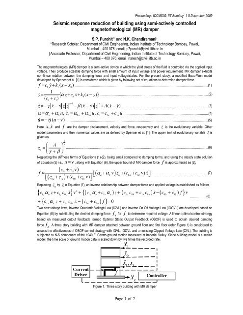
The magnetorhelogical (MR) damper is a semi-active device in which the yield stress of the fluid is controlled via the applied input
voltage. They produce sizeable damping force with small amount of input voltage and power requirement. MR damper exhibits
non-linear relation between the damping force and input voltage/states. For the present study, a modified Bouc-Wen model
developed by Spencer et al. [1] is considered which is given by following set of equations to determine damper force.
…………………………………………………………………………………………………………………..(1)
f = c y&
+ k ( x − x )
1 1 0
y 1
& = { α ( )
0 0 }
( )
z +
c c
c x & + k x −
+
y …………………………………………………………………………………….............(2)
0 1
n−1
n
& & & & & &
z&
=− γ x − y z z −β
( x − y) z + A( x − y)
…………………………………………………………………….........(3)
α = α + α u, c = α + α u,
c = c + c u ………………………………………………………………………...(4)
a b 0 0a 0b 1 1a 1b
u&
=−η
( u − v) …………………………………………………………………………………………………………………………..(5)
Here x,
x& and f are the damper displacement, velocity and force, respectively and z is the evolutionary variable. Other
model parameters and their numerical values are as defined by Spencer et al. [1]. The upper limit of evolutionary variable z is
given as,
1
z
u
⎛ A ⎞
= ⎜
γ + β ⎟
⎝ ⎠
n
……...…………………………………………………………………………………………………………………..(6)
Neglecting the stiffness terms of Equations (1)-(2), being small compared to damping terms, and using the steady state solution
of Equation (5) i.e.,
( c + c v
1a
1b
)
( )
u = v , along with Equation (6), the upper bound of MR damper force f is approximated as [2],
( α α )
& ………………………………………….........(7)
f ≈ ⎡ + v z + ( c + c v) x
a b u 0a 0b
⎤
⎡ c c ( c c v)
⎣
⎦
⎣ + + +
0a 1a 0b 1b
⎤⎦
z by z in Equation (7), an inverse relationship between damper force and applied voltage is established as follows,
Replacing
u
2
{ c1 α
1 0 } v {( ) ( ) ( ) }
b b
z + c c x&
+ c
b b
1a α
b
+ c1b α
a
z + c1 a
c0b + c1b c0 a
x&
− c0b + c1b
f
+ { c α z + c c x&
−
1a 1 0 ( c + c
0 1 ) f } = 0
a a a a a
v
…………….(8)
Two new voltage laws, Inverse Quadratic Voltage Law (IQVL) and Inverse On Off Voltage Law (IOOVL) are developed based on
Equation (8) by substituting the desired damping force
f for f to determine required voltage. A linear optimal control strategy
d
based on measured output feedback termed Optimal Static Output Feedback (OSOF) is used to obtain desired damping
force f . A three story building with MR damper attached between ground floor and first floor (refer Figure 1) is considered to
d
assess the effectiveness of OSOF control strategy with IQVL, IOOVL and an existing Clipped Voltage Law (CVL). The building is
subjected to N-S component of the 1940 El Centro ground motion measured at Imperial Valley. Since building model is a scaled
model, the time scale of ground motion data is scaled down by five times the recorded rate.
Current
Driver
f
x&&
3
x&&
2
x&&
1 , x 1
x&& g
Figure 1. Three story building with MR damper
Controller
Page 1 of 2

Proceedings ICCMS09, IIT Bombay, 1-5 December 2009
The equation of motion for the three story building is given by,
M x&& + C x& + K x = G f − M L && x ……………………………………………………………………………………....(9)
s s s s g
The state space equation representing building dynamics (Equation (9)) and the output equation are,
q&
= A q + B f + E && x g
………………………………………………………………………………………………………………(10)
y = C q + D f ………………………………………………………………………………………………………..........................(11)
The matrix co-efficients of Equation (9) – (10) and their numerical values are as defined by Dyke et al. [3]. The control input (i.e.,
damper force) using OSOF control strategy is given by [4],
f
d
= − K y …………………………………………………………………………………………………………….........................(12)
where, K is the constant feedback gain matrix to be determined. The quadratic Performance Index (PI) defined as,
∞
1 ⎡ T
T ⎤
J = ( f R f ) dt
d d
2 ⎢∫ +
⎣
q Q q ⎥
0
⎦
is used. Here T
Q = C QC ˆ is the positive semi-definite state weighting matrix
with Q ˆ = 1 and R is the positive definite control input weighting matrix. Following Lewis and Syrmos [4], design equations
33
for OSOF control to determine K , which minimizes an optimal cost (i.e., PI) J = 0.5 tr ( PX ) is given as,
T T T
A P + PA + C K RKC + Q =0 …………………………………………………………………………......................(13)
C C
T
A S + SA + X =0 ………………………………………………………………………………………………………………..(14)
C
C
1 1
R − B T PSC T ( CSC T
)
− = K ……………………………………………………………………………………………….....(15)
T
Here, X ≡ q(0) q (0) = I . Coupled nonlinear matrix Equations (13)-(15) are solved by Moerder–Calise iterative algorithm.
To compare the performance of OSOF control strategy, an existing control like Passive On and LQG with COC voltage law are
considered and implemented. The building problem is solved using MATLAB and peak response quantities like interstory drift,
displacement, and acceleration are obtained as shown in Table 1.
Table 1. Peak response quantities of building subjected to El Centro Ground Motion
Control
Strategy
Uncontrolled
Passive On
LQG – COC
(R = 10 -17 )
OSOF – COC
(R = 10 -17 )
OSOF – IQVL
(R = 10 -06 )
OSOF – IOOVL
(R = 10 -08 )
Displacement
(cm)
Interstory
Drift (cm)
Acceleration
(cm/sec 2 )
0.547 0.547 873.69
0.835 0.318 1069.4
0.971 0.202 1408
0.079 0.079 273.96
0.1952 0.157 495.96
0.3044 0.11 767.15
0.1204 0.1204 757.4
0.1876 0.098 733.08
0.2177 0.106 735.37
0.1203 0.1203 711.19
0.1739 0.100 383.19
0.2392 0.0796 553.86
0.1274 0.1274 717.68
0.1883 0.115 468.98
0.2532 0.0806 561.17
0.1149 0.1149 783.01
0.1578 0.1033 438.1
0.2277 0.0797 554.58
MR Damper
Force (N)
Performance
Index
- -
964.69 -
969.72 7.007
809.21 5.2378
768.5 5.589
905.79 5.5149
It is concluded from the present study that OSOF control works well with MR damper. A reduction in maximum peak interstory
drift and PI is obtained when using OSOF control as compared to passive-on/LQG – CVL control. The peak values of
accelerations are also reduced via OSOF control, except when considering first storey accelerations using passive-on control.
References
1. Spencer BF Jr., Dyke SJ, Sain MK, Carlson JD, 1996, Phenomenological model of a magnetorhelogical damper, ASCE
Journal of Engineering Mechanics, 123(3), 230-238.
2. Change Chih-chen, Zhou Li, 2002, Neural network emulation of inverse dynamics for a magnetorhelogical damper, ASCE
Journal of Engineering Mechanics, 128(2), 231-239.
3. Dyke SJ, Spencer BF Jr., Sain MK, Carlson JD, 1996, Seismic response reduction using mangetorhelogical dampers,
Proceedings of IFAC World Congress, San Franscisco, California, June 30 – July 5.
4. Lewis FL, Syrmos VL, 1995, Optimal Control, John Wiley & Sons, Inc., New York, 359-370.
Page 2 of 2