Canadian Meteor Orbit Radar (CMOR) - Meteor Physics Group

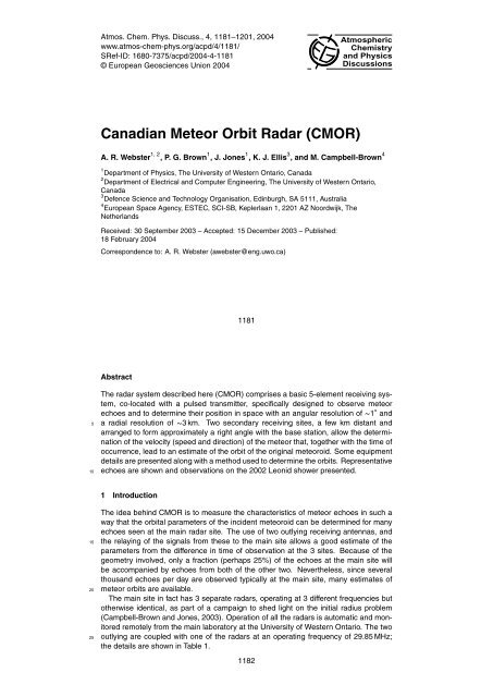
Atmos. Chem. Phys. Discuss., 4, 1181–1201, 2004
www.atmos-chem-phys.org/acpd/4/1181/
SRef-ID: 1680-7375/acpd/2004-4-1181
© European Geosciences Union 2004
Atmospheric
Chemistry
and Physics
Discussions
Canadian Meteor Orbit Radar (CMOR)
A. R. Webster 1, 2 , P. G. Brown 1 , J. Jones 1 , K. J. Ellis 3 , and M. Campbell-Brown 4
1 Department of Physics, The University of Western Ontario, Canada
2 Department of Electrical and Computer Engineering, The University of Western Ontario,
Canada
3 Defence Science and Technology Organisation, Edinburgh, SA 5111, Australia
4 European Space Agency, ESTEC, SCI-SB, Keplerlaan 1, 2201 AZ Noordwijk, The
Netherlands
Received: 30 September 2003 – Accepted: 15 December 2003 – Published:
18 February 2004
Correspondence to: A. R. Webster (awebster@eng.uwo.ca)
1181
Abstract
5
10
The radar system described here (CMOR) comprises a basic 5-element receiving system,
co-located with a pulsed transmitter, specifically designed to observe meteor
echoes and to determine their position in space with an angular resolution of ∼1 ◦ and
a radial resolution of ∼3 km. Two secondary receiving sites, a few km distant and
arranged to form approximately a right angle with the base station, allow the determination
of the velocity (speed and direction) of the meteor that, together with the time of
occurrence, lead to an estimate of the orbit of the original meteoroid. Some equipment
details are presented along with a method used to determine the orbits. Representative
echoes are shown and observations on the 2002 Leonid shower presented.
1 Introduction
15
20
25
The idea behind CMOR is to measure the characteristics of meteor echoes in such a
way that the orbital parameters of the incident meteoroid can be determined for many
echoes seen at the main radar site. The use of two outlying receiving antennas, and
the relaying of the signals from these to the main site allows a good estimate of the
parameters from the difference in time of observation at the 3 sites. Because of the
geometry involved, only a fraction (perhaps 25%) of the echoes at the main site will
be accompanied by echoes from both of the other two. Nevertheless, since several
thousand echoes per day are observed typically at the main site, many estimates of
meteor orbits are available.
The main site in fact has 3 separate radars, operating at 3 different frequencies but
otherwise identical, as part of a campaign to shed light on the initial radius problem
(Campbell-Brown and Jones, 2003). Operation of all the radars is automatic and monitored
remotely from the main laboratory at the University of Western Ontario. The two
outlying are coupled with one of the radars at an operating frequency of 29.85 MHz;
the details are shown in Table 1.
1182

2 The equipment
2.1 The main system
5
10
15
20
The transmitter is located at the main site and the receiving system consists of 5
spaced antennas arranged as two three-element arrays along orthogonal axes with
the center antenna common to both (Fig. 1). The key point of this arrangement is that
the separation between the center antenna and the two outer antennas in each array
differ by one half-wavelength (λ/2). This allows an accurate unambiguous estimate of
the angle-of-arrival (ξ) relative to the array axis (Fig. 2) from the two estimates in Eq.(1),
the first giving an accurate but multi-valued estimate and the second an unambiguous,
less accurate, value which allows selection of the correct estimate.
sin ξ = − λ (φ 10 − φ 20 )
= − λ
2π (d 1 + d 2 ) 2π
(φ 10 + φ 20 )
. (1)
(d 1 − d 2 )
Conversion to elevation and azimuthal angles is straightforward and the array dimensions
used lead to an accuracy of ±1.0 ◦ for elevation angles above 30 ◦ and signal:noise
greater than 10 dB; the principle is discussed in more detail by Jones et al. (1998.) The
antennas are arranged at a height above ground that gives all-round coverage. Echoes
from the main system for 19 November 2002 are shown in Fig. 3 in which the “deadtime”
from the pulse repetition frequency used is clearly visible and the distribution is
entirely consistent with the antenna radiation pattern and the general radiant distribution.
2.2 The outlying receivers
In order to determine the orbit of individual meteoroids, additional information is needed
over and above the accurate position in space of the resultant meteor. One approach
is to establish two extra remote receiving sites and determine the time of observation
of some characteristic part of the meteor echo at each of the three sites as proposed
1183
5
10
by T. R. Kaiser (Hawkins, 1964). As a compromise between high rate of simultaneous
observation and high accuracy in the final answer, which are to some extent in conflict,
a right-angle arrangement with separation of ∼8 km is generally taken as optimum.
Practical considerations regarding site location do come into play and the values used
here are shown in Fig. 4, and are close to the optimum.
Antennas identical to those at the receiving site were used at the remote sites. The
output at 29.85 MHz was translated up to 435 MHz and transmitted to the main site
where it was heterodyned back down to the lower frequency and inserted into the main
receiver; the receiver was designed with 7 separate channels. Software routines in the
main system compare the echoes and their timing to allow determination of the orbit in
cases where echoes are received at all three locations.
3 Derivation of orbital parameters
15
20
25
In order to arrive at an estimate of the orbital parameters of the meteoroid in space
before it interacts with the Earth, the orientation and speed of the observed meteor
need to be determined. Additionally, corrections for the influence of the Earth, its orbital
and rotational speeds and the effects of its gravity and atmosphere (in decelerating the
meteoroid) need to be made in the final estimate; the first three are straightforward but
the last one is more contentious and needs some care; further work on this aspect is
desirable.
The basic idea behind the approach is illustrated in Fig. 5. The direction from the
main site to the meteor, unit vector d, is known from the array measurements and this
is perpendicular to the meteor train. The unit vector p is perpendicular to the vertical
plane containing the meteor so that the direction of the meteor, u, is simply given by
the dot product of d and p, i.e. u=d.p, which establishes the direction. What now
remains is to determine the orientation of the vertical plane, i.e. the angle Ψ.
Figure 6 shows a plan view of the situation in Fig. 5 with the 3-station arrangement
relative to some arbitrary direction, x say. The time of observation of some characteris-
1184

tic point on the train, say the point of maximum increase in amplitude of the echo, leads
to times t 1 , t 2 and t m for the three stations. Labelling T 1 = t 1 −t m and T 2 = t 2 −t m , the
required angle, Ψ, is given by,
5
10
15
20
tan ψ = T 2 x 1 −T 1 x 2
T 1 y 2 −T 2 y 1
, (2)
where the coordinates represent the positions of the two outer stations relative to the
main station. The direction of the (horizontal) unit vector, p, is now known so that the
meteor direction, u, is given by
u = d x p = u x i + u y j + u z k, (3)
and the speed, v, by
v = u x. (x 1 y 2 − x 2 y 1 )
2. (T 1 y 2 − T 2 y 1 )
= u y . (x 1 y 2 − x 2 y 1)
2. (T 1 x 2 − T 2 x 1 ) . (4)
Depending on the orientation of the meteor, the appropriate version of Eq. (4) is used.
Alternative approaches for the determination of the speed from the data available
from the 5 channels of the main receiver are possible. As the meteor echo develops,
the rising amplitude gives estimates from (i) the phase of the echo prior to the point of
orthogonality (the pre-t o approach), or (ii) the amplitude oscillations after this point as
successive Fresnel zones are uncovered, or (iii) the rise-time itself. The last approach
has proved to be most tractable and is illustrated in Fig. 7 in which the distance, x, is
expressed in units of the first Fresnel zone relative to the specular point, i.e. distance
in km, s = F 1 . . x/ √ 2. The speed, v, can be estimated from the maximum slope and the
maximum amplitude of the echo (Baggaley et al, 1997), i.e.
v = ds 1.657.prf. (Rλ)1/2
=
dt 2A max
( dA
dn
)
max
, (5)
where n is the sample number arising from the pulse repetition frequency (prf ) at 1
sample/pulse, (dA/dn) max is the maximum slope, R is the range in km and A max is the
1185
5
peak amplitude of the echo. The value of A max sometimes can be hard to estimate if the
echo is persistent and the train is distorted resulting in increased amplitude after the
echo is established, especially if automatic computer routines are used. An alternative
is to use the amplitude A m at the point of maximum slope so that
1.212.prf. (Rλ)1/2
v =
2A m
( ) dA
. (6)
dn max
4 Experimental results
10
15
20
25
An example of a meteor observed at all 3 stations is shown in Fig. 8; application of
Eqs. (4) and (6) gives respective estimates of the speed, v, of 57.9 and 61.9 km s −1 .
In these estimates, the maximum slope position and value were estimated by fitting a
parabola to the 3 adjacent points around the peak. Another approach is to determine
the position of the centroid of the points around the peak, which gives comparable
answers and has been used extensively in the automated software.
Estimated orbital parameters are generated automatically and here we examine data
taken on 19 November 2002 during the Leonid shower. The time interval used was
00:00 to 24:00 UT and the observed peak in activity was about 1 h in extent centered
at about 10:40 UT. The total number of echoes observed during this 24-h period was
8435 as shown in Fig. 3 above. Of these, 2128 echoes were captured also on both of
the outlying stations allowing an estimate of the speed and orbital parameters.
A plot of the radiant position for each of the above 2128 echoes is shown in Fig. 9.
The clustering of echoes around the nominal Leonid radiant (declination 22 ◦ , right ascension
152 ◦ ) is apparent. A second more diffuse clustering is consistent with the expected
Taurid radiant, which is active for most of November. Selecting meteors that are
within ±5 ◦ of the nominal Leonid radiant results in 165 such echoes. The distribution in
speed for these 165 echoes is shown in Fig. 10, giving an estimate of 69.8±0.8 km s −1 ,
consistent with the accepted value; the distribution of speeds for all echoes on that day
1186

5
are also shown for comparison.
Distributions of orbital inclination (i), perihelion distance (q) and argument of perihelion
(ω) are shown in Fig. 11 for the 165 “Leonid” meteors along with the nominal
values (see McKinley, 1961). The agreement is apparent.
The distribution of speeds for the 2128 3-station meteors as a function of the Right
Ascension (R.A.) is shown in Fig. 12, where the clustering associated with the Leonids
and Taurids is again apparent.
5 Discussion
10
15
20
In determining the orbital elements of individual meteoroids from the 3-station measurements,
it is clear that a good estimate of some of the elements is provided. Others
though, notably the eccentricity (e) and the semi-major axis (a), are very dependent
on the estimate of the speed of the meteor. The fairly wide spread (standard deviation
∼10 km s −1 )in the speed distribution of the meteors within 5 ◦ of the Leonid radiant may
be partly due to the fact that a few non-Leonids will be included, but mostly due to the
inherent uncertainty in the estimate. This is further illustrated by the relatively large
number of apparently hyperbolic meteors (v>72 km s −1 ), shower and sporadic alike, in
Fig. 12, which is not interpreted as a true representation.
Nevertheless, the results are encouraging and techniques for improving the estimates
of the various quantities, especially the speed, are being pursued. These include
improved signal processing and estimation of the time difference between the
echoes at the 3 stations.
Acknowledgements. The authors would like to acknowledge the invaluable assistance of
Z. Krzeminski and R. Weryk.
1187
References
5
10
Baggaley, W. J., Bennett, R. G. T., and Taylor, A. D.: Radar meteor atmospheric speeds determined
from echo profile measurements, Planet. Space Sci., 45, 5, 577–583, 1997.
Campbell-Brown, M. and Jones, J.: Determining the initial radius of meteor trains: fragmentation,
Monthly Notice of the Royal Astronomical Society, 343, 3, 2003.
McKinley, D. W. R.: Meteor Science and Engineering, McGraw-Hill, 1961.
Hawkins, G. S.: Meteors, Comets and Meteorites, McGraw-Hill, 44, 1964.
Jones, J., Webster, A. R., and Hocking, W. K.: An improved interferometer design for use with
meteor radars, Radio Sci., 33, 1, 55–65, 1998.
1188

Table 1. The radar details.
Frequency 29.85 MHz
Peak power 6 kW
P.R.F.
532 pps
Sampling rate 50 ksps
Range increment 12 km
Bandwidth 25 kHz
Pulse length 75 µs
Magnitude limit +6.8
1189
2.5λ
2.5λ
2.0λ
2.0λ
Fig. 1. The layout of the main site receiving antenna system consisting of two orthogonal
Fig. 1 The layout of the main site receiving antenna system consisting of two orthogonal
three-element arrays
three-element
of vertically
arrays of
pointing
vertically
Yagi
pointing
antennas.
Yagi antennas.
1190

ξ
d 1 d 2
1 0 2
Fig. 2. The 3-element array used to determine the angle-of-arrival, ξ; the separations used are
Fig. 2 The 3-element d 1 = 2.0λ andarray d 2 = 2.5λ. used to determine the angle-of-arrival, ξ ; the separations
used are d 1 = 2.0 λ and d 2 = 2.5 λ
1191
19 Nov 2002, 24 hours UT
8435 meteors
Horizontal distance from main site
90
400
120
60
300
N
150
200
30
100
400
180
300
200
100
0
0
0
0
0 100 200 300 400
100
210
200
330
300
240
400
270
300
Fig. 3. Fig.3 The distribution The of echoes of on on the 100km surface. The The distribution consistent
consistent with
the antenna radiation with the antenna patterns radiation and the patterns overall and radiant the overall distribution. radiant distribution. Note theNote sharp the boundary
of the blankingsharp period boundary associated of the blanking with the period “next associated transmitted with pulse” the “next which transmitted is consistent with the
accuracy (±1.0 pulse” ◦ ) in AOA which quoted. is consistent with the accuracy (±1.0 0 ) in AOA quoted.
1192

Thames Bend
2
8.06km
1
Gerber
N
96.8 0 6.16km
m
Main site
Fig. 4. The geographical layout of the 3-station system showing the main site, m, and the two
outlying sites, 1 and 2.
Fig.4 The geographical layout of the 3-station system showing the main site, m, and the
two outlying sites, 1 and 2.
1193
d
p
u
m
x
Ψ
Fig. 5. Determination of the meteor direction vector u from the unit vector d from the main
station and the unit vector p perpendicular to the vertical plane containing the meteor; this
plane is oriented at an angle ψ to a horizontal reference direction x.
Fig.5 Determination of the meteor direction vector u from the unit vector d from
the main station and the unit vector 1194 p perpendicular to the vertical plane
containing the meteor; this plane is oriented at an angle ψ to a horizontal
reference direction x.

m
2
v
y
ψ
x
1
Fig. 6. A plan view of the meteor trail showing the specular reflection points from the transmitter
to the 3 receiving sites m, 1 and 2 (refer to Fig. 4).
Fig. 6 A plan view of the meteor trail showing the specular reflection points from the
transmitter to the 3 receiving sites m, 1 and 2 (refer to fig.4).
1195
1.5
Normalised Meteor Echo
A max = 1.171
Amplitude and Slope
1.0
0.5
A m = 0.854
(dA/dx) max
= 0.707
0.0
-3 -2 -1 0 1 2 3
x
Fig. 7. Showing the classic rise in amplitude of a meteor echo on a back-scatter radar (heavy
Fig. 7 line) Showing and the slope the classic of the amplitude rise in amplitude (light line). The of a abscissa meteor isecho in terms on a ofback-scatter x, related to the radar
physical (heavy distance line) sand along the theslope trail byof s = the F 1 .x/ amplitude √ 2, where (light F 1 is theline). magnitude The of abscissa the first Fresnel is in terms of
zone about the specular point.
x, related to the physical distance
1196
s along the trail by s = F 1 .x/√2, where F 1 is the
magnitude of the first Fresnel zone about the specular point.

Amplitude
55000
50000
45000
40000
35000
30000
25000
20000
MW20011005.000B3
Rnge Hght Theta Phi Amp PRF
122.0 99.8 35.4 150.7 18513.0 532
m
400 450 500 550 600
30000
1
2
Amplitude differential
20000
10000
0
-10000
400 450 500 550 600
Sample Number
Fig. 8. A meteor echo observed on all three stations showing the amplitudes (offset for clarity)
and derived Fig.8 slope. A The meteor timecho delays observed result on in all an three estimate stations showing of v = 57.9 the amplitudes km s −1 , while (A/D output the rise-time
gives a value of 61.9 value kmand s −1 offset . for clarity) and derived slope. The time delays result in an
estimate of v = 57.9km.s -1 , while the rise-time gives a value of 61.9km.s -1 ; m is
the main station.
1197
80
60
021119 UT 24 hours
Declination, deg.
40
20
0
-20
-40
-60
-80
Taurids
apex
Leonids
anti-apex
0 60 120 180 240 300 360
RA, deg.
Fig. 9. The celestial coordinates of the radiants of the 2128 meteors observed by all 3 stations.
The clustering around the expected value for the Leonids is apparent, as is the more diffuse
radiant structure of the Taurids. The general sporadic background is a maximum in the direction
Fig. of the 9 The Earth’s celestial way (thecoordinates apex) and a minimum of the radiants towards of the the anti-apex. 2128 meteors Radiants observed below −47 ◦ by in all 3
declination stations. are not The visible clustering from this around location. the expected value for the Leonids is apparent, as
is the more diffuse radiant structure of the Taurids. The general sporadic
background is a maximum in the direction of the Earth’s way (the apex) and a
minimum towards the anti-apex. 1198 Radiants below –47 0 in declination are not
visible from this location.

250
200
All echoes
(2128)
Number
150
100
50
Number
0
40
30
20
10
0 10 20 30 40 50 60 70 80 90 100
Echoes with radiant within
5 0 of dec = +22 0 , RA = 152 0
Speed, km.s -1
Mean 68.7
Std. Dev. 10.2
Std. Err. 0.8
165 echoes
0
0 10 20 30 40 50 60 70 80 90 100
Speed, km.s -1
Fig. Fig. 10. 10. The The distribution distribution of measured if measured speeds speeds for the for 2128 the 2128 echoes echoes observed observed at theat 3the stations 3
and the speed distribution for radiants within 5
stations and the speed distribution ◦ of the expected Leonid radiant.
for radiants within 5 0 of the expected
Leonid radiant.
1199
Number in 2 0 interval
30
25
20
15
10
5
0
0 60 120 180 240 300 360
Orbit Inclination, i, deg.
Number in 0.02 interval
80
60
40
20
0
0.0 0.5 1.0
Perihelion, q, a.u.
Number in 5 0 interval
40
30
20
10
0
0 60 120 180 240 300 360
Argument of perihelion, ω, deg.
Fig. 11. Selected Fig. 11 orbital Selected elements orbital elements for the for 165 the 165 echoes echoes with with radiants radiants within within 5 0 of 5 ◦ the of the expected
value.
expected value. The nominal values are as indicated.
1200

Speed, km.s -1
100
90
80
70
60
50
40
30
20
10
0
0 90 180 270 360
R.A.
Apex
Anti-apex
Fig. 12. The distribution in speed versus R.A. for the 2128 echoes seen on all 3 stations. The
Fig. Leonid 12 The andistribution Taurid radiant in again speed areversus apparent, R.A. as isfor the the expected 2128 generally echoes seen increased on all speed 3 stations. in
the direction The Leonid of the apex. and Taurid radiant again are apparent, as is the expected increased
speed in the direction of the apex.
1201